Generalized Rational Multi-step Method for Delay Differential Equations

Generalized Rational Multi-step Method for Delay

Differential Equations

1

_{J. Vinci Shaalini,}

_{A. Emimal Kanaga Pushpam}

Abstract- This paper presents the generalized rational multi-step method for solving delay differential equations (DDEs). Here, we develop the r-step p-th order generalized multi-step method which is based on rational function approximation technique. The local truncation error and stability analysis are given. The delay argument is approximated using Lagrange interpolation. The applicability of this method has been demonstrated by numerical examples of DDEs with constant delay (HIV-1 infection model), time dependent delay and state dependent delays.

Index Terms-Lagrange interpolation, Multi-step Method, Rational function, Stability polynomial and Stability region, Delay differential equations, HIV-1 infection model.

I. INTRODUCTION

Delay differential equations (DDEs) are a type of differential equations in which the derivative of the unknown function depends not only at its present time but also at the previous times. In ordinary differential equations (ODEs), a simple initial condition is given. But to specify DDEs, additional information is needed. Because the derivative depends on the solution at the previous times, an initial history function which gives information about the solution in the past needs to be specified. A general form of the first order DDE is

𝑦′(𝑡) = 𝑓(𝑡, 𝑦(𝑡), 𝑦(𝑡 − 𝜏)), 𝑡 > 𝑡0

𝑦(𝑡) = Φ(𝑡), 𝑡 ≤ 𝑡0 (1)

where Φ(t) is the initial function and τ is the delay term. The function Φ(t) is known as the ‘history function’, as it gives information about the solution in the past. If the delay term τ is a constant, then it is called constant delay. If it is function of time t, then it is called time dependent delay. If it is a function of time t and y(t), then it is called state dependent delay.

These equations arise in population dynamics [1], control systems [2], chemical kinetics [3], and in several areas of science and engineering. Recently there has been a growing interest in obtaining the numerical solutions of stiff and non-stiff DDEs. Rostann [4] et al. implemented Adomian Decomposition Method for solving system of DDEs. Radzi [5] et al. developed the two and three point one-step block method for solving DDEs. Fuziyah Ishak et al. [6] described block method for solving Pantograph type functional DDEs. Toheeb et al. [7] obtained the exact/approximate solution of DDEs by using the combination of Laplace and the variational iteration

Manuscript received May 6, 2019; revised September 19, 2019.

1_{J. Vinci Shaalini is with the Mathematics Department, Bishop Heber}

College, Tiruchirappalli 620017, Tamilnadu, India. (e-mail: [email protected]).

2*_{A. Emimal Kanaga Pushpam is with the Mathematics Department,}

Bishop Heber College, Tiruchirappalli 620017, Tamilnadu, India. (e-mail: [email protected]).

method. Emimal and Vinci [8] proposed RK method based on Harmonic Mean for solving DDEs with constant lags.

Several numerical methods have been constructed for solving stiff DDEs. Bocharov [9] applied linear multi-step methods for the numerical solution of stiff delay differential systems modelling an immune response. Vinci and Emimal [10, 11] proposed composite RK methods and a new one step method based on polynomial scheme for solving stiff and non-stiff DDEs.

Several multi-step techniques using variety of interpolating polynomials and functions have been developed to solve ODEs. Simon Ola Fatunla [12] developed the nonlinear multistep methods based on inverse polynomial for solving IVPs. Okosun and Ademiluyi [13] derived two-step second order inverse polynomial methods for integration of differential equations with singularities. Abolarin and Akingbade [14] derived the fourth stage inverse polynomial scheme IVPs. Teh Yuan Ying et al. [15] proposed a new class of rational multi-step methods for solving IVPs.

In this paper we present the r-step p-th order generalized rational multi-step method for solving DDEs which is based on rational function approximation technique. This method has been referred here as GRMM (r, p). The organization of this paper is as follows:

In section II, the derivation of GRMM (r, p) is given. In section III, the implementation of GRMM for 2-step and of orders 2, 3 and 4 is presented. In section IV, the stability analysis of GRMM (2, p), (p = 2, 3, 4) has been given. In section V, numerical illustrations of DDEs are provided to demonstrate the efficiency of this method.

II. DERIVATION OF GENERALISED RATIONAL MULTI-STEP METHOD (GRMM (r, p))

Assume that the analytical solution 𝑦𝑛+𝑟 = 𝑦(𝑡𝑛+𝑟) to the initial value problem (1) can be given by

𝑦𝑛+𝑟 = 𝑎0+ 𝑎1ℎ 1+∑𝐾𝑗=1𝑏𝑗ℎ𝑗

, 1 + ∑𝐾𝑗=1𝑏𝑗ℎ𝑗≠ 0 (2)

where 𝑎0, 𝑎1, 𝑏𝑗,(j = 1,2,…K) are coefficients that need to be

determined.

With the GRMM (r, p) in (2), we associate the difference operator L defined by

𝐿[𝑦(𝑡); ℎ]𝐺𝑅𝑀𝑀(𝑟,𝑝)= (𝑦(𝑡 + 𝑟ℎ) − 𝑎0) × (1 + ∑𝐾𝑗=1𝑏𝑗ℎ𝑗) − 𝑎1ℎ

(3)

where y(t) is an arbitrary, continuous and differentiable function.

IAENG International Journal of Applied Mathematics, 50:1, IJAM_50_1_13

Expanding 𝑦(𝑡 + 𝑟ℎ) as Taylor series and collecting terms in (3), we have

𝐿[𝑦(𝑡); ℎ]𝐺𝑅𝑀𝑀= 𝐶0ℎ0+ 𝐶1ℎ1+ ⋯ + 𝐶𝐾ℎ𝐾

+𝐶𝐾+1ℎ𝐾+1_{+ ⋯ (4)}

where 𝐶𝑖, 𝑖 = 0,1, … , 𝐾, 𝐾 + 1 are the coefficients that need

to be determined.

Taking K=p-1 in (2) and expanding 𝑦(𝑡 + 𝑟ℎ) into Taylor series, we get

𝐿[𝑦(𝑡); ℎ]𝐺𝑅𝑀𝑀=

−𝑎0+ 𝑦(𝑡) + ℎ(−𝑎1− 𝑎0𝑏1+ 𝑏1𝑦(𝑡) + 𝑟𝑦′(𝑡))

+ℎ2_(−𝑎

0𝑏2+ 𝑏2𝑦(𝑡) + 𝑟 2 2!𝑦

′′_{(𝑡) + 𝑟𝑏}

1𝑦′(𝑡))

+ ⋯

+ℎ𝑝₍𝑟𝑝 𝑝!𝑦

(𝑝)_{(𝑡) +} 𝑟𝑝−1 (𝑝−1)!𝑏1𝑦

(𝑝−1)_{(𝑡) + ⋯ + 𝑟𝑏}

𝑝−1𝑦′(𝑡))

+ℎ𝑝+1₍𝑟𝑝+1 (𝑝+1)!𝑦

(𝑝+1)_{(𝑡) +} 𝑟𝑝 𝑝!𝑏1𝑦

(𝑝)_{(𝑡) + ⋯ +}

𝑟2 2!𝑏𝑝−1𝑦

′′_(𝑡))

+𝑂(ℎ𝑝+2_{) (5)}

Comparing (4) and (5), we get

𝐶0= −𝑎0+ 𝑦(𝑡),

𝐶1= −𝑎1− 𝑎0𝑏1+ 𝑏1𝑦(𝑡) + 𝑟𝑦′_(𝑡),

𝐶2= 𝑟𝑏1𝑦′(𝑡) + 𝑟2 2!𝑦

′′_{(𝑡) + 𝑏}

2𝑦(𝑡) − 𝑎0𝑏2,

…,

𝐶𝑝=𝑟𝑝 𝑝!𝑦

(𝑝)_{(𝑡) +} 𝑟𝑝−1 (𝑝−1)!𝑏1𝑦

(𝑝−1)_{(𝑡) + ⋯ + 𝑟𝑏𝑝−1𝑦}′_(𝑡),

𝐶𝑝+1=_(𝑝+1)!𝑟𝑝+1 𝑦(𝑝+1)(𝑡) +𝑟𝑝 𝑝!𝑏1𝑦

(𝑝)_{(𝑡) + ⋯ +}

𝑟2 2!𝑏𝑝−1𝑦

′′_(𝑡)

(6)

For p-th order GRMM, we put 𝐶0 =𝐶1 =𝐶2 =…=𝐶𝑝 = 0 in (6)

which gives the following solutions

𝑎0= 𝑦(𝑡),

𝑎1= 𝑟𝑦′(𝑡),

𝑏1= −𝑟𝑦′′(𝑡) 2!𝑦′_(𝑡),

…,

𝑏𝑝−1 = − [ 𝑟𝑝−1

𝑝! 𝑦(𝑝)(𝑡)

𝑦′_(𝑡) +

𝑟𝑝−2 (𝑝−1)!𝑏1

𝑦(𝑝−1)(𝑡) 𝑦′_(𝑡) +

_(𝑝−2)!𝑟𝑝−3 𝑏2𝑦(𝑝−2)(𝑡) 𝑦′_(𝑡) + ⋯ +

𝑟 2!𝑏𝑝−2

𝑦′′(𝑡) 𝑦′_(𝑡)] (7)

and

𝐶𝑝+1=_(𝑝+1)!𝑟𝑝+1 𝑦(𝑝+1)_{(𝑡) +}𝑟𝑝 𝑝!𝑏1𝑦

(𝑝)_{(𝑡) + ⋯ +}

𝑟2 2!𝑏𝑝−1𝑦

′′_(𝑡)

(8)

When 𝑡 = 𝑡𝑛, we can write 𝑦𝑛= 𝑦(𝑡𝑛). Then (7) becomes

𝑎0= 𝑦𝑛,

𝑎1= 𝑟𝑦′ 𝑛,

𝑏1= − 𝑟𝑦′′

𝑛

2!𝑦′ 𝑛

, …,

𝑏𝑝−1 = − [ 𝑟𝑝−1

𝑝! 𝑦_𝑛(𝑝)

𝑦_𝑛′ + 𝑟𝑝−2 (𝑝−1)!𝑏1

𝑦_𝑛(𝑝−1) 𝑦_𝑛′ +

𝑟𝑝−3 (𝑝−2)!𝑏2

𝑦_𝑛(𝑝−2) 𝑦_𝑛′ +

… +𝑟 2!𝑏𝑝−2

𝑦𝑛′′

𝑦_𝑛′] (9)

where 𝑦𝑛= 𝑦(𝑡𝑛) and 𝑦𝑛 (𝑚)

= 𝑦(𝑚)_(𝑡

𝑛), m = 1,2,… by the

localizing assumption. Taking K = p-1 in (2),

𝑦𝑛+𝑟 = 𝑎0+ 𝑎1ℎ

1+𝑏1ℎ+𝑏2ℎ2+⋯+𝑏𝑝−2ℎ𝑝−2+𝑏𝑝−1ℎ𝑝−1,

where 1 + 𝑏1ℎ + 𝑏2ℎ2_{+ ⋯ + 𝑏𝑝−1ℎ}𝑝−1_{≠ 0 (10)}

Substituting (9) in (10),

𝑦𝑛+𝑟 = 𝑦𝑛

+ 𝑟ℎ𝑦𝑛′

1+(−𝑟𝑦𝑛′′

2!𝑦𝑛′)ℎ+

…+(−[𝑟𝑝−1_𝑝! 𝑦𝑛

(𝑝) 𝑦𝑛′ +

𝑟𝑝−2 (𝑝−1)!𝑏1

𝑦𝑛(𝑝−1) 𝑦𝑛′ +

𝑟𝑝−3 (𝑝−2)!𝑏2

𝑦𝑛(𝑝−2) 𝑦𝑛′ +⋯+

𝑟 2!𝑏𝑝−2𝑦𝑛

′′ 𝑦𝑛′])ℎ

𝑝−1

(11)

The local truncation error (LTE) of GRMM (r, p) is given by

𝐿𝑇𝐸𝐺𝑅𝑀𝑀(𝑟,𝑝)= ℎ𝑝+1₍𝑟𝑝+1 (𝑝+1)!𝑦

(𝑝+1)_{(𝑡) +}𝑟𝑝 𝑝!𝑏1𝑦

(𝑝)_{(𝑡) +}

… +𝑟2 2!𝑏𝑝−1𝑦

′′_{(𝑡)) + 𝑂(ℎ}𝑝+2₎

(12)

III. IMPLEMENTATION STRATEGY OF GRMM (r, p)

In this section, GRMM (r, p) is implemented for various steps r and any order p.

For example, here we discuss the implementation of GRMM for 2-step and of orders 2, 3 and 4.

Taking r = 2 and p = 2, 3, 4 in (11) respectively and on simplification, we get

For GRMM (2, 2):

𝑦𝑛+2= 𝑦𝑛+ 2ℎ(𝑦𝑛′)2

𝑦_𝑛′−ℎ𝑦_𝑛′′ (13)

For GRMM (2, 3):

𝑦𝑛+2= 𝑦𝑛+

6ℎ(𝑦_𝑛′)3 3(𝑦_𝑛′₎2_−3ℎ𝑦

𝑛′𝑦𝑛′′+3ℎ2(𝑦𝑛′′)2−2ℎ2𝑦𝑛′𝑦𝑛′′′

(14)

For GRMM (2, 4):

𝑦𝑛+2= 𝑦𝑛+

6ℎ(𝑦𝑛′)4

3(𝑦_𝑛′)3−3ℎ(𝑦_𝑛′)2𝑦_𝑛′′+3ℎ2_𝑦

𝑛′(𝑦𝑛′′)2−3ℎ3(𝑦𝑛′′)3

−2ℎ2(𝑦𝑛′)2𝑦𝑛′′′+4ℎ3𝑦𝑛′𝑦𝑛′′𝑦𝑛′′′−ℎ3(𝑦𝑛′)2𝑦𝑛(4)

(15)

IAENG International Journal of Applied Mathematics, 50:1, IJAM_50_1_13

From (12), the local truncation error of GRMM (2, p), where p = 2, 3, 4 are given respectively by

𝐿𝑇𝐸𝐺𝑅𝑀𝑀(2,2)= ℎ3(− 2(𝑦𝑛′′)2

𝑦_𝑛′ + 4 3𝑦𝑛

′′′_{) + 𝑜(ℎ}4_{) (16)}

𝐿𝑇𝐸𝐺𝑅𝑀𝑀(2,3)= ℎ4( 2(𝑦𝑛′′)3

(𝑦_𝑛′₎2 −

8𝑦𝑛′′𝑦𝑛′′′

3𝑦_𝑛′ +

2 3𝑦𝑛

(4)

) + 𝑜(ℎ5₎

(17)

𝐿𝑇𝐸𝐺𝑅𝑀𝑀3(2,4)=

ℎ5₍−2(9(𝑦𝑛′′)4)−18𝑦𝑛′(𝑦𝑛′′)2𝑦𝑛′′′+4(𝑦𝑛′)2(𝑦𝑛′′′)2+6(𝑦𝑛′)2𝑦𝑛′′𝑦𝑛(4)

9(𝑦_𝑛′₎3 +

4 15𝑦𝑛

(5)

) + 𝑜(ℎ6₎

(18)

In a similar manner, we can implement GRMM (r, p) for various steps r and any order p.

IV. STABILITY ANALYSIS OF GRMM (r, p)

In this section, we derived the stability polynomials of GRMM (2, p), (p = 2, 3, 4) and obtained their corresponding stability regions.

We consider a commonly used linear test equation with a constant delay 𝜏 = 𝑚ℎ where m is a positive integer,

𝑦′_{(𝑡) = 𝜆𝑦(𝑡) + 𝜇𝑦(𝑡 − 𝜏), 𝑡 > 𝑡0}

𝑦(𝑡) = 𝜙(𝑡), 𝑡 ≤ 𝑡0 (19)

where 𝜆, 𝜇 ∈ 𝐶, 𝜏 > 0 and



When p = 2, a slight rearrangement of (13) can be written as

𝑦𝑛+2= 𝑦𝑛+ 2ℎ𝑦𝑛′+ 2ℎ2𝑦𝑛′′ (20)

Using (20) in (19), we get

𝑦𝑛+2= 𝑦𝑛+ 2ℎ(𝜆𝑦𝑛+ 𝜇𝑦(𝑡𝑛− 𝜏))

+2ℎ2_{(𝜆𝑦′𝑛+ 𝜇𝑦′(𝑡𝑛− 𝜏)) (21)}

𝑦(𝑡𝑛− 𝑚ℎ) = 𝑦(𝑡𝑛−𝑚) = ∑𝑠𝑙=−𝑟1 1𝐿𝑙(𝑐𝑖)𝑦𝑛−𝑚+𝑙

with

𝐿𝑙(𝑐𝑖) = ∏

𝑐𝑖−𝑗1

𝑙−𝑗1

𝑠1

𝑗=−𝑟1 , 𝑗1≠ 𝑙 and 𝑟1, 𝑠1> 0

Taking 𝑦(𝑡𝑛− 𝜏) = ∑ 𝐿𝑙(𝑐)𝑦𝑛−𝑚+𝑙 𝑠1

𝑙=−𝑟1 and

𝑦′_(𝑡

𝑛− 𝜏) = 𝜆 ∑𝑠𝑙=−𝑟1 1𝐿𝑙(𝑐)𝑦𝑛−𝑚+𝑙

+𝜇 ∑ 𝐿𝑙(𝑐)𝑦𝑛−2𝑚+𝑙 𝑠₁

𝑙=−𝑟1 (22)

Then (21) becomes

𝑦𝑛+2= 𝑦𝑛+ 2ℎ(𝜆𝑦𝑛+ 𝜇 ∑𝑠𝑙=−𝑟1 1𝐿𝑙(𝑐)𝑦𝑛−𝑚+𝑙)

+2ℎ2₍

𝜆(𝜆𝑦𝑛+ 𝜇 ∑ 𝐿𝑙(𝑐)𝑦𝑛−𝑚+𝑙 𝑠1

𝑙=−𝑟₁ )

+𝜇𝜆 ∑ 𝐿𝑙(𝑐)𝑦𝑛−𝑚+𝑙 𝑠₁

𝑙=−𝑟1

+𝜇 ∑𝑠𝑙=−𝑟1 1𝐿𝑙(𝑐)𝑦𝑛−2𝑚+𝑙 )

𝑦𝑛+2= 𝑦𝑛+ 2𝜆ℎ𝑦𝑛+ 2𝜆2ℎ2𝑦𝑛

+ ∑ 𝐿𝑙(𝑐)𝑦𝑛−𝑚+𝑙 𝑠₁

𝑙=−𝑟1 (2𝜇ℎ + 4ℎ

2_𝜇𝜆)

+ ∑ 𝐿𝑙(𝑐)𝑦𝑛−2𝑚+𝑙 𝑠₁

𝑙=−𝑟1 (2ℎ

2_𝜇2₎

𝑦𝑛+2= 𝑦𝑛(1 + 2𝜆ℎ + 2(𝜆ℎ)2)

+ ∑ 𝐿𝑙(𝑐)𝑦𝑛−𝑚+𝑙 𝑠1

𝑙=−𝑟₁ (𝜇ℎ(2 + 4𝜆ℎ))

+ ∑ 𝐿𝑙(𝑐)𝑦𝑛−2𝑚+𝑙(2(𝜇ℎ)2) 𝑠1

𝑙=−𝑟1

Let 𝛼 = 𝜆ℎ and 𝛽 = 𝜇ℎ then the above equation becomes

𝑦𝑛+2= 𝑦𝑛(1 + 2𝛼 + 2𝛼2)

+(𝛽(2 + 4𝛼)) ∑ 𝐿𝑙(𝑐)𝑦𝑛−𝑚+𝑙 𝑠₁

𝑙=−𝑟1

+2𝛽2_{∑ 𝐿}

𝑙(𝑐)𝑦𝑛−2𝑚+𝑙 𝑠1

𝑙=−𝑟₁

To obtain the stability polynomial, the delay term is approximated using three points Lagrange interpolation.

By putting 𝑛 − 𝑚 + 𝑙 = 0 and 𝑛 − 2𝑚 + 𝑙 = 0 and by taking

l = -1, 0, 1, the stability polynomial will be in the standard form.

The recurrence is stable if the zeros of 𝜁𝑖 of the stability polynomial

𝑆(𝛼, 𝛽: 𝜁) = 𝜁𝑛+2− (1 + 𝛼 + 2𝛼2)𝜁𝑛

−𝛽(2 + 4𝛼)(𝐿−1(𝑐) + 𝐿0(𝑐)𝜁 + 𝐿1(𝑐)𝜁2)

−2𝛽2_(𝐿

−1(𝑐) + 𝐿0(𝑐)𝜁 + 𝐿1(𝑐)𝜁2)

satisfies the root condition|𝜁𝑖| ≤ 1. From this, the stability

polynomial for the method GRMM (2, 2) with 𝜏 = 1 is given as

𝑆(𝛼, 𝛽: 𝜁) = 𝜁𝑛+2_{− (1 + 𝛼 + 2𝛼}2_)𝜁𝑛

−(2𝛽 + 2𝛽2_{+ 4𝛼𝛽)}

Similarly, by considering suitable number of points in Lagrange interpolation according to the order of the method, we can obtain the corresponding stability polynomials of GRMM (2, p).

When p = 3, the stability polynomial for GRMM (2, 3) is given as

𝑆(𝛼, 𝛽: 𝜁) = 𝜁𝑛+2− (1 + 𝛼 + 2𝛼2+4 3𝛼

3_{) 𝜁}𝑛

− (2𝛽 + 2𝛽2+4 3𝛽

3_{+ 4𝛼𝛽 + 4𝛼}2_{𝛽 + 4𝛼𝛽}2₎

When p = 4, the stability polynomial for GRMM (2, 4) is given as

𝑆(𝛼, 𝛽: 𝜁) = 𝜁𝑛+2_{− (1 + 𝛼 + 2𝛼}2₊4 3𝛼

3₊2 3𝛼

4_{) 𝜁}𝑛

− (2𝛽 + 2𝛽2₊4 3𝛽

3₊2 3𝛽

4_{+ 2𝛼𝛽 + 4𝛼}2_{𝛽 +}

4𝛼𝛽2₊8 3𝛼𝛽

3₊8 3𝛼

3_{𝛽 + 4𝛼}2_𝛽2₎

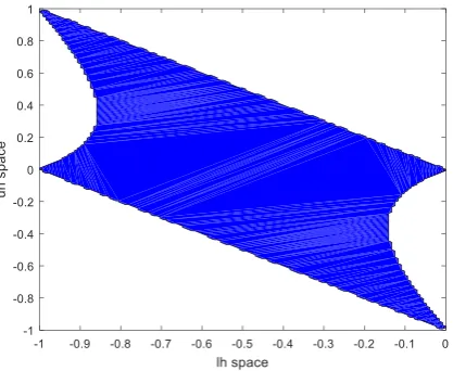
The stability regions of GRMM (2, 2), GRMM (2, 3) and GRMM (2, 4) are given in Fig. 1 -3.

In a similar manner, we can obtain the stability polynomials and their corresponding regions of GRMM with r-step and of any order p.

IAENG International Journal of Applied Mathematics, 50:1, IJAM_50_1_13

V. NUMERICAL EXAMPLES

Example 1:

Consider the stiff linear system of DDEs with multiple delays

𝑦1′(𝑡) = − 1 2𝑦1(𝑡) −

1

2𝑦2(𝑡 − 1) + 𝑓1(𝑡),

𝑦2′_{(𝑡) = −𝑦} 2(𝑡) −

1

2𝑦1(𝑡 − 1

2) + 𝑓2(𝑡), 0 ≤ 𝑡 ≤ 1

with initial conditions

𝑦1(𝑡) = 𝑒−𝑡/2, −1

2 ≤ 𝑡 ≤ 0,

𝑦2(𝑡) = 𝑒−𝑡, − 1 ≤ 𝑡 ≤ 0

and 𝑓1(𝑡) = 1 2𝑒

−(𝑡−1)_{, 𝑓} 2(𝑡) =

1 2𝑒

−(𝑡−1/2)/2

The exact solution is

𝑦1(𝑡) = 𝑒−𝑡/2_{, 𝑦2(𝑡) = 𝑒}−𝑡

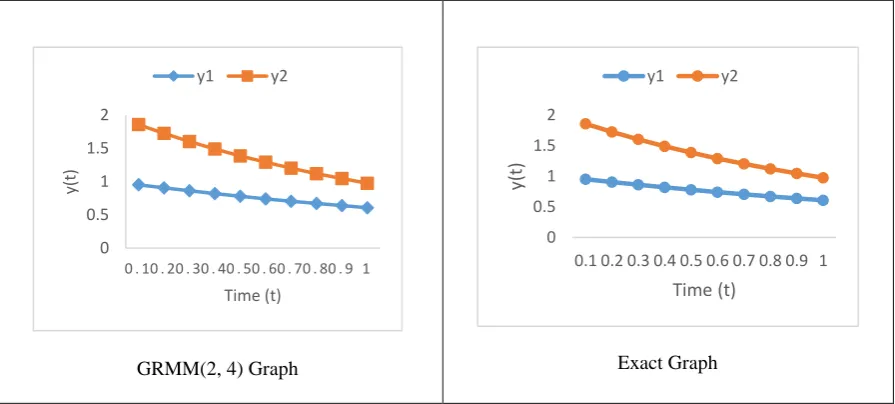
By taking h = 0.01 in the above examples, the absolute errors of GRMM (2, p) where p = 2, 3, 4 are given in Tables 1 – 2 and the graphs are shown in Fig. 4.

Example 2:

Consider the time dependent DDE

𝑦′_{(𝑡) =}𝑡−1

𝑡 𝑦(ln(𝑡) − 1)𝑦(𝑡), 𝑡 ≥ 1

with initial condition

𝑦(𝑡) = 1, 𝑡 ≤ 1

and the exact solution is

𝑦(𝑡) = exp (𝑡 − ln(𝑡) − 1), 𝑡 ≥ 1

By taking h = 0.01 in the above examples, the absolute errors of GRMM (2, p) where p = 2, 3, 4 are given in Table 3 and the graphs are shown in Fig. 5.

Example 3:

Consider the state dependent DDE

𝑦′_{(𝑡) = cos (𝑡)𝑦(y(t) − 2), 𝑡 ≥ 0}

with initial condition

𝑦(𝑡) = 1, 𝑡 ≤ 0

and the exact solution is

𝑦(𝑡) = sin(𝑡) + 1, 0 ≤ 𝑡 ≤ 1

By taking h = 0.01 in the above examples, the absolute errors of GRMM (2, p) where p = 2, 3, 4 are given in Table 4 and the graphs are shown in Fig. 6.

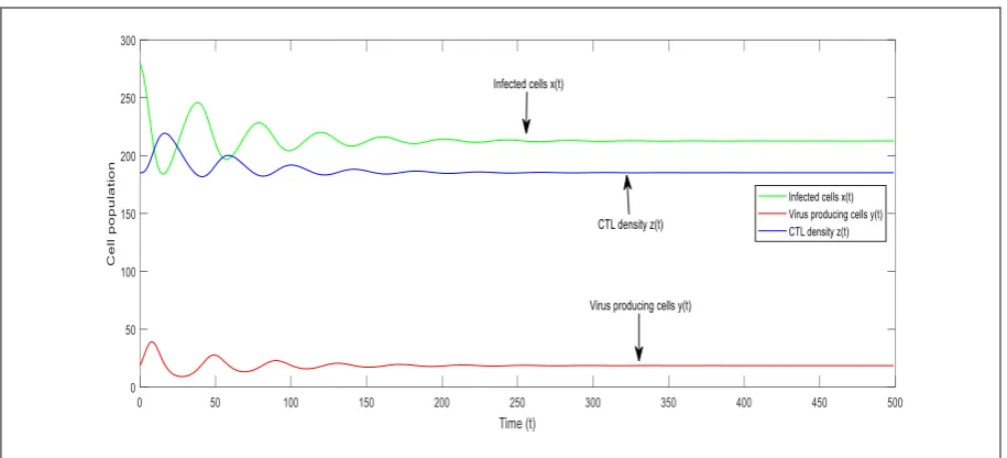
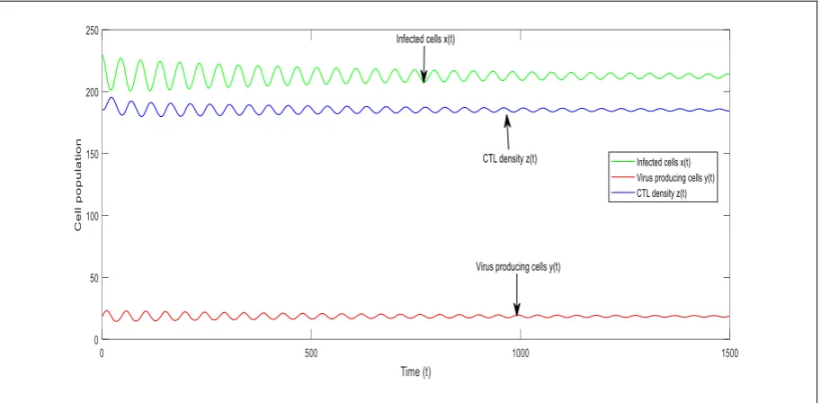
Example 4: (HIV-1 infection model)

Consider a mathematical model of HIV-1 infection to CD4+ T cells including the inhibitor drug discussed in [16]. Let x(t) be the number of infected cells and y(t) be the number of virus producing cells and z(t) be the density of the Cytotoxic T-Lymphocyte (CTL) responses against virus-infected cells.

Model 1:

In this basic delay HIV-1 infection model, we assume that the virus producing cells are killed by CTL instantaneously. When the delay 𝜏 is small, this model can be represented by the following set of equations

𝑑𝑥

𝑑𝑡= 𝜆 − 𝑑𝑥 − 𝛽𝑥(𝑡 − 𝜏)𝑦(𝑡 − 𝜏)

𝑑𝑦

𝑑𝑡 = 𝛽𝑥(𝑡 − 𝜏)𝑦(𝑡 − 𝜏) − 𝑎𝑦 − 𝑝𝑦𝑧

𝑑𝑧

𝑑𝑡 = 𝑘𝑦 − 𝑏𝑧

Model 2:

In reality, there is a latency period during the process of killing of virus-producing cells by CTL. (i.e. not instantaneous as in Model 1). Hence we include a delay in the terms representing killing of virus-producing cells by CTL and in the stimulation of CTL. The model equations are given by

𝑑𝑥

𝑑𝑡= 𝜆 − 𝑑𝑥 − 𝛽𝑥𝑦

𝑑𝑦

𝑑𝑡 = 𝛽𝑥𝑦 − 𝑎𝑦 − 𝑝𝑦(𝑡 − 𝜏)𝑧

𝑑𝑧

𝑑𝑡= 𝑘𝑦(𝑡 − 𝜏) − 𝑏𝑧

Model 3:

In this model, we include the delays exist in the process of infection of healthy T cells and also in the terms representing killing of virus-producing cells by CTL and in the stimulation of CTL together. The model equations can be represented by the following set of equations

𝑑𝑥

𝑑𝑡= 𝜆 − 𝑑𝑥 − 𝛽𝑥(𝑡 − 𝜏1)𝑦(𝑡 − 𝜏1)

𝑑𝑦_𝑑𝑡 = 𝛽𝑥(𝑡 − 𝜏1)𝑦(𝑡 − 𝜏1) − 𝑎𝑦 − 𝑝𝑦(𝑡 − 𝜏2)𝑧

𝑑𝑧_𝑑𝑡= 𝑘𝑦(𝑡 − 𝜏2) − 𝑏𝑧

The variables and parameters used in these three models are given in Table 5.

For the Models 1 and 2, the initial conditions are taken as x(θ) = 280.0, y(θ) = 18.5189 and z(θ) = 185.1893 and for the Model 3 as

x(θ) = 230.0, y(θ) = 18.5189 and z(θ) = 185.1893 where θ∈(-τ,0].

The numerical simulations of these models by GRMM (2, 4) are given in Fig. 7 - 9.

IAENG International Journal of Applied Mathematics, 50:1, IJAM_50_1_13

VI. CONCLUSION

In this paper, the generalized rational multi-step method of r-step and p-th order by means of rational interpolating function is presented for solving DDEs. The local truncation errors have been determined. The stability polynomials of GRMM (2, p) where p = 2, 3, 4 are derived and their corresponding stability regions are obtained. The delay argument is approximated using Lagrange interpolation.

Numerical examples of DDEs with constant delay, time dependent delay and state dependent delays have been considered to demonstrate the efficiency of the proposed method. From the Tables 1 – 4, it is evident that the proposed method gives results with good accuracy. In HIV-1 infection model, the solution graphs are well comparable with the numerical simulations given in [16]. Hence, it is concluded that the proposed GRMM (r, p) is suitable for solving DDEs.

REFERENCES

[1] Y. Kuang, “Delay differential equations with applications in population dynamics,” Academic Press, Boston, San Diego, New York, 1993.

[2] E. Fridman, L. Fridman, E. Shusti, “Steady modes in relay control systems with time delay and periodic disturbances,” Journal of Dynamical Systems Measurement and Control, vol. 122, no. 4, pp. 732-737, 2000.

[3] I. Epstein, Y. Luo, “Differential delay equations in chemical kinetics: non-linear models; the cross-shaped phase diagram and the oregonator,” Journal of Chemical Physic., vol.95, no. 1, pp. 244-254, 1991.

[4] Rostann K. Saeed, Botan M. Rahman, “Adomian decomposition method for solving system of delay differential equation,” Australian Journal of Basic and Applied Sciences, vol. 4, no. 8, pp. 3613-3621, 2010.

[5] H.M. Radzi, Zanariah Abdul Majid, Fudziah Ismail, Mohamed Suleiman, “Two and three point one-step block method for solving delay differential equations,” Journal of Quality Measurement and Analysis,

vol.8, no. 1, pp. 29-41, 2012.

[6] Fuziyah Ishak, Mohamed B. Suleiman, Zanariah A. Majid, “Block Method for solving Pantograph-type functional differential equations,”

Proceeding of the World Congress on Engineering, vol. 2, 2013.

[7] Toheeb A. Biala, Oladapo O. Asim, Yusuf O. Afolabi, “A combination of the Laplace and the variational iteration method for the analytical treatment of delay differential equations,” International Journal of Differential Equations and Applications, vol.13, no. 3, pp. 164-175,

2014.

[8] A. Emimal Kanaga Puhpam, J. Vinci Shaalini, “Solving delay differential equations with constant lags using RKHaM method,”

International Journal of Scientific Research, vol. 5, no. 4, pp. 585-589, 2016.

[9] G. A. Bocharov, G.I. Marchuk, A.A. Romanyukha, “Numerical solution by LMMs of stiff delay differential systems modelling an immune response,” Numerische Mathematik, vol. 73, no. 2, pp. 131-148, 1996.

[10] J. Vinci Shaalini, A. Emimal Kanaga Pushpam,,”Analysis of Composite Runge Kutta Methods and New One-step Technique for stiff Delay Differential Equations,”, IAENG International Journal of Applied Mathematics, vol. 4, no. 3, pp. 359-368, 2019.

[11] J. Vinci Shaalini, A. Emimal Kanaga Pushpam, “A new one step method for solving stiff and non-stiff delay differential equations using Lagrange interpolation,” Journal of Applied Science and Computations, vol. 6, no. 3, pp. 949-956, 2019.

[12] Simeon Ola. Fatunla, “Nonlinear multistep methods for initial value problems,” Computers and Mathematics with Applications, vol. 8, no. 3, pp. 231-239, 1982.

[13] K.O. Okosun, R.A. Ademiluyi, “A two-step second order inverse polynomial methods for integration of differential equations with singularities,” Research Journal of Applied Sciences, vol. 2, no. 1, pp. 13-16, 2007.

[14] O.E. Abolarin, S.W. Akingbade, “Derivation and application of fourth stage inverse polynomial scheme to initial value problems,” IAENG International Journal of Applied Mathematics, vol. 47, no. 4, pp. 459-464. 2017.

[15] Teh Yuan Ying, Nazeeruddin Yaacob, “A new class of rational multi-step methods for solving initial value problems,” Malaysian Journal of Mathematical Sciences, vol. 7, no. 1, pp. 31-57, 2013.

[16] Priti Kumar Roy, Amar Nath Chatterjee David Greenhalgh and Qamar J.A. Khan, “Long term dynamics in a mathematical model of HIV-1 infection with delay in different variants of the basic drug therapy model,” Nonlinear Analysis: Real World Applications, vol. 14, no. 3, pp. 1621-1633, 2013.

TABLE 1

ABSOLUTE ERRORS IN

y1

Time T

Absolute error in GRMM(2,2)

Absolute error in GRMM(2,3)

Absolute error in GRMM(2,4)

0.2 7.540422e-07 1.256772e-12 1.256772e-12

0.4 1.364571e-06 2.274514e-12 2.274514e-12

0.6 1.852071e-06 3.087086e-12 3.086975e-12

0.8 2.234430e-06 3.724465e-12 3.724354e-12

1.0 2.527244e-06 4.212519e-12 4.213074e-12

TABLE 2

ABSOLUTE ERRORS IN

y2

Time t

Absolute error in GRMM(2,2)

Absolute error in GRMM(2,3)

Absolute error in GRMM(2,4)

0.2 3.313668e-04 3.258823e-04 3.258823e-04

0.4 5.706615e-04 5.616804e-04 5.616803e-04

0.6 7.377051e-04 7.266749e-04 7.266748e-04

0.8 8.484124e-04 8.363706e-04 8.363705e-04

1.0 9.155322e-a04 9.032078e-04 9.032077e-04

IAENG International Journal of Applied Mathematics, 50:1, IJAM_50_1_13

TABLE 3

ABSOLUTE ERRORS IN

y

Time T

Absolute error in GRMM(2,2)

Absolute error in GRMM(2,3)

Absolute error in GRMM(2,4)

1.1 3.696129e-06 3.030344e-06 3.780994e-07

1.2 4.314730e-06 3.072100e-06 3.903088e-08

1.3 4.693366e-06 3.133922e-06 9.991727e-07

1.4 5.001597e-06 3.222089e-06 2.729523e-06

1.5 5.289875e-06 3.318091e-06 3.626918e-06

TABLE 4

ABSOLUTE ERRORS IN

y

Time T

Absolute error in GRMM(2,2)

Absolute error in GRMM(2,3)

Absolute error in GRMM(2,4)

0.2 1.347972e-05 1.882367e-08 6.554333e-09

0.4 2.798915e-05 8.214616e-08 8.342122e-09

0.6 4.478309e-05 2.044308e-07 8.551573e-09

0.8 6.555183e-05 4.206720e-07 1.155962e-08

1.0 9.305806e-05 2.850904e-06 3.236336e-08

TABLE 5

VARIABLES AND PARAMETERS USED IN THE MODELS

Parameters Definition Default values

assigned

𝜆 production rate of CD4+ T cells 10.0mm−3 day−1

𝑑 Death rate of susceptible CD4+ T

cells 0.01day

−1

𝛽 Rate of contact between x and y 0.002mm−3 day−1

𝑎 Death rate of virus-producing cells 0.24day−1

𝑘 Rate of stimulation of CTL 0.2day−1

𝑏 Death rate of CTL 0.02day−1

𝑝 Killing rate of virus-producing cells

by CTL 0.001mm

−3 _day−1

Fig. 1 Stability Region of GRMM (2, 2)

IAENG International Journal of Applied Mathematics, 50:1, IJAM_50_1_13

Fig. 2 Stability Region of GRMM (2, 3)

Fig. 3 Stability Region of GRMM (2, 4)

GRMM(2, 4) Graph Exact Graph

Fig. 4. Solution Graphs of Example 1

0 0.5 1 1.5 2

0 . 10 . 20 . 30 . 40 . 50 . 60 . 70 . 80 . 9 1

y(

t)

Time (t) y1 y2

0 0.5 1 1.5 2

0.1 0.2 0.3 0.4 0.5 0.6 0.7 0.8 0.9 1

y(t)

Time (t) y1 y2

IAENG International Journal of Applied Mathematics, 50:1, IJAM_50_1_13

GRMM(2, 4) Graph

Exact Graph

Fig.5. Solution Graphs of Example 2

GRMM(2, 4) Graph

Exact Graph

Fig.6. Solution Graphs of Example 3

Fig. 7 Solution Graphs of GRMM (2, 4) in Example 4 (Model 1: 𝜏 = 1)

0.95 1 1.05 1.1 1.15

1.1 1.2 1.3 1.4 1.5

y(t)

Time (t)

0.95 1 1.05 1.1 1.15

1 . 1 1 . 2 1 . 3 1 . 4 1 . 5

y(

t)

Time(t)

0 0.5 1 1.5 2

0.1 0.2 0.3 0.4 0.5 0.6 0.7 0.8 0.9 1

y(t)

Time (t)

0 0.5 1 1.5 2

0 . 10 . 20 . 30 . 40 . 50 . 60 . 70 . 80 . 9 1

y(

t)

Time (t)

IAENG International Journal of Applied Mathematics, 50:1, IJAM_50_1_13

Fig. 8 Solution Graphs of GRMM (2, 4) in Example 4 (Model 2: 𝜏 = 1)

Fig. 9 Solution Graphs of GRMM (2, 4) in Example 4 (Model 3: 𝜏1= 1, 𝜏2= 2)

IAENG International Journal of Applied Mathematics, 50:1, IJAM_50_1_13