Abstract—The non-oscillatory central differencing scheme with the staggered version (STG) for solving a traffic flow model based on linear and non-linear velocity-density function is presented.This scheme is based on the staggered evolution of re-constructed cell averages and the scheme results in the second-order central differencing scheme, an extension along the lines of the first-order central scheme of Lax-Friedrichs (LxF) scheme. All numerical simulations presented in this paper are obtained by the finite difference method (FDM) and STG for the comparison of errors. The numerical results illustrate the effectiveness of the presented method.
Index Terms—Central differencing scheme, non-linear velocity-density relation, staggered version
I. INTRODUCTION
OWADAYS, the fast growing number of vehicles on urban streets and roadways is related to economic and social implications, such as prevention of car crashes, pollution and energy control. Therefore, the traffic flow models have become attractive. In this paper, we consider a traffic flow model proposed by Lighthill and Whitham in 1955, when they indexed the comparability of traffic flow on long crowded roads with flood movements in long rivers. A year later, Richards (1956) complemented the idea with the introduction of shock-waves on the highway, completing the so-called LWR model. It is based on a linear velocity-density function.
The LWR model based on linear velocity density relation was solved by the finite difference scheme such as Godunov’s scheme, upwind scheme and Lax-Friedrich (LxF) scheme [1]-[3]. Godunov’s scheme is the forerunner of all upwind schemes and subject to smaller numerical viscosity, but requires a Riemann solver as its building block, which is very difficult. Upwind schemes evaluate their cell averages over the same spatial cells at time step. On the other hand, it requires characteristic information
Manuscript received July 21, 2019; revised October 1, 2019. This work was supported in part by Coordinating Center for Thai Government Science and Technology Scholarship Students (CSTS), National Science and Technology Development Agency (NSTDA) and Science Achievement Scholar ship of Thailand (SAST)for supporting us during this research.
N. Chintaganon is with the Department of Mathematics, King Mongkut’s University of Technology Thonburi Bangkok, 10140 THAILAND (e-mail : [email protected]).
W. Yomsatieankul is with the Department of Mathematics, King Mongkut’s University of Technology Thonburi Bangkok, 10140 THAILAND (e-mail : [email protected]).
along the discontinuous interfaces of these spatial cells. There is the need to trace the
characteristics fans (using Riemann solvers, field decomposition, etc.). The Lax-Friedrichs scheme is the other canonical first-order scheme, which is the forerunner of all central schemes. It is based on piecewise constant approximate solution. Unfortunately, the over numerical viscosity in the Lax-Friedrichs scheme yields a relatively poor solution.
In order to increase the order of accuracy, Nessyahu and Tadmor [4] discovered a second order of accuracy that is better than Lax-Friedrichs scheme. The Nessyahu-Tadmor (NT) scheme replaces the piecewise constant approximation with van Leer’s MUSCL-type piecewise linear interpolation. This is followed by an exact evolution-LxF solver, which avoids using the time-consuming approximate Riemann solver. Thus, the NT scheme is called non-oscillatory central differencing scheme, which retains the advantage of a simple, Riemann-solver-free recipe, and simultaneously gives high resolution comparable to the upwind results and Lax-Friedrichs results.
Recently, Kabir et al [5] developed an LWR model changing linear velocity density relation to non-linear velocity density relation in an attempt to explain traffic phenomena. They used an explicit upwind difference scheme to solve this model. After that, Hasan et al [6] used Lax-Friedrichs scheme to solve the LWR model based on non-linear velocity density relation. They perform numerical experiments in order to verify some qualitative traffic flow behavior for various traffic parameters by decreasing the max velocity. However, the numerical viscosity of Lax-Friedrichs scheme is considerably lower than the first-order upwind scheme. Unfortunately, this does not circumvent the difficulties with small time steps which arise with the LWR model based on non-linear velocity density relation. In addition, both upwind scheme and Lax-Friedrichs scheme give the first-order of accuracy.
In this work, we present a non-oscillatory central difference scheme with the staggered version (STG) to solve a traffic flow model based on non-linear velocity-density function. The scheme can be viewed as natural extensions of the first-order Lax-Friedrichs scheme. The main idea of the central differencing scheme with the staggered version is the first interpolated by a piecewise polynomial function, in order to average the non-smooth parts of the computed solution. In addition, this scheme also gives the second order of accuracy and without oscillation throughout the calculation.
Non-oscillatory Central Differencing Scheme
for Solving Traffic Flow Model Based on
Non-linear Velocity Density Relation
Narumol Chintaganon, Warisa Yomsatieankul
N
IAENG International Journal of Applied Mathematics, 50:1, IJAM_50_1_29
II. GENERAL FEATURES OF THE MODEL
The macroscopic model was the first order model developed by Lighthill, Whitham (1955) and Richards (1956), based on the assumption of mass density conservation, that is, the number of vehicles between any two points if there are no entrances or exits is conserved. This model could also describe the motion of cars along a road, provided a large-scale point of view is adopted so as to consider cars as small particles and their density as the main quantity to be looked. The LWR model is given by
0,v
t x
(1)
where is density, 0 max, max(also called jam
density) is the value at which cars are bumper to bumper and
v
is velocity. The velocityv
must be a given function of to give
maxmax
1 .
v v
(2)
Equation (2) is based on linear velocity-density relation. If the velocity-density relationship is assumed to be non-linear [4], then
maxmax
1 , 1.
m
v v m
(3) In this paper, we will set m2. Equation (3) becomes
max 2max 1
v v
(4) This model has the four desired properties:
(1) v
max
0 (2) v
0 vmax(3) dv 0
d
(4) dq
d decreases as increases, where q is the flow
rate.
In this case the traffic flow can be computed by
2
max
max 1
q v v
(5) The density wave velocity,
2
max 2 max
3
1 ,
dq v d
(6)
yields both positive and negative wave velocities. The wave velocity decreases as the density increases (i.e.,
2
2 0
d q
d ).
The maximum flow occurs when the density wave is stationary (density wave velocity equals zero). For this non-linear velocity-density curve, the density at which the traffic flow is maximized, max
3
and the speed is given by
max
max
2 3 3
v v
.
The maximum traffic flow is
max
max max
2
,
3 3 3
q v
(7)
which occurs if bumper-to-bumper traffic moved at the maximum speed.
Exact Solution of the Non-Linear PDE [5]
The non-linear PDE is considered as an initial value problem (IVP) of the form
2
max 2 max
1 0,
v
t x
(8)
x t, 0
0
x . (9)
The IVP of (8) and (9) can be solved with the method of characteristics as follows:
The PDE in the IVP of (8) may be written as
0.
q
t x
(10)
From chain rules, we can be written (10) as 0,
dq
t d x
(11)
where
2
max
max
1 .
q v v
(12) We substitute (12) into (11), then
2
max
max
1 0.
v
t x
(13)
From the derivative of byt, we have 0,
d dx
dt t x dt
(14)
where
2
max 2 max
3
1 .
dx v dt
(15)
We can be solved (15), then
max 22 0max
3
1 ,
x t v t x
(16)
where x0 is the constant.
Equation (16) is known as the characteristics curve of the IVP of (8).
Now from (14), we have
0.
d dt
(17) We integrate (17) and then
x t, c, (18) where c is the constant.
Since the characteristics through
x t, also pass through
x0, 0
and
x t, c is constant on this curve, we use the initial condition to write
,
0, 0
0
0 .c x t x x (19)
IAENG International Journal of Applied Mathematics, 50:1, IJAM_50_1_29
Equations (18) and (19) can be written as
x t, 0
x0 . (20)
The exact solution of (8) is calculated by using (16) and (20), then
0 max 22max
3
, 1 .
x t x v t
(21)
III. THE CENTRAL DIFFERENCING SCHEME OF THE STAGGER VERSION
Chintaganon and Yomsatientkul [7] presented that the central differencing scheme with the staggered version (STG) for solving the hyperbolic partial differential equations.
The general form of the hyperbolic equation is given by
0, f u u t x (22)
where f u
is the flux function.We discretized the x t plane by choosing a mesh width
h x and a time stepk t, and defined the discrete mesh points
x tj, n
by, ..., 1, 0,1,... , 0,1, 2,...
j
n
x jh j
t nk n
(23)
It will also be useful to define
1 2 1 2 2 . 2 j j n n h x x k t t (24)
We develop the approximations unj Rm to the solution
j,n
u x t at the discrete grid points. The pointwise values of
the true solution will be denoted by
,
.n
j j n
u u x t (25)
We define the approximate solution un1
at time tn1 by the
averaging this exact solution at timetn1,
1
1
1 1 1
2 1 , , . j j x n
n j j
x j
u u x t dx x x x
h
(26)The integral form of the conservation law over a typical cell
1 1
, ,
j j n n
x x t t
yields,
1 1 1
1
1
1
, , ,
, .
j j n
j j n
n n
x x t
n n j
x x t
t
j t
u x t dx u x t dx f u x t dt
f u x t dt
(27) We divide (27) byh
and use (26), then
1 1 1 1 1 2 1 1 , 1 , , . j j n n n n x n n x j t t j j t tu u x t dx
h
f u x t dt f u x t dt h
(28)At each time level we reconstructed u x t
,n
on the grid cell1
j j
x x x to a piecewise linear approximation of the form L x tj
, u tj
x xj
1uj,h
(29)
where
1uj u x
x tj,
O h
.h x
(30)
We substituted (29) into (28), then
1 1 2 1 2 1 1 1 1 1 2 1 1 , , 1 , , . j j j j n n n n x x n j j x x j t t j j t tu L x t dx L x t dx
h
f u x t dt f u x t dt h
(31)The first two linear integrands on the right of (31) can be integrated exactly and the last two integrands on the right of (31) can be integrated approximately by the midpoint rule. We have
1 11 2 2
1 1 1 1
2
1 1
,
2 8
n n
n n n
j j j j j j
j
u u u u u f u f u
(32) where . k h
According to Taylor expansion and the conservation law, we have
1
2 ,
2
n n
j j j
u u f (33) where
1 , . j jf f u x x t O h
h x
(34)
In order to ensure that these schemes are also non-oscillatory in the sense to be described below, our numerical derivatives fj,ujand uj1should be satisfied by minmod
limiters. It is defined as follows
, 1 , , 2 ju MinMod x y
sign x sign y Min x y
(35)
where
0,1, 001, 0.
x
sign x x
x (36)
IV. CONVERGENCE THEORY
1) Upwind scheme
Here, we consider the non-linear PDE in (11) as
0q
t x
(37)
By upwind scheme, we use Forward Time Backward Space (FTBS) scheme and, we have
11
0
n n n n
j j j j
q t x
(38)
IAENG International Journal of Applied Mathematics, 50:1, IJAM_50_1_29
11
n n n n
j j j j
t q x
(39)
1
1 1
n n n
j p j p j
(40)
where
p tq
.x
(41)
By Fourier or Von Neumann Analysis, we can find the solution in the form of
, 0, 1,..., 0, 1,...,
n nk i mh
j e e i n
(42)
where tnk, xmh, is a constant and is a wave number.
The stability characteristics can be studied using just this form for the error with no loss in generality. To find out how each error varies in steps of time, substitute (42) into (40), we have
1
11 .
n k i mh nk i mh nk i m h
e e p e e pe e (43)
After simplification (43), we have
1 cos
sink
e p p h ip h (44)
2 2 2
2
2 2 2 2
2 2 2
2
2
2
2
1 cos sin
1 2 1 cos
cos sin
1 2 2 cos 2 cos
1 2 1 cos 2 1 cos
1 1 cos 2 2
1
1 1 cos 2 2 2
2
1 4 1 sin .
k
e p p h p h
p p p h
p h p h
p p p h p h p
p h p h
h p p
h p p
p p h
(45)
The condition for stability is given by
2 1.
k
e (46) We can use (45) and the condition (46), we get
21 4 p p1 sin h1 (47)
4p p 1 0. (48) The equation (48) implies that p0andp1. Therefore, the necessary condition for stability of FTBS scheme will be true which the following inequality (49) holds
t 1q x
(49)
The characteristic speed, q
must be positive. It is evident that
2max 2 max 3 1 0. n j v (50) Here, vmax is essentially positive.
Therefore, we have
22 max 3 1 0 n j
(51)
max 3 .
n j
(52) Equation (52) is the physical constraints.
The physical constraints can be rewritten as
max cmax 0 xj , c 3.
(53)
In addition, we also find that
max.n j
q v (54) Then the necessary condition for the stability of FTBS scheme becomes max 1. t v x
(55)
2) The second-order central differencing scheme with
the staggered version (STG)
We consider the non-oscillatory high-resolution central differencing approximations of the scalar conservation law (22). The CFL condition to guarantee the Total Variation Diminishing (TVD) property of the STG scheme based on the minmod limiter. We recall that TVD is a desirable property in the current setup, for it implies no spurious oscillations in our approximate solution.
A necessary condition is
max j 0.32,
j a u
(56)
where t
x
and the flux numerical derivative f are
chosen by
.j j j
fa u u (57)
The numerical derivative uj is chosen by
1 1
, .
n n n n
j j j j
j
u u u u
u MinMod x x
(58)
See [4] for details.
For a traffic flow model based on non-linear velocity-density function, the following (8), we have a flux function as follow:
max 22max
1
f v
(59)
and
2max 2 max
3
1 .
j
a v
(60)
Therefore, the sufficient condition of a traffic flow model based on non-linear velocity-density function is shown in below max 0.32. t v x
(61)
V. NUMERICAL EXPERIMENTS
This section presents the examples of continuous initial condition and discontinuous initial condition [8] of the traffic flow model based on non-linear velocity density relation (8).
For the numerical experiments, the error is measured by mean absolute error (MAE) and it is defined by
1 , n i i e MAE n
(62)IAENG International Journal of Applied Mathematics, 50:1, IJAM_50_1_29
where ei is the difference between eandn. In this context, eis the exact solution andnis the numerical solution computed by upwind scheme (FTBS) and STG scheme.
A. Continuous Initial Condition
A traffic flow model based on non-linear velocity density relation is investigated by comparing the results with numerical solutions in upwind scheme (FTBS), STG scheme and exact solutions. We study the behavior of solutions of non-linear velocity density relation as follows,
2
max 2 max
1 0.
v
t x
(63)
We consider the exact solution (21) with the initial condition 0
1
2
x x
, we have
22
0 0 max 2
max
1 3
, 1
2
x t x x v t
22 max
max 2
max
1 3
,
2 2
v t
x t x v t
2 max
max 2
max
3 1
1
2
v t
x v t
max
max 2 max
2
, .
3 1
2
x v t
x t
v t
(64)
Equation (64) is the exact solution of (63).
In this problem, we can use the left-hand boundary and the right-hand boundary by following below equations
max
max 2 max
2 ,
3 1
2 a
a
x v t
x t
v t
(65)
and
max
max 2 max
2
, ,
3 1
2 b
b
x v t
x t
v t
(66)
where xa is the start of distance and xb is the final distance. We simulated the situation on Pracha Uthit road, Bangkok, Thailand. The maximum velocity that the law of Thailand permits is 80 km/hour. On the other hand, the maximum velocity of cars that can move in the morning is about 40 km/hour. Thus, we consider these two cases for the numerical experiments.
All numerical experiments of problem A1 and A2 were performed in the maximum density max 250vehicles/km
following by the physical constraints (53).
We assumed the grid spacing with a step size
100
x h
meters0.5for space and t k 1minute =0.001 for time to satisfy the necessary condition of both FTBS scheme and STG scheme.
Problem A1: Let us choose the maximum speed which is
max 80
v km/hour. We performed the numerical experiment for 6 minutes. Table I presents the mean absolute error between exact and numerical solution of upwind scheme (FTBS) and STG scheme.
TABLEI
MEAN ABSOLUTE ERROR OF FTBS AND STG FOR PROBLEM A1 x
t MAE of FTBS MAE of STG
0.500 0.00100 8.7 103 2.0 103 0.250 0.00050 8.1 103 5.4 104 0.100 0.00020 4.4 103 1.4 104 0.025 0.00005 3.0 103 3.9 105
The density of cars and velocity of cars in domain [0 km, 10 km] are shown in Fig. 1 and Fig. 2 respectively. The numerical results as shown in the figures are obtained by STG schemes.
[image:5.595.47.287.198.456.2]Fig. 1. Density of cars for 6 minutes in 10 km highway for Problem A1 with x 0.5and t 0.001.
Fig. 2. Velocity of cars for Problem A1 with x 0.5and t 0.001.
IAENG International Journal of Applied Mathematics, 50:1, IJAM_50_1_29
[image:5.595.318.534.588.762.2]Problem A2 : In this case, we reduced half of the maximum speed to vmax 40km/hour but maintained density max 250 vehicles/km. We performed the numerical experiment for 6 minutes. Table II presents the mean absolute error between the exact and numerical solution of upwind scheme (FTBS) and STG scheme.
TABLEII
MEAN ABSOLUTE ERROR OF FTBS AND STG FOR PROBLEM A2
x
t MAE of FTBS MAE of STG
0.500 0.00100 4.4 103 2.0 103 0.250 0.00050 4.1 103 5.4 104 0.100 0.00020 3.5 103 1.4 104 0.025 0.00005 2.0 103 3.9 105
The density of cars and velocity of cars in domain [0 km, 10 km] are shown in Fig. 3 and Fig. 4 respectively. The numerical results as shown in the figures are obtained by STG schemes.
[image:6.595.48.290.148.218.2]Fig. 3. Density of cars for 6 minutes in 10 km highway for Problem A2 with x 0.5and t 0.001.
Fig. 4. Velocity of cars for Problem A2 with x 0.5and t 0.001.
Table I, II show the mean absolute errors. We can see that the mean absolute error decreases as the grid sizes xand
t
decrease. Moreover, the error of STG scheme is less than
that of FTBS scheme. Therefore, the numerical results as shown in the figures are obtained by STG. The density of cars is presented in Fig. 1 and Fig. 3. We found that the density of cars would increase and the density of the cars at 10 kilometers would be approximately 220 cars similar to the two cases. If the velocity is reduced by half, the following velocity will also fall by half.
B. Discontinuous Initial Condition Let us consider the initial condition
, 0 , 0, 0.
l
r
x x
x
(67) Case 1: 0lr max
In this case, there is a unique entropy shock wave solution given by
, ,, ,
l
r
x st x t
x st
(68)
where
2 2
max 2 max 1
1 l 2 l r r .
s v
(69)
Case 2: 0rl max
In this case, the solution is usually known as a rarefaction wave solution given by
,,
, ,
l l
l r
r r
x f t
w f t x f t
x f t
(70)
where w
is a smooth function and xt
. It is defined by
max2max
1 .
3
w
v
(71)
More generally, for arbitrary flux function in (70) is defined by
max 22max
3
1 l
l
f v
(72)
and
max 22max
3
1 r .
r
f v
(73)
In these problems, we can use ghost cells to cause the numerical method to compute the correct flux at the right-hand boundary. We carry extra cells j1,...,jk where k
is the width of the finite difference stencil, and set
1 , 1 .
n n
j j j k
Similarly, at a nonreflecting boundary on the left, we can set the ghost cell values to the solution in the first cell inside the domain.
We simulated the situation on Pracha Uthit road, Bangkok, Thailand. The maximum velocity that the law of
IAENG International Journal of Applied Mathematics, 50:1, IJAM_50_1_29
[image:6.595.299.549.248.504.2] [image:6.595.58.280.302.475.2]Thailand permits is 80 km/hour and it was performed in the maximum density max 250vehicles/km.
We assumed the grid spacing with the step size
100
x h
meters0.5for space and t k 1minute =0.001 for time.
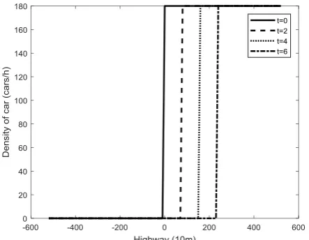
Problems B1 and B2 were examples of traffic flow, which were moving cars on the right followed by empty road behind. We called the position of traffic jam atx0. We obtained a shock wave moving to the right with positive speed.
Problem B1: Let us consider the initial condition
, 0 0, 0180, 0.
x x
x
(74)
This situation we obtain the velocity from (4),
80,38.528, .
x st v
x st
(75)
The exact solution of this problem is a shock wave of the form discussed in (68) and (69). The numerical solutions are shown in Fig. 5 and Fig. 6.
Fig. 5. Density of cars in 10 km highway for Problem B1 with 0.5
x
and t 0.001.
Fig. 6. Velocity of cars in 10 km highway for Problem B1 with 0.5
x
and t 0.001.
Problem B2: Let us consider the initial condition
, 0 40, 0 180, 0.x x
x
(76)
The corresponding numerical solutions are shown in Fig. 7 and Fig. 8.
Fig. 7. Density of cars in 10 km highway for Problem B2 with 0.5
x
and t 0.001.
Fig. 8. Velocity of cars in 10 km highway for Problem B2 with
0.5 x
and t 0.001.
From the numerical results, the empty road behind did not influence moving cars to the right. The solution was a shock with positive propagation speed, located at the end of the queue of cars; drivers braked and entered the congested region, where the car velocity smoothly decreased.
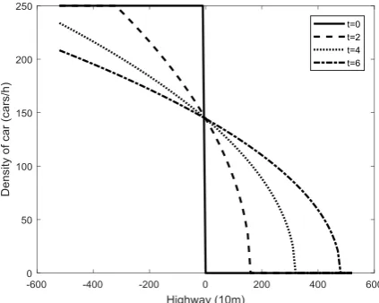
Suppose that traffic is lined up behind a red traffic light. We called the position of traffic lightx0 since the cars were bumper to bumper behind the traffic light. Assume that the cars are lined up indefinitely and of course, are not moving. If the light stops the traffic long enough, then we may also assume that there is no traffic ahead of the light.
Problems B3-B5 were examples of traffic flow that was similarly to red light situation. In the situation, cars start moving as light turns green. This means that cars located to the left are initially stationary but can begin to accelerate once the cars in front of them begin moving. The exact solution of these problems are a rarefaction wave of the form discussed in (70)-(73).
Problem B3: Let us consider the initial condition
IAENG International Journal of Applied Mathematics, 50:1, IJAM_50_1_29
[image:7.595.314.530.123.290.2] [image:7.595.57.279.337.509.2] [image:7.595.61.279.551.722.2]
, 0 180, 00, 0.
x x
x
(77) The corresponding numerical solutions are shown in Fig. 9 and Fig. 10.
Fig. 9. Density of cars in 10 km highway for Problem B3 with
0.5 x
and t 0.001.
Fig. 10. Velocity of cars in 10 km highway for Problem B3 with
0.5 x
and t 0.001.
Problem B4: Let us consider the initial condition
, 0 180, 0145, 0.
x x
x
(78) The corresponding numerical solutions are shown in Fig. 11 and Fig. 12.
Fig. 11. Density of cars in 10 km highway for Problem B4 with
0.5 x
and t 0.001.
Fig. 12. Velocity of cars in 10 km highway for Problem B4 with
0.5 x
and t 0.001.
Problem B5: Let us consider the initial condition
250, 0, 0
0, 0.
x x
x
(79)
The corresponding numerical solutions are shown in Fig. 13 and Fig. 14.
Fig. 13. Density of cars in 10 km highway for Problem B5 with
0.5 x
and t 0.001.
IAENG International Journal of Applied Mathematics, 50:1, IJAM_50_1_29
[image:8.595.312.523.60.229.2] [image:8.595.58.276.120.290.2] [image:8.595.317.529.271.436.2] [image:8.595.60.277.332.501.2] [image:8.595.316.528.561.730.2]Fig. 14. Velocity of cars in 10 km highway for Problem B5 with
0.5 x
and t 0.001.
From the numerical results, these problems described a traffic light controlling a junction. Since, behind the light a lot of cars arrived during the red light period. If the traffic light turned green, the cars behind the light accelerated until they reached the velocity fitting to the traffic situation ahead. We knew the flow at the traffic light, the number of
cars passing per hour is
max max
2 3 3v
t
. For a one-minute light, using max 250 vehicles/km and vmax80km/hour,
the number of cars of Problems B3-B5 would be about 128 cars.
VI. CONCLUSION
The traffic flow model based on non-linear velocity-density function, which is a quasi-linear first order partial differential equation, was used to predict the density and velocity profiles at the certain points of a highway 10 km after 6 minutes.
We found that the numerical solutions obtained by the upwind scheme (FTBS) and STG scheme converge to the exact solution and mean absolute errors tend to zero when the grid sizes xand t decrease. Moreover, the error of STG scheme was less than upwind scheme (FTBS). Therefore, the numerical results as shown in the figures were obtained by STG scheme.
Numerical simulations could verify the qualitative behavior of different flow variables in our models and the outcome of different situations of the model was presented. All problems of the numerical solutions for non-linear velocity density function were solved by STG scheme. The results showed that the density of cars increased while the velocity of cars decreased.
.
REFERENCES
[1] L.S Andallah, S. Ali, M.O. Gani, M.K. Pandit and J. Akhter, “A Finite Difference Scheme for a Traffic Flow Model on a Linear Velocity-Density Function,” Journal of Bangladesh Academy of Sciences, Vol. 32, No. 3, pp. 17-28, 2009. [2] M.O. Gani, M.M. Hossain and L.S. Andallah, “Lax- Friedrich
Scheme for Fluid Dynamic Traffic Flow Model Appended with Two-Point Boundary Condition,” GANIT J.Bangladesh Math. Soc., Vol. 31, pp. 43-52, 2011.
[3] C. Niyitegeka, Numerical Comparisons of Traffic Flow Models, Dissertation for the Degree of Master of Science, Department of Mathematics, Faculty of Science, TU Kaiserslautern and TU Eindhoven, 2012, pp. 2-25.
[4] H. Nessyahu and E. Tadmor, “Non-oscillatory Central Differencing for Hyperbolic Conservation Laws,” Journal of Computational Physics, Vol. 87, No. 2, pp.408-463, 1990. [5] M.H. Kabir, M.O. Gani and L.S. Andallah, “Numerical
Simulation of a Mathematical Traffic Flow Model Based on a Nonlinear Velocity-Density Function,” Journal of Bangladesh Academy of Sciences, Vol. 34, No. 1, pp. 15-22, 2010.
[6] M. Hasan, S. Sultana, L.S. Andallah, and T. Azam, “Lax-Friedrich Scheme for the Numerical Simulation of a Traffic Flow Model Based on a Nonlinear Velocity-Density Relation,” American Journal of Computational Mathematics,
Vol. 5, pp. 186-194, 2015.
[7] N. Chintaganon and W. Yomsatientkul, “Study on The Central Differencing Scheme with the Staggered Version (STG) for Solving the Hyperbolic Partial Differential Equations,” 17th International Conference on Mathematics, Statistics and Computational Sciences,
Tokyo Japan, pp. 3193-3197, 2015.
[8] Randall J. LeVeque, Numerical Methods for Conservation Laws, Washing-ton D.C., USA, 1992, pp. 28-31.
[9] Richard Haberman, Mathematical Model: Mechanical Vibrations, Population Dynamics, and Traffic Flow.
Prentice-Hall Inc.,Emglewood Cliffs, New Jersey, 1977, pp. 259-262.
Narumol Chintaganon is studying Ph.D. in Applied Mathematics, King Mongkut’s University of Technology Thonburi, Thailand.
Warisa Yomsatieankul graduated Ph.D. in Mathematics, 2010, Technische Universität Braunschweig, Germany and is currently lecturer at the department of Mathematics, KMUTT, Thailand.