Heuristic Based Backtracking for Propositional Satisfiability

Satisfiability

A. Bhalla, I. Lynce, J.T. de Sousa, and J. Marques-Silva

Technical University of Lisbon, IST/INESC-ID, Lisbon, Portugal {ateet,ines,jts,jpms}@sat.inesc.pt

Abstract. In recent years backtrack search algorithms for Propositional Satisfiability (SAT) have been the subject of dramatic improvements. These improvements allowed SAT solvers to successfully solve instances with thousands of variables and hundreds of thousands of clauses, and also motivated the development of many new challenging problem in-stances, many of which still too hard for the current generation of SAT solvers. As a result, further improvements to SAT technology are ex-pected to have key consequences in solving hard real-world instances. The objective of this paper is to propose heuristic approaches to the backtrack step of backtrack search SAT solvers, with the goal of increas-ing the ability of a SAT solver to search different parts of the search space. The proposed heuristics are inspired by the heuristics proposed in recent years for the branching step of SAT solvers, namely VSIDS and some of its improvements. Moreover, the completeness of the new algo-rithm is guaranteed. The preliminary experimental results are promising, and motivate the integration of heuristic backtracking in state-of-the-art SAT solvers.

1

Introduction

Propositional Satisfiability is a well-known NP-complete problem, with theoret-ical and practtheoret-ical significance, and with extensive applications in many fields of Computer Science and Engineering, including Artificial Intelligence and Elec-tronic Design Automation.

Current state-of-the-art SAT solvers incorporate sophisticated pruning tech-niques as well as new strategies on how to organize the search. Effective search pruning techniques are based, among others, on nogood learning and dependency-directed backtracking [16] and backjumping [5], whereas recent ef-fective strategies introduce variations on the organization of backtrack search. Examples of such strategies are weak-commitment search [17], search restarts [9] and random backtracking [10].

Advanced techniques applied to backtrack search SAT algorithms have achie-ved remarkable improvements [2,8,11,12], having been shown to be crucial for solving hard instances of SAT obtained from real-world applications. Moreover, and from a practical perspective, the most effective algorithms are complete,

Fernando Moura Pires, Salvador Abreu (Eds.): EPIA 2003, LNAI 2902, pp. 116–130, 2003. c

and so able to prove unsatisfiability. Indeed, this is often the objective in a large number of significant real-world applications.

Nevertheless, it is also widely accepted that local search can often have clear advantages with respect to backtrack search, since it is allowed to start the search over again whenever it gets stuck in a locally optimal partial solution. This advantage of local search has motivated the study of approaches for relax-ing backtrackrelax-ing conditions (while still assurrelax-ing completeness). The key idea is to unrestrictedly choose the point to backtrack to, in order to avoid thrashing during backtrack search. Moreover, one can think of combining different forms of relaxing the identification of the backtrack point.

In this paper, we propose to use heuristic knowledge to select the back-track point. Besides describing the generic heuristic backback-tracking search strat-egy, we establish backtracking heuristics inspired in the most promising branch-ing heuristics proposed in recent years, namely the VSIDS heuristic used by Chaff [12] and BerkMin’s branching heuristic [8]. Moreover, completeness con-ditions for the resulting SAT algorithm are established.

The remainder of this paper is organized as follows. The next section presents definitions used throughout the paper. Afterwards, we briefly survey backtrack search SAT algorithms. In Section 4 we introduce heuristic backtracking. Then, we describe unrestricted backtracking algorithms for SAT, and explain how heuristic backtracking can be regarded as a special case of unrestricted back-tracking. In addition, we address completeness issues. Next, Section 6 gives pre-liminary experimental results. Finally, we describe related work and conclude with directions for future research work.

2

Definitions

This section introduces the notational framework used throughout the paper. Propositional variables are denoted_x1, . . . , xn, and can be assigned truth values 0 (or_F) or 1 (or_T). The truth value assigned to a variable_xis denoted by_ν(_x). (When clear from context we use_x=_νx, where_νx∈ {0_,1}). A literal_l is either a variable_xior its negation¬_xi. A clause_ωis a disjunction of literals and a CNF formula_ϕ is a conjunction of clauses. A clause is said to besatisfiedif at least one of its literals assumes value 1, unsatisfied if all of its literals assume value 0, unitif all but one literal assume value 0, and unresolved otherwise. Literals with no assigned truth value are said to befree literals. A formula is said to be

satisfiedif all its clauses are satisfied, and is unsatisfiedif at least one clause is unsatisfied. A truth assignment for a formula is a set of pairs of variables and their corresponding truth values. The SAT problem consists of deciding whether there exists a truth assignment to the variables such that the formula becomes satisfied.

con-text, complete algorithms are often referred to assystematic, whereas incomplete algorithms are referred to asnon-systematic.

3

Backtrack Search SAT Algorithms

Over the years a large number of algorithms have been proposed for SAT, from the original Davis-Putnam procedure [4], to recent backtrack search al-gorithms [2,8,11,12] and to local search alal-gorithms [15], among many others.

The vast majority of backtrack search SAT algorithms build upon the original backtrack search algorithm of Davis, Logemann and Loveland [3]. The backtrack search algorithm is implemented by asearch processthat implicitly enumerates the space of 2npossible binary assignments to the_nproblem variables. Each dif-ferent truth assignment defines asearch pathwithin the search space. Adecision levelis associated with each variable selection and assignment. The first variable selection corresponds to decision level 1, and the decision level is incremented by 1 for each new decision assignment1_{. In addition, and for each decision level, the}

unit clause rule[4] is applied. (The iterated application of the unit clause rule is often referred to as Boolean Constraint Propagation (BCP)). If a clause is unit, then the sole free literal must be assigned value 1 for the formula to be satisfied. In this case, the value of the literal and of the associated variable are said to be

implied. Consequently, assigned variables can be distinguished betweendecision variablesandimplied variables.

In chronological backtracking, the search algorithm keeps track of which de-cision assignments have been toggled. Given an unsatisfied clause (i.e. aconflict

or a dead end) at decision level _d, the algorithm checks whether at the current decision level the corresponding decision variable _x has already been toggled. If not, the algorithm erases the variable assignments which are implied by the assignment on _x, including the assignment on _x, assigns the opposite value to x, and marks decision variable_x as toggled. In contrast, if the value of _xhas already been toggled, the search backtracks to decision level _d−1.

Recent state-of-the-art SAT solvers utilize different forms of non-chronological backtracking [2,11,12], in which each identified conflict is analyzed, its causes identified, and a new clause (nogood) created to explain and prevent the identified conflicting conditions. Created clauses are then used to compute the backtrack point as themost recentdecision assignment from all the decision assignments represented in the recorded clause. Moreover, some of the (larger) recorded clauses are eventually deleted. Clauses can be deleted opportunistically whenever they are no longerrelevantfor the current search path [11].

Figure 1 illustrates the differences between chronological backtracking (CB) and non-chronological backtracking (NCB). On the top of the figure appears a generic search tree (either possible in the context of CB or NCB). The search is performed accordingly to a depth-first search, and therefore the non-dashed branches define the search space explored so far. On the one hand, and when

1 _{Observe that all the assignments made before the first decision assignment}

CB(b)

NCB(a)

NCB(b) CB(a)

CB/NCB

Fig. 1.Chronological Backtracking (CB)vsNon-Chronological Backtracking (NCB)

a conflict if found, the chronological backtracking algorithm makes the search backtrack to the most recent yet untoggled decision variable (see CB(a)). On the other hand, when non-chronological backtracking is applied, the backtrack point is computed as the most recentdecision assignment from all the decision assignments represented in the recorded clause. In this case the search backtracks to a higher level in the search tree (NCB(a)), skipping portions of the search tree that are found to have no solution (see NCB(b)). From the final figures (CB(b) and NCB(b)) it is plain to conclude that the number of nodes explored by NCB is always equal or smaller than the number of nodes explored by CB2_{. (Observe} that nogoods can also reduce the search space, sincesimilarconflict paths of the search space are avoided to be searched.)

4

Heuristic Backtracking

Heuristic backtracking consists of selecting the backtrack point in the search tree as a function of variables in the most recently recorded clause. Different heuristics can be envisioned for applying heuristic backtracking. In this work we implemented three different heuristics:

1. One heuristic that decides the backtrack point given the information of the most recently recorded conflict clause.

2. Another heuristic that is inspired in the VSIDS branching heuristic, used by Chaff [12].

3. Finally, one heuristic that is inspired by BerkMin’s branching heuristic [8]. In all cases the backtrack point is computed as the variable with the largest heuristic metric.

Next, we describe how the three different approaches are implemented in the heuristic backtracking algorithm.

4.1 Plain Heuristic Backtracking

Under the plain heuristic backtracking approach the backtrack point (i.e. deci-sion level) is computed by selecting the decideci-sion level with the largest number of occurrences in the just recorded clause. After a conflict (i.e. an unsatisfied clause) is identified, aconflict clauseis created. The conflict clause is then used for heuristicallydeciding which decision assignment is to be toggled. This con-trasts with the usual non-chronological backtracking approach, in which the most recent decision assignment variable is selected as the backtrack point.

4.2 VSIDS-Like Heuristic Backtracking

The second approach to heuristic backtracking is based on the Variable State Independent Decaying Sum (VSIDS) branching heuristic [12]. VSIDS was the first of new generation of decision heuristics. This new heuristic has been used inChaff, a highly optimized SAT solver. More than to develop a well-behaviored heuristic, the motivation in Chaff has been to design a fast heuristic. In fact, one of the key properties of this strategy is the very low overhead, due to being independent of the variable state. As a result, the variable metrics are only updated when there is a conflict.

Similarly to Chaff, in VSIDS-like heuristic backtracking a metric is associ-ated with each literal, which is incremented when a new clause containing the literal; after every_kdecisions, the metric values are divided by a small constant. With the VSIDS-like heuristic backtracking, the assigned literal with the highest metric is selected as the backtrack point.

4.3 BerkMin-Like Heuristic Backtracking

In our implementation of BerkMin-like heuristic backtracking, the metrics of the literals of all clauses that are directly involved in producing the conflict, and so in creating the newly recorded clause, are updated when a clause is recorded. As in the cases of the VSIDS-like backtracking heuristic, the assigned literal with the highest metric is selected as the backtrack point.

5

Unrestricted Backtracking

Heuristic backtracking can be viewed as a special case of unrestricted backtrack-ing [10], the main difference bebacktrack-ing that while in unrestricted backtrackbacktrack-ing any form of backtrack step can be applied, in heuristic backtracking the backtrack point is computed from heuristic information, obtained from the current and past conflicts.

Unrestricted backtracking algorithms allow the search tounrestrictedly back-track to any point in the current search path whenever a conflict is reached. Besides the freedom for selecting the backtrack point in the decision tree, un-restricted backtracking entails apolicyfor applying different backtrack steps in sequence. Each backtrack step can be selected among chronological backtracking, non-chronological backtracking or incomplete forms of backtracking (e.g. search restarts, weak-commitment search, random backtracking, heuristic backtracking, among many others). More formally, unrestricted backtracking (UB) consists of defining a sequence of backtrack steps {BSt1,BSt2,BSt3, . . .} such that each backtrack step BSt_i can either be a chronological (CB), a non-chronological (NCB) or an incomplete form of backtracking (IFB).

Interestingly, the definition of unrestricted backtracking allows capturing the backtracking search strategies used by current state-of-the-art SAT solvers [2,8, 11,12]. Indeed, if the unrestricted backtracking strategy specifies always apply-ing the chronological backtrackapply-ing step or always applyapply-ing the non-chronological backtracking step, then we respectively capture the chronological and non-chronological backtracking search strategies.

Finally, observe that unrestricted backtracking gives a unified representa-tion for different backtracking strategies. Consequently, unrestricted backtrack-ing further allows establishbacktrack-ing general completeness conditions for classes of backtracking strategies and not only for each individual strategy, as it has often been done [14,17].

In what follows, we will further relate unrestricted backtracking with heuristic backtracking. In addition, we will describe completeness conditions established for unrestricted backtracking. We should note that the completeness conditions established to all organizations of unrestricted backtracking may obviously be applied to any special case of unrestricted backtracking (e.g. heuristic backtrack-ing).

5.1 Unrestricted Backtracking and Heuristic Backtracking

NCB

S

HB

S

?

CB

Fig. 2.Comparing Chronological Backtracking (CB), Non-Chronological Backtracking (NCB) and Heuristic Backtracking (HB)

step can be applied (CB, NCB or IFB), while in heuristic backtracking the backtrack point is heuristically selected.

Figure 2 exemplifies how heuristic backtracking can lead to incompleteness. Figure 2 illustrates the subsequent search of Figure 1, for both chronological (CB) and non-chronological backtracking (NCB). In addition, an example is given for heuristic backtracking (HB). The search path that leads to the solution is marked with letterS. For CB and NCB the solution is easily found. However, since with heuristic backtracking the search backtracks heuristically, the search space that leads to the solution is simply skipped. Hence, what has to be done in order to assure the correctness and completeness of the heuristic backtracking algorithm? First, and similarly to local search, we have to assume that the variable toggling in heuristic backtracking is reversible. For the given example, this means that the solution can be found in a subsequent search, although the solution would have been skipped if variable toggling was not reversible.

However, and exactly as with unrestricted backtracking, a number of tech-niques can be used to ensure completeness. These techtech-niques are analyzed in [10] and will be reviewed in what follows of this section. Completeness techniques for unrestricted backtracking can be organized in two classes:

– Marking recorded clauses as non-deletable. This solution may yield an ex-ponential growth in the number of recorded clauses3_.

– Increasing a given constraint (e.g. the number of non-deletable recorded causes) in between applications of different backtracking schemes. This solu-tion can be used to guarantee a polynomial growth of the number of recorded clauses.

5.2 Completeness Issues

In this section we address the problem of guaranteeing the completeness of SAT algorithms that implement some form of unrestricted backtracking (e.g. heuristic backtracking). It is clear that unrestricted backtracking can yield incomplete algorithms. Hence, for each newly devised SAT algorithm, that utilizes some form of UB, it is important to be able to apply conditions that guarantee the completeness of the resulting algorithm.

The results presented in this section generalize, for the unrestricted back-tracking algorithm, completeness results that have been proposed in the past

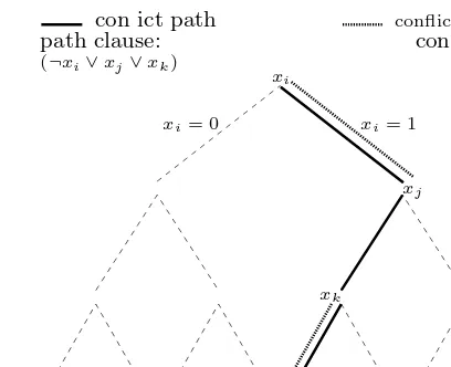
CONFLICT

xj

(¬x_i∨x_j∨x_k) path clause:con ict path

xi= 1

xi

conflict sub-path

xk

xi= 0

con ict clause: (¬xi∨xk)

Fig. 3.Search tree definitions

for specific backtracking relaxations. We start by establishing, in a more general context, a few already known results. Afterwards, we establish additional results regarding unrestricted backtracking.

In what follows we assume the organization of a backtrack search SAT algo-rithm as described earlier in this paper. The main loop of the algoalgo-rithm consists of selecting a variable assignment (i.e. adecision assignment), making that as-signment, and propagating that assignment using BCP. In the presence of an un-satisfied clause (i.e. aconflict) the algorithm backtracks to a decision assignment that can be toggled 4_{. Each time a conflict is identified, all the current decision} assignments define a conflict path in the search tree. (Observe that we restrict the definition of conflict path solely with respect to the decision assignments.) After a conflict is identified, we may apply a conflict analysis procedure [2,11, 12] to identify a subset of the decision assignments that represent a sufficient condition for producing the same conflict. The subset of decision assignments that is declared to be associated with a given conflict is referred to as aconflict sub-path. A straightforward conflict analysis procedure consists of constructing a clause withall the decision assignments in the conflict path. In this case the created clause is referred to as a path-clause. Figure 3 illustrates these defini-tions. We can now establish a few general results that will be used throughout this section.

Proposition 1. If an unrestricted backtracking search algorithm does not repeat conflict paths, then it is complete.

Proof. Assume a problem instance with_n variables. Observe that there are 2n possible conflict paths. If the algorithm does not repeat conflict paths, then it must necessarily terminate.

4 _{Without loss of generality, we assume that NCB also uses (binding) variable toggling}

Proposition 2. If an unrestricted backtracking search algorithm does not repeat conflict sub-paths, then it does not repeat conflict paths.

Proof. Observe that if a conflict sub-path is not repeated, then no conflict path can contain the same sub-path, and so no conflict path can be repeated.

Proposition 3. If an unrestricted backtracking search algorithm does not repeat conflict sub-paths, then it is complete.

Proof. Given the two previous results, if no conflict sub-paths are repeated, then no conflict paths are repeated, and so completeness is obtained.

Proposition 4. If the number of times an unrestricted backtracking search algo-rithm repeats conflict paths or conflict sub-paths is upper-bounded by a constant, then the backtrack search algorithm is complete.

Proof. We prove the result for conflict paths; for conflict sub-paths, it is similar. Let_M be a constant denoting an upper bound on the number of times a given conflict path can be repeated. Since the total number of distinct conflict paths is 2n, and since each can be repeated at most _M times, then the total number of conflict paths the backtrack search algorithm can enumerate is_M ×2n, and so the algorithm is complete.

Proposition 5. For an unrestricted backtracking search algorithm the following holds:

1. If the algorithm creates a path clause for each identified conflict, then the search algorithm repeats no conflict paths.

2. If the algorithm creates a conflict clause for each identified conflict, then the search algorithm repeats no conflict sub-paths.

3. If the algorithm creates a conflict clause (or a path clause) after every

M identified conflicts, then the number of times an unrestricted backtrack-ing search algorithm repeats conflict sub-paths (or conflict paths) is upper-bounded.

In all of the above cases, the search algorithm is complete.

Observe that Proposition 5 holds independently of which backtrack step is taken each time a conflict is identified. Hence, as long as we record a conflict for each identified conflict,anyform of unrestricted backtracking yields a complete algorithm. Less general formulations of this result have been proposed in the recent past [6,17,14].

The results established so far guarantee completeness at the cost of recording (and keeping) a clause for each identified conflict. In this section we propose and analyze conditions for relaxing this requirement. As a result, we allow for some clauses to be deleted during the search process, and only require some specific recorded clauses to be kept5_{. (We should note that clause deletion does} not apply to chronological backtracking strategies and that, as shown in [11], existing clause deletion policies for non-chronological backtracking strategies do not compromise the completeness of the algorithm.) Afterwards, we propose other conditions that do not require specific recorded clauses to be kept.

Proposition 6. An unrestricted backtracking algorithm is complete if it records (and keeps) aconflict-clausefor each identified conflict for which an IFB step is taken.

Proof. Observe that there are at most 2n IFB steps that can be taken, because a conflict clause is recorded for each identified conflict for which an IFB step is taken, and so conflict sub-paths due to IFB steps cannot be repeated. Moreover, the additional backtrack steps that can be applied (CB and NCB) also ensure completeness. Hence, the resulting algorithm is complete.

Moreover, we can also generalize Proposition 4.

Proposition 7. Given an integer constant_M, an unrestricted backtracking al-gorithm is complete if it records (and keeps) a conflict-clause after every _M identified conflicts for which an IFB step is taken.

Proof. The result immediately follows from Propositions 5 and 6.

As one final remark, observe that for the previous conditions, the number of recorded clauses grows linearly with the number of conflicts where an IFB step is taken, and so in the worst-case exponentially in the number of variables.

Other approaches to guarantee completeness involve increasing the value of some constraint associated with the search algorithm. The following results il-lustrate these approaches.

Proposition 8. Suppose an unrestricted backtracking strategy that applies a se-quence of backtrack steps. If for this sese-quence the number of conflicts in between IFB steps strictly increases after each IFB step, then the resulting algorithm is complete.

5 _{We say that a recorded clause is kept provided it is prevented from being deleted}

Proof. If only CB or NCB steps are taken, then the resulting algorithm is com-plete. When the number of conflicts in between IFB steps reaches 2n, the algo-rithm is guaranteed to terminate.

We should also note that this result can be viewed as a generalization of the completeness-ensuring condition used in search restarts, that consists of increas-ing the backtrack cutoff value after each search restart [1]6. Finally, observe that in this situation the growth in the number of clauses can be made polynomial, provided clause deletion is applied on clauses recorded from NCB and IFB steps. The next result establishes conditions for guaranteeing completeness when-ever large recorded clauses (due to an IFB step) are opportunistically deleted. The idea is to increase the size of recorded clauses that are kept after each IFB step. Another approach is to increase the life-span of large-recorded clauses, by increasing the relevance-based learning threshold [2].

Proposition 9. Suppose an unrestricted backtracking strategy that applies a specific sequence of backtrack steps. If for this sequence, either the size of the largest recorded clause kept or the size of the relevance-based learning threshold is strictly increased after each IFB step is taken, then the resulting algorithm is complete.

Proof. When either the size of the largest recorded clause reaches value _n, or the relevance-based learning threshold reaches value_n, all recorded clauses will be kept, and so completeness is guaranteed from Proposition 5.

Observe that for this last result the number of clauses can grow exponentially with the number of variables. Moreover, we should note that the observation regarding increasing the relevance-based learning threshold was first suggested in [12].

One final result addresses the number of times conflict paths and conflict sub-paths can be repeated.

Proposition 10. Under the conditions of Proposition 8 and Proposition 9, the number of times a conflict path or a conflict sub-path is repeated is upper-bounded.

Proof. Clearly, the resulting algorithms are complete, and so known to terminate after a maximum number of backtrack steps (that is constant for each instance). Hence, the number of times a conflict path (or conflict sub-path) can be repeated is necessarily upper-bounded.

6

Experimental Results

This section presents the experimental results of applying heuristic backtracking to different classes of problem instances. In addition, we compare heuristic back-tracking with other forms of backback-tracking relaxations, namely search restarts [9]

and random backtracking [10]. Our goal here has been to test the feasibility of the heuristic backtracking algorithm using three different heuristics: a plain heuris-tic, the VSIDS heuristic and the BerkMin’s heuristic. Experimental evaluation of the different algorithms has been done using the JQUEST SAT framework, a Java framework for prototyping SAT algorithms. All the experiments were run on the same P4/1.7GHz/1GByte of RAM/Linux machine. The CPU time limit for each instance was set to 2000 seconds, except for instances from Bei-jing family, for which the maximum run time allowed was 5000 seconds. In all cases where the algorithm was unable to solve an instance it was due to memory exhaustion.

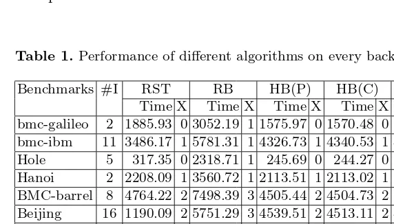
The total run times for solving different class of benchmarks are shown in Table 1 and Table 2. In both tables,#Idenotes the number of problem instances,

Timedenotes the CPU time andXdenotes the number of aborted instances. In addition, each column indicates a different form of backtracking relaxation:

– RST indicates that the search restart strategy [9] is applied with a cutoff value of 100 backtracks and is kept fixed. All recorded clauses are kept to ensure completeness.

– RB indicates that random backtracking [10] is applied at each backtrack step.

– HB(P) indicates that plain heuristic backtracking is applied at each back-track step.

– HB(C) indicates that the Chaff’s VSIDS-like heuristic backtracking is ap-plied at each step.

– HB(B) indicates that the BerkMin-like heuristic backtracking is applied at each step.

Table 1.Performance of different algorithms on every backtrack step.

Benchmarks #I RST RB HB(P) HB(C) HB(B)

Table 2.Performance of different algorithms on every 100 backtracks.

Benchmarks #I RST RB HB(P) HB(C) HB(B)

Time X Time X Time X Time X Time X bmc-galileo 2 1833.57 0 2242.93 0 527.14 0 359.22 0 414.57 0 bmc-ibm 11 4553.88 1 4585.39 1 4796.98 1 3989.88 1 4166.41 1 Hole 5 356.44 0 284.9 0 355.71 0 356.6 0 338.57 0 Hanoi 2 2122.98 1 2058.92 1 2183.49 1 2239.5 1 2235.25 1 BMC-barrel 8 4824.22 2 4742.33 2 7521.81 3 6840.03 3 7402.13 3 Beijing 16 5768.92 2 3822.52 2 3555.38 2 3369.57 2 4642.97 2 Blocksworld 7 933.18 0 526.19 0 613.31 0 1092.62 0 1448.54 0 Logistics 4 14.76 0 14.27 0 10.98 0 10.47 0 11.82 0 par16 10 895.83 0 829.68 0 292.77 0 334.4 0 382.55 0 ii16 10 38.3 0 55.49 0 135.86 0 132.85 0 138.61 0 ucsc-ssa 102 33.9 0 46.79 0 36.17 0 35.25 0 49.02 0 ucsc-bf 223 90.7 0 112.01 0 87.23 0 64.67 0 111.95 0

In Table 1, the different forms of backtracking are performed at every back-track step. In addition, completeness is ensured by marking the recorded clauses as non-deletable. In Table 2, the different forms of backtracking are performed after every 100 backtracks, and an increment of 10 backtracks is applied. In this case, completeness is ensured by marking clauses recorded whenever a relaxed backtrack step is performed as non-deletable.

As can be concluded from the experimental results, heuristic backtracking can yield significant savings in CPU time, and also allow for a smaller number of instances to be aborted. This is true for several of the classes of problem instances analyzed.

7

Related Work

Dependency-directed backtracking and nogood learning were originally proposed by Stallman and Sussman in [16] in the area of Truth Maintenance Systems (TMS). In the area of Constraint Satisfaction Problems (CSP), the topic was independently studied by J. Gaschnig [5] and others (see for example [13]) as different forms of backjumping.

arbitrary search movement [7], starting withany complete assignmentand evolv-ing by flippevolv-ing values of variables obtained from the conflicts.

In weak-commitment search [17], the algorithm constructs a consistent partial solution, but commits to the partial solutionweakly. In weak-commitment search, whenever a conflict is reached, thewholepartial solution is abandoned, in explicit contrast to standard backtracking algorithms where the most recently added variable is removed from the partial solution.

Moreover, search restarts have been proposed and shown effective for hard instances of SAT [9]. The search is repeatedly restarted whenever a cutoff value is reached. The algorithm proposed is not complete, since the restart cutoff point is kept constant. In [1], search restarts were jointly used with learning for solving hard real-world instances of SAT. This latter algorithm is complete, since the backtrack cutoff value increases after each restart. One additional example of backtracking relaxation is described in [14], which is based on attempting to construct a complete solution, that restarts each time a conflict is identified. More recently, highly-optimized complete SAT solvers [8,12] have successfully combined non-chronological backtracking and search restarts, again obtaining remarkable improvements in solving real-world instances of SAT.

8

Conclusions and Future Work

This paper proposes the utilization of heuristic backtracking in backtrack search SAT solvers. The most well-known branching heuristics used in state-of-the-art SAT solvers were adapted to the backtrack step of SAT solvers. The experimental results illustrate the practicality of heuristic backtracking.

The main contributions of this paper can be summarized as follows: 1. A new heuristic backtrack search SAT algorithm is proposed, that

heuristi-cally selects the point to backtrack to.

2. The proposed SAT algorithm is shown to be a special case of unrestricted backtracking, and different approaches for ensuring completeness are de-scribed.

3. Experimental results indicate that significant savings in search effort can be obtained for different organizations of the proposed heuristic backtrack search algorithm.

Besides the preliminary experimental results, a more comprehensive experi-mental evaluation is required. In addition, future work entails deriving conditions for selecting among search restarts and heuristic backtracking.

References

2. R. Bayardo Jr. and R. Schrag. Using CSP look-back techniques to solve real-world SAT instances. InProceedings of the National Conference on Artificial Intelligence, pages 203–208, July 1997.

3. M. Davis, G. Logemann, and D. Loveland. A machine program for theorem-proving.Communications of the Association for Computing Machinery, 5:394–397, July 1962.

4. M. Davis and H. Putnam. A computing procedure for quantification theory. Jour-nal of the Association for Computing Machinery, 7:201–215, July 1960.

5. J. Gaschnig. Performance Measurement and Analysis of Certain Search Algo-rithms. PhD thesis, Carnegie-Mellon University, Pittsburgh, PA, May 1979. 6. M. Ginsberg. Dynamic backtracking. Journal of Artificial Intelligence Research,

1:25–46, 1993.

7. M. Ginsberg and D. McAllester. GSAT and dynamic backtracking. InProceedings of the International Conference on Principles of Knowledge and Reasoning, pages 226–237, 1994.

8. E. Goldberg and Y. Novikov. BerkMin: a fast and robust sat-solver. InProceedings of the Design and Test in Europe Conference, pages 142–149, March 2002. 9. C. P. Gomes, B. Selman, and H. Kautz. Boosting combinatorial search through

randomization. InProceedings of the National Conference on Artificial Intelligence, pages 431–437, July 1998.

10. I. Lynce and J. P. Marques-Silva. Complete unrestricted backtracking algorithms for satisfiability. In Proceedings of the International Symposium on Theory and Applications of Satisfiability Testing, pages 214–221, May 2002.

11. J. P. Marques-Silva and K. A. Sakallah. GRASP-A search algorithm for proposi-tional satisfiability. IEEE Transactions on Computers, 48(5):506–521, May 1999. 12. M. Moskewicz, C. Madigan, Y. Zhao, L. Zhang, and S. Malik. Engineering an

efficient SAT solver. InProceedings of the Design Automation Conference, pages 530–535, June 2001.

13. Patrick Prosser. Hybrid algorithms for the constraint satisfaction problems. Com-putational Intelligence, 9(3):268–299, August 1993.

14. E. T. Richards and B. Richards. Non-systematic search and no-good learning.

Journal of Automated Reasoning, 24(4):483–533, 2000.

15. B. Selman and H. Kautz. Domain-independent extensions to GSAT: Solving large structured satisfiability problems. In Proceedings of the International Joint Con-ference on Artificial Intelligence, pages 290–295, August 1993.

16. R. M. Stallman and G. J. Sussman. Forward reasoning and dependency-directed backtracking in a system for computer-aided circuit analysis.Artificial Intelligence, 9:135–196, October 1977.