Mixed of Elzaki Transform and Projected Differential Transform Method for a Nonlinear Wave-Like Equations with Variable Coefficients

(1)

MIXED OF ELZAKI TRANSFORM AND PROJECTED DIFFERENTIAL TRANSFORM METHOD FOR A NONLINEAR WAVE-LIKE EQUATIONS WITH VARIABLE

COEFFICIENTS

A. KHALOUTA1 _{AND A. KADEM}2

Abstract. In this work, a mixture of Elzaki transform and projected di¤erential transform method is applied to solve a nonlinear wave-like equations with variable coe¢ cients. Nonlinear terms can be easily ma-nipulated by using the projected di¤erential transformation method. The method gives the results show that the proposed method is very e¢ cient, simple and can be applied to other applications.

1. Introduction

The integral transforms play a signi…cant role in many …elds of science and in the literature, it’s are largely used in mathematical physics, optics, mathematical engineering and in some others in order to solve the di¤erential equations such as Laplace, Fourier, Mellin, Hankel and Sumudu.

Recently, Tarig Elzaki [5] introduced a new integral transform, called Elzaki transform, which is applied to solve an ordinary and partial di¤eren-tial equations.

By applying the Adomian decomposition method (ADM), M. Ghoreishi solved some types of nonlinear wave-like equation [6], V.G. Gupta and S. Gupta worked out by using homotopy perturbation transform method ( HPTM) these types of equation tool [7], furthermore, A. Aslanov [3], F. Yin and et al [12] and A. Atangana and et al [2] researched for solving nonlin-ear heat and wave-like equation by using homotopy perturbation, variational iteration and homotopy decomposition methods respectively. Moreover, var-ious techniques, such as homotopy analysis, perturbations, decompositions, iterations, di¤erential and Laplace transformation techniques have been used to handle similar types of these wave-like and also heat-like problems nu-merically and analytically as in references [1],[7],[10],[11].

In this work, we will present the mixed of Elzaki transform and projected di¤erential transform method, in order to solve a nonlinear wave-like equa-tions. This method called Elzaki projected di¤erential transform method (EPDTM).

2010 Mathematics Subject Classi…cation. Primary 35L05, 35L10; Secondary 35A22, 35A35.

Key words and phrases. Nonlinear wave-like equations, Elzaki transform, Projected di¤erential transform method.

1

(2)

Consider the following nonlinear wave-like equations

@2u @t2 =

n

X

i;j=1

F1ij(X; t; u)

@k+m

@xk_i@xm_j F2ij(uxi; uxj)

+

n

X

i=1

G1i(X; t; u)

@p

@xp_iG2i(uxi) +H(X; t; u) +S(X; t);

with the initial conditions

u(X;0) =a0(X); ut(X;0) =a1(X):

Here X = (x1; x2; :::; xn); F1ij; G1i i; j 2 f1;2; :::; ng are nonlinear func-tions of X; t and u; F2ij; G2i i; j 2 f1;2; :::; ng; are nonlinear functions of derivatives of u with respect to xi and xj i; j 2 f1;2; :::; ng; respectively. Also H; S are nonlinear functions and k; m; pare integers.

These types of equations are of considerable signi…cance in various …elds of applied sciences, mathematical physics, nonlinear hydrodynamics, engineer-ing physics, biophysics, human movement sciences, astrophysics and plasma physics. These equations describe the evolution of erratic motions of small particles that are immersed in ‡uids, ‡uctuations of the intensity of laser light, velocity distributions of ‡uid particles in turbulent ‡ows.

2. Elzaki transform

De…nition 2.1. A new integral transform called Elzaki transform [4],[5]

de…ned for functions of exponential order, is proclaimed. We consider func-tions in the set A de…ned by,

A= f(t)=₉M; k1; k2 >0;jf(t)j< M e

jtj

kj_; _if _t₂_{( 1)}j _[0_; 1) :

Elzaki transform of the function f(t) is

E[f(t)] =T(v) =v

Z ₁

0

f(t)e vtdt; t >0;

where v is the factor of variable t.

T. M. Elzaki and S. M. Elzaki in [4], showed the modi…ed of Sumudu transform [9] or Elzaki transform was applied to partial di¤erential equa-tions, ordinary di¤erential equaequa-tions, system of ordinary and partial di¤er-ential equations and integral equations.

Proposition 2.2. To obtain Elzaki transform of partial derivative we use integration by parts and then we have

E @f(x; t)

@t =

1

vT(x; v) vf(x;0);

E @f(x; t)

@x =

d

dx[T(x; v)];

E @

2_f₍_{x; t}₎

@t2 =

1

v2T(x; v) f(x;0) v

@f(x;0) @t ;

E @

2_f₍_{x; t}₎

@x2 =

d2

(3)

Proof.

E @f(x; t)

@t =

Z ₁

0 v@f

@te t

vdt= lim

p!1

Z p

0

ve vt @f @tdt

= lim

p!1

h

ve vtf(x; t) ip

0 Z p

0

e vtf(x; t)dt

= 1

vT(x; v) vf(x;0):

We assume that f is piecewise continuous and it is of exponential order. Now

E @f(x; t)

@x =

Z ₁

0

ve vt @f(x; t) @x dt=

@ @x

Z ₁

0

ve vtf(x; t)dt;

using the Leibniz rule to …nd

E @f(x; t)

@x =

d

dx[T(x; v)]:

By the same method we …nd

E @

2_f₍_{x; t}₎

@x2 = d2

dx2[T(x; v)];

and

E @

2_f₍_{x; t}₎

@t2

Let

@f @t =g;

then we have

E @

2_f₍_{x; t}₎

@t2 = E

@g(x; t)

@t =

1

vE[g(x; t)] vg(x;0)

= 1

v2T(x; v) f(x;0) v

@f(x;0) @t :

We can easily extend this result to the n th partial derivative by using mathematical induction, we have

E @

n_f₍_{x; t}₎

@tn =

1

vnT(x; v) n 1 X

k=0

v2 n+k@

k_f₍_x;₀₎

@tk :

The proof is complete.

Properties of Elzaki transform can be found in [4],[5] we mention only the following

E(1) = v2;

(4)

3. Projected di¤erential transform method

In this section, we introduce the basic idea of modi…ed version of the di¤erential transform method (DTM), the projected di¤erential transform method (PDTM) [8]. The DTM is based on the Taylor series for all variables. Here, we consider the Talyor series of the function u with respect to the speci…c variable. Assume that the speci…c variable is the variable t.

De…nition 3.1. The projected di¤ erential transform U(X; k) of u(X; t) with respect to the variable t at t0 is de…ned by

(3.1) U(X; k) = 1 k!

@k

@tku(X; t) t=t0

;

where X = (x1; x2; :::; xn); u(X; t) is the original function and U(X; k) is

the transformed function of u(X; t).

De…nition 3.2. The projected di¤ erential inverse transform ofU(X; k)with respect to the variable t att0 is de…ned by

(3.2) u(X; t) =

1

X

k=0

U(X; k)(t t0)k:

Combining Eqs. (3.1) and (3.2), we have the Taylor series expansion of the function u att=t0 as follows

(3.3) u(X; t) =

1

X

k=0 1 k!

@k

@tku(X; t) t=t0

(t t0)k:

From the above de…nitions, the fundamental operations of the PDTM are given by the following theorems

Theorem 3.3. Let U(X; k); W(X; k) and Z(X; k) be the projected di¤ er-ential transform of the functions u(X; t); w(X; t) and z(X; t) respectively, where X= (x1; x2; :::; xn); then

(1) if

z(X; t) = u(X; t) + w(X; t);

then

Z(X; k) = U(X; k) + W(X; k);

where and are constants.

(2) if

z(X; t) =u(X; t)w(X; t);

then

Z(X; k) =

k

X

r=0

U(X; r)W(X; k r) =

k

X

r=0

W(X; r)U(X; k r):

(3) if

(5)

then

Z(X; k) =

k

X

kn 1=0 k_Xn 1 kn 2=0

:::

k3

X

k2=0

k2

X

k1=0

U1(X; k1)U2(X; k2 k1)

::: Un 1(X; kn 1 kn 2)Un(X; k kn 1):

(4) if

z(X; t) = @

n

@tnu(X; t);

then

Z(X; k) = (k+ 1)(k+ 2):::(k+n)U(X; k+n)

= (k+n)!

k! U(X; k+n); n2 f1;2; :::g:

(5) if

z(X; t) = @

n

@xn i

u(x1; x1; :::; xn; t);

then

Z(X; k) = @

n

@xn i

U(x1; x1; :::; xn; k);

i _{2 f}1;2; :::; n_g; n_{2 f}1;2; :::_g:

(6) if

z(X; t) =xa1₁ xa2₂ :::xan

n tam;

then

Z(X; k) =xa1₁ xa2₂ :::xan

n (km am) =

xa1₁ xa2₂ :::xan

n ; km=am

0; otherwise :

(7) if

z(X; t) =xa1₁ xa2₂ :::xan

n tamu(X; t);

then

Z(X; k) =xa1₁ xa2₂ :::xan

n U(X; k n):

4. EPDTM for nonlinear wave-like equations

In this section we describe the application of the Elzaki projected di¤er-ential transform method (EPDTM) for nonlinear wave-like equations with initial conditions.

Theorem 4.1. Consider the nonlinear wave-like equations @2u

@t2 =

n

X

i;j=1

F1ij(X; t; u)

@k+m

(4.1)

+

n

X

i=1

G1i(X; t; u)

@p

@xp_iG2i(uxi) +H(X; t; u) +S(X; t);

with the initial conditions

(6)

Here X = (x1; x2; :::; xn); F1ij; G1i i; j 2 f1;2; :::; ngare nonlinear functions

of X; t and u; F2ij; G2i i; j 2 f1;2; :::; ng; are nonlinear functions of

deriv-atives of u with respect to xi and xj i; j 2 f1;2; :::; ng; respectively. Also

H; S are nonlinear functions andk; m; p are integers.

Then by EPDTM we have the solution of Eqs. (4.1) with initial condi-tion (4.2) in the form of in…nite series which converge rapidly to the exact solution as follows

u(X; t) =

1

X

k=0

U(X; k);

where U(X; k) is projected transform function of u(X; t):

Proof. In order to to achieve our goal, we consider the following nonlinear wave-like Eqs. (4.1) with the initial conditions (4.2).

First, we take the Elzaki transform on both sides of (4.1) subject to initial conditions (4.2), we get

E @ 2_u

@t2 = E 2 4

n

X

i;j=1

F1ij(X; t; u)

@k+m @xk

i@xmj

F2ij(uxi; uxj)

+

n

X

i=1

G1i(X; t; u)

@p

@xp_iG2i(uxi) +H(X; t; u) #

+E[S(X; t)]:

(4.3)

Using the di¤erentiation property of Elzaki transforms2.2and above initial conditions, we have

E[u(X; t)] = v2u(X;0) +v3ut(X;0) +v2E[S(X; t)]

+v2E 2 4

n

X

i;j=1

F1ij(X; t; u)

@k+m

(4.4)

+

n

X

i=1

G1i(X; t; u)

@p

@xp_iG2i(uxi) +H(X; t; u) #

:

Applying the inverse Elzaki transform on both sides of Eq. (4.4), to …nd

u(X; t) = L(X; t) +E 1 0 @v2E

2 4

n

X

i;j=1

F1ij(X; t; u)

@k+m @xk

i@xmj

F2ij(uxi; uxj)

+

n

X

i=1

G1i(X; t; u)

@p

@xp_iG2i(uxi) +H(X; t; u) #!

;

(4.5) where

L(X; t) = E 1 v2u(X;0) +v3ut(X;0) +v2E[S(X; t)]

= a0(X) +ta1(X) +E 1 v2E[S(X; t)]

represents the term arising from the source term and the prescribed initial conditions.

Now, we apply the projected di¤erential transform method.

U(X;0) = L(X; t);

(7)

U(X; k+ 1) = E 1 v2E[A(X; k) +B(X; k) +C(X; k)] ;

where A(X; k); B(X; k) and C(X; k) are the projected di¤erential trans-formed form of the nonlinear terms of

n

P

i;j=1

F1ij(X; t; u) @

k+m

@xk i@xmj

F2ij(uxi; uxj);

n

P

i=1

G1i(X; t; u) @

p

@xp_iG2i(uxi);and H(X; t; u):

From Eq. (4.6), we have

U(X;0) = L(X; t);

U(X;1) = E 1 v2E[A(X;0) +B(X;0) +C(X;0)] ;

U(X;2) = E 1 v2E[A(X;1) +B(X;1) +C(X;1)] ;

U(X;3) = E 1 v2E[A(X;2) +B(X;2) +C(X;2)] ;

::::

and so on.

Then, the solution of Eqs. (4.1) and (4.2) is given as follows

u(X; t) =

1

X

k=0

U(X; k):

The proof is complete.

To illustrate the capability and simplicity of the method, some examples for nonlinear partial di¤erential equations will be discussed in particular nonlinear wave-like equations.

5. Numerical Application

In this section, we apply mixture of Elzaki transform and the projected di¤erential transform method for solving various types of nonlinear wave-like equations with variable coe¢ cients and we compare the approximate analytical solution obtained for our nonlinear wave-like problems with known exact solutions .

Example 1Consider the 2-dimensional nonlinear wave-like equation with variable coe¢ cients

(5.1) @

2_u

@t2 = @2

@x@y(uxxuyy) @2

@x@y(xyuxuy) u;

with initial conditions

(5.2) u(x; y;0) =exy; ut(x; y;0) =exy;

where u=u(x; y; t) is a …eld function, (x; y; t)₂_R _R _R+: The exact solution to (5.1) with initial conditions (5.2) is given by

u(x; y; t) =exy(sint+ cost):

By taking Elzaki transformon on both sides of (5.1) subject to initial con-ditions (5.2), and using the proposition 2.2, we obtain

E[u(x; y; t)] = v2exy+v3exy

(8)

+v2E @ 2

@x@y(uxxuyy) @2

@x@y(xyuxuy) u :

By applying the inverse Elzaki transform for (5.3), we get

u(x; y; t) = exy+texy

+E 1 v2E @ 2

@x@y(uxxuyy) @2

@x@y(xyuxuy) u :

Applying projected di¤ erential transform method to obtain

U(x; y; k+ 1) = E 1 v2E @ 2

@x@yA(x; y; k) @2

@x@yxyB(x; y; k) u(x; y; k)]);

(5.4)

with

(5.5) U(x; y;0) =exy+texy;

where A(x; y; k) and B(x; y; k) are the projected di¤ erential transformed of the nonlinear terms,uxxuyy and uxuy having the value

A(x; y; k) =

k

X

r=0

@2U(x; y; r) @x2

@2U(x; y; k r) @y2 ;

B(x; y; k) =

k

X

r=0

@U(x; y; r) @x

@U(x; y; k r)

@y :

The few nonlinear terms are as follows

A(0) = Uxx(0)Uyy(0);

A(1) = Uxx(0)uyy(1) +Uxx(1)Uyy(0);

A(2) = uxx(0)uyy(2) +uxx(1)uyy(1) +uxx(2)uyy(0)

:::;

and so on.

B(0) = Ux(0)Uy(0);

B(1) = Ux(0)Uy(1) +Ux(1)Uy(0);

B(2) = Ux(0)uy(2) +Ux(1)uy(1) +Ux(2)Uy(0)

:::;

and so on.

From the relationship in (5.4),(5.5), we obtain

U(x; y;0) = exy+texy = (1 +t)exy;

U(x; y;1) = E 1 v2E @ 2

@x@yA(x; y;0) @2

@x@yxyB(x; y;0) u(x; y;0)

= t

2

2! t3 3! e

xy_;

U(x; y;2) = E 1 v2E @ 2

@x@yA(x; y;1) @2

(9)

= t 4 4! + t5 5! e xy_;

U(x; y;3) = E 1 v2E @ 2

@x@yA(x; y;2) @2

@x@yxyB(x; y;2) u(x; y;2)

= t 6 6! t7 7! e xy_; :::;

and so on.

Which in closed form gives exact solution

u(x; y; t) =

1

X

k=0

U(x; y; k) = 1 +t t 2 2! t3 3!+ t4 4! + t5 5! t6 6! t7

7!+::: e

xy

= (sint+ cost)exy:

which is an exactly the same solution obtained by Adomian decomposition method [6] and Homotopy perturbation transform method [7] for the same test problem.

Example 2 Consider the following nonlinear wave-like equation with variable coe¢ cients

(5.6) @

2_u

@t2 =u 2 @2

@x2(uxuxxuxxx) +u 2

x

@2 @x2(u

3

xx) 18u5+u;

(5.7) u(x;0) =ex; ut(x;0) =ex;

where u=u(x; t) is a …eld function, (x; t)₂]0;1[ _R+:

The exact solution to (5.6) with initial conditions (5.7) is given by

u(x; t) =ex+t:

By taking Elzaki transform on both sides of (5.6) subject to initial condi-tions (5.7), and using the proposition 2.2, we obtain

E[u(x; t)] = v2ex+v3ex

+v2E u2 @ 2

@x2(uxuxxuxxx) +u 2

x

@2 @x2(u

3

xx) 18u5+u

u(x; t) = ex+tex

+E 1 v2E u2 @ 2

@x2(uxuxxuxxx) +u 2

x

@2 @x2(u

3

xx) 18u5+u :

(5.8) U(x; k+ 1) =E 1 v2E[A(x; k) +B(x; k) 18C(x; k) +u(x; k)] ; with

(5.9) U(x;0) =ex+tex;

where A(x; k); B(x; k)and C(x; k)are the projected di¤ erential transformed of the nonlinear terms u2 @2

@x2(uxuxxuxxx); u2x @ 2

(10)

A(x; k) = k X r=0 r X s=0 s X m=0 m X n=0

U(x; n)U(x; m n)

@2 @x2

@U(x; s m) @x

@2U(x; r s) @x2

@3U(x; k r)

@x3 ;

B(x; k) =

k X r=0 r X s=0 s X m=0 m X n=0

@U(x; n) @x

@U(x; m n) @x

@2 @x2

@2U(x; s m) @x2

@2U(x; r s) @x2

@2U(x; k r)

@x2 ;

C(x; k) =

k X r=0 r X s=0 s X m=0 m X n=0

U(x; n)U(x; m n)U(x; s m)

U(x; r s)U(x; k r):

A(0) = U2(0) @ 2

@x2 [Ux(0)Uxx(0)Uxxx(0)];

A(1) = 2U(0)U(1) @ 2

@x2 [Ux(0)Uxx(0)Uxxx(0)] +U

2₍₀₎ @2

@x2[Ux(1)Uxx(0)Uxxx(0) +Ux(0)Uxx(1)Uxxx(0) +Ux(0)Uxx(0)Uxxx(1)]

:::;

and so on.

B(0) = U_x2(0) @ 2

@x2U 3

xx(0);

B(1) = 2Ux(0)Ux(1)

@2 @x2U

3

xx(0) + 3Ux2(0)

@2 @x2 U

2

xx(0)Uxx(1) ;

:::;

and so on.

C(0) =U5(0); C(1) = 5U4(0)U(1); ::::;

and so on.

U(x;0) = ex+tex = (1 +t)ex;

U(x;1) = E 1 v2E[A(x;0) +B(x;0) 18C(x;0) +u(x;0)]

= t 2 2!+ t3 3! e x_;

U(x;2) = E 1 v2E[A(x;1) +B(x;1) 18C(x;1) +u(x;1)]

= t 4 4!+ t5 5! e x_; :::;

(11)

u(x; t) =

1

X

k=0

U(x; k) = 1 +t+ t 2

2!+ t3 3! +

t4 4!+

t5

5! +::: e

x

= ex+t:

Example 3 Consider the following one dimensional nonlinear wave-like equation with variable coe¢ cients

(5.10) @

2_u

@t2 =x 2 @

@x(uxuxx) x 2₍_u2

xx) u;

(5.11) u(x;0) = 0; ut(x;0) =x2;

where u=u(x; t) is a …eld function, (x; t)₂]0;1[ _R+_:

The exact solution to (5.10) with initial conditions (5.11) is given by

u(x; t) =x2sint:

By taking Elzaki transform on both sides of (5.10) subject to initial con-ditions (5.11), and using the proposition 2.2, we obtain

(5.12) E[u(x; t)] =v3x2+v2E x2 @

@x(uxuxx) x 2₍_u2

xx) u :

u(x; t) =tx2+E 1 v2E x2 @

@x(uxuxx) x 2₍_u2

xx) u :

(5.13) u(x; k+ 1) =E 1 v2E x2 @

@xA(x; k) x

2_B₍_{x; k}₎ _u₍_{x; m}₎ _;

with

(5.14) U(x;0) =tx2

where A(k) and B(k) are the projected di¤ erential transformed of the non-linear terms uxuxx and u2xx having the value

A(x; k) =

k

X

r=0

@U(x; r) @x

@2_U₍_{x; k} _r₎ @x2 ;

B(x; k) =

k

X

r=0

@2_U₍_{x; r}₎ @x2

@2_U₍_{x; k} _r₎ @x2 :

A(0) = Ux(0)Uxx(0);

A(1) = Ux(0)Uxx(1) +Ux(1)Uxx(0);

(12)

::::;

and so on.

B(0) = U_xx2 (0);

B(1) = 2Uxx(0)Uxx(1);

B(2) = 2Uxx(0)Uxx(2) +Uxx2 (1);

:::;

and so on.

u(x;0) = tx2;

u(x;1) = E 1 v2E x2 @

@xA(x;0) x

2_B₍_x;₀₎ _u₍_x;₀₎ ₌ t3 3!x

2_;

u(x;2) = E 1 v2E x2 @

@xA(x;1) x

2_B₍_x;₁₎ _u₍_x;₁₎ ₌ t5 5!x

2_;

u(x;3) = E 1 v2E x2 @

@xA(x;2) x

2_B₍_x;₂₎ _u₍_x;₂₎ ₌ t7 7!x

2_;

:::;

and so on.

u(x; t) =

1

X

k=0

U(x; k) =x2 t t 3

3! + t5 5!

t7 7! +:::

= x2sint:

6. Discussion of Results

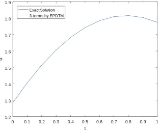
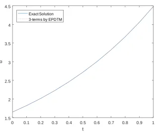
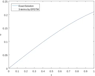
We present in this section to discuss our obtained results in comparison with their associated exact forms. Figures 1-2-3 are 2D plots of the ap-proximate solution and exact solution where x = y = 0:5 and t ₂ [0:1] for Example 1 and x = 0:5; t ₂ [0:1] for Examples 2-3. The tables 1-2-3 are Comparison of the absolute errors for the obtained results and the exact solution for Examples 1-2-3, where x; y; t₂[0:1]and n= 3.

We de…ne En(X; t) to be the absolute error between the exact solution

u(X; t) and n-term approximate solution by EPDTM

'_n(X; t) =

n 1 X

k=0

u(X; k)

as follows

(13)

0 0.1 0.2 0.3 0.4 0.5 0.6 0.7 0.8 0.9 1 t

1.2 1.3 1.4 1.5 1.6 1.7 1.8 1.9

u

Exact Solution 3-terms by EPDTM

Figure 1. The behavior of the exact solution and the 3-terms approximate solution for Example 1 whenx=y= 0:5.

Table 1. Comparison of the absolute errors for the obtained results and the exact solution for Example 1, where n=3

t=x; y 0:1 0:3 0:5 0:7

0:1 1.4226 10 9 1.5411 10 9 1.8085 10 9 2.2991 10 9

0:3 1.0648 10 6 1.1535 10 6 1.3536 10 6 1.7208 10 6

0:5 2.3382 10 5 2.5330 10 5 2.9725 10 5 3.7787 10 5

0:7 1.8000 10 4 1.9499 10 4 2.2882 10 4 2.9089 10 4

(14)

0 0.1 0.2 0.3 0.4 0.5 0.6 0.7 0.8 0.9 1 t

1.5 2 2.5 3 3.5 4 4.5

u

Figure 2. The behavior of the exact solution and the 3-terms approximate solution for Example 2 when x= 0:5.

Table 2. Comparison of the absolute errors for Example 2, where n=3

t=x; y 0:1 0:3 0:5 0:7

0:1 1.5572 10 9 1.9019 10 9 2.3230 10 9 2.8373 10 9

0:3 1.1688 10 6 _{1.4276 10} 6 _{1.7436 10} 6 _{2.1297 10} 6 0:5 2.5810 10 5 3.1525 10 5 3.8504 10 5 4.7029 10 5

0:7 2.0036 10 4 2.4472 10 4 2.9890 10 4 3.6507 10 4

(15)

0 0.1 0.2 0.3 0.4 0.5 0.6 0.7 0.8 0.9 1 t

0 0.05 0.1 0.15 0.2 0.25

u

Figure 3. The behavior of the exact solution and the 3-terms approximate solution for Example 3 when x= 0:5.

Table 3. Comparison of the absolute errors for Example 3, where n=3

t=x; y 0:1 0:3 0:5 0:7

0:1 1.9839 10 13 1.7855 10 12 4.9596 10 12 9.7209 10 12

0:3 4.3339 10 10 _{3.9005 10} 9 _{1.0835 10} 8 _{2.1236 10} 8 0:5 1.5447 10 8 1.3903 10 7 3.8618 10 7 7.5692 10 7

0:7 1.6229 10 7 1.4606 10 6 4.0574 10 6 7.9524 10 6

(16)

7. Conclusion

In this work, we used a mixed Elzaki transform and the projected dif-ferential transformation method, the advantage is providing an analytical approximation of the solution, usually an exact solution, in a fast conver-gent sequence for nonlinear wave-like equations with variable coe¢ cients. EPDTM can be performed very easily is more e¢ cient and reliable compared to the most known techniques (Adomian decomposition and homotopy per-turbation) as in [6], [7]. In addition, EPDTM is faster than ADM-HPM to solve this type of equation and can be applied to other nonlinear partial di¤erential equations.

References

[1] A. K. Alomari, M. S. M. Noorani, R. Nazar, Solutions of Heat-Like and Wave-Like Equations with Variable Coe¢ cients by Means of the Homotopy Analysis Method, Chinese Physics Letters, 25(2) (2008), 589.

[2] A. Atangana, E. Alabaraoye, Exact Solutions Fractional Heat-Like and Wave-Like Equations with Variable Coe¢ cients, Open Access Scienti…c Reports, http://dx.doi.org/10.4172/scienti…creports.633.

[3] A. Aslanov,Homotopy Perturbation Method for Solving Wave-Like Nonlinear Equa-tions with Initial-Boundary CondiEqua-tions, Discrete Dynamics in Nature and Society, Article ID 534165 (2011), 10 pages.

[4] T. M. Elzaki & S. M. Elzaki , Application of New Transform “Elzaki Transform” to Partial Di¤ erential Equations, Global Journal of Pure and Applied Mathematics, ISSN 0973-1768, Number 1 (2011), pp. 65-70.

[5] T. M. Elzaki and S. M. Elzaki and E. A. Elnour, On the New Integral Transform “Elzaki Transform” Fundamental Properties Investigations and Applications, Glo. J. Math. Sci., 4, (2012), 1-13.

[6] M. Ghoreishi, A.I.B. Ismail, N.H.M.Ali,Adomain decomposition method for nonlinear wave- like equation with variable coe¢ cients, Applied Mathematical Sciences, Vol. 4 ,No. 49, 2431- 2444, 2010.

[7] V.G. Gupta and S. Gupta,Homotopy perturbation transform method for solving non-linear wave- like equations of variable coe¢ cients, Journal of Information and Com-puting Science, Vol. 8, No.3,163-172, 2013.

[8] B. Jang,Solving linear and nonlinear initial value proplems by the projected di¤ eren-tial transform method. Computer Physics Communications 181, 848–854, (2010). [9] A. Kilicman and H. Eltayeb, A note on Integral transform and Partial Di¤ erential

Equation, Applied Mathematical Sciences, 4(3), (2010), PP.109-118. Mathematical Theory and Modeling, ISSN 2224-5804 (Paper), Vol.2, No.4, 2012.

[10] S. Momani, Analytical approximate solution for fractional heat-like and wave-like equations with variable coe¢ cients using the decomposition method, Applied Mathe-matics and Computation, 165 (2005), 459-472.

(17)

1 _{A. KHALOUTA, Laboratory of Fundamental and Numerical Mathematics,}

Departement of Mathematics, Faculty of Sciences. University of Sétif 1, 19000 Sétif, Algeria.

E-mail address: [email protected]

2 _{A. KADEM, Laboratory of Fundamental and Numerical Mathematics.,}

Departement of Mathematics, Faculty of Sciences. University of Sétif 1, 19000 Sétif, Algeria.