Modified Cat Swarm Optimization Algorithm for Design and Optimization of IIR BS Filter

Modified Cat Swarm Optimization Algorithm for

Design and Optimization of IIR BS Filter

Kamalpreet Kaur Dhaliwal, Jaspreet Singh Dhillon

Department of Electrical and Instrumentation Engineering, Sant Longowal Institute of Engineering and Technology,

Longowal, Sangrur, Punjab, India

Abstract— This paper proposes a solution methodology for the design of optimal and stable digital infinite impulse response (IIR) band stop (BS) filter by employing modified cat swarm optimization (CSO) algorithm. The error surface of digital IIR filters is non linear and multimodal because of the presence of the denominator terms. Therefore, the traditional filter design methods usually got stuck in the local minim. CSO is a novel population based global optimization technique which possesses global as well as local search capabilities. Here, the multicriterion optimization is used as the decisive factor that undertakes the minimization of magnitude approximation error and minimization of ripple magnitudes of pass band and stop band while satisfying the stability constraints that are imposed during the design process. For the intention of starting with an improved solution set, the opposition based learning strategy is incorporated in the conventional CSO. The developed algorithm is used to design the digital IIR band stop (BS) filter and attempts to find the optimal filter coefficients which are approximately close to the desired filter response. The computational results show that the proposed algorithm is capable of designing stable and optimal digital IIR BS filter structure that is better to the designs presented by other algorithms.

Keywords— Digital IIR filter, cat swarm optimization algorithm, opposition based learning, filter design, multiparameter optimization.

I. INTRODUCTION

The digital filters are generally of two types, finite impulse response (FIR) filters and infinite impulse response (IIR) filters. The digital FIR filter has a finite duration impulse response and its output depends upon the present and past input values only. Hence, these filters are known as non-recursive. On the other hand, the IIR filter has an infinite or continues impulse response and its output depend upon the present and past input values as well as on the previous output values. Hence, they are termed as recursive filters [1, 2]. Over the past few decades, the digital IIR filters have become the target of growing interest as they provide much better performance, improved selectivity and higher computational efficiency than their FIR counterparts for similar magnitude specifications. Also, they have a much sharper roll-offs in their frequency response than the FIR filters of equal complexity.

The digital IIR filter designing mainly follows two approaches: (i) transformation approach and (ii) optimization approach. The transformation approach involves the transformation of an analog filter to a digital filter for a given set of prescribed specifications [3]. But the

performance of digital IIR filters designed by using the transformation approach is not good as they require too much pre-knowledge and in most of the cases return a single solution. Also, the designing of digital IIR filter generally faces two problems that are (i) tendency of the filter to become unstable (ii) filter error surface is multimodal in nature due to which conventional design algorithms may stuck at local minima [4, 5]. The stability problem is handled by imposing stability constraints on the filter coefficients. In order to overcome the shortcomings of conventional methods and to achieve a global optimal solution, in the past years many nature inspired optimization algorithms have been implemented for the digital IIR filter design problem. Under the optimization approach various methods like the direct search and the gradient search methods have been proposed. Because of multimodal error surface, the conventional gradient-based algorithm easily stuck at local minima [6]. Therefore, in the past few years numerous nature inspired stochastic optimization technique like the hierarchal genetic algorithm (HGA) [7], hybrid taguchi genetic algorithm (HTGA) [8], taguchi immune algorithm (TIA) [9], real coded genetic algorithm (RCGA) [10], particle swarm optimization (PSO) [11], seeker optimization algorithm (SOA) [12], predator prey optimization (PPO) method [13], heuristic search method (HSM) [14] etc. have been developed and employed for optimal digital IIR filter designing. All these algorithms took the task of digital filter designing and strived hard to obtain structures that are stable and has optimized coefficients. Presently, the development of new and efficient optimization algorithms that use the magnitude approximation error and ripple magnitudes of both pass band and stop band as performance criteria for the designing of optimal digital IIR filters is very much in progress.

The remainder of this paper is organized as follows. Section 2 describes the digital IIR filter designing problem. The details of the mechanism for designing the digital IIR filter using cat swarm optimization algorithm and opposition based learning is described in section 3. Section 4 contains the proposed algorithm steps in detail. In section 5, the performance and statistical analysis of the proposed method has been carried out and the results obtained are compared with the design results in [7], [8], [9], [10] and [14]. Finally, section 6 contains the concluding remarks and scope for future work.

II. PROBLEM STATEMENT

The traditional design of digital IIR filter is generally realized by the following difference equation [1]:

 

 







 







   M 0 i N 1 k N k iu n i x y n k

x n

y (1)

where, M and N are the number of xi and xNk filter

coefficients, respectively, such that N ≥ M. u

 

n and y

 

n are its input and output, respectively. An equivalent transfer function of digital IIR filter is expressed as follows:

 

         N 1 k k k N M 0 i i i z x 1 z x z

H (2)

where, xi and xNk represent the values of the filter

coefficients,which produce the desired response.

Generally, the digital IIR filter is realized by cascading different first-order and second-order blocks together. The transfer function of the cascaded digital IIR filter is denoted byH



w,X



, where X indicates the filter coefficients. The magnitude of H



w,X



is denoted by H



w,X



. The basic

structure ofH



w,X



can be stated as [3]:





                                      N 1

k l 3 jw l 4 2jw jw 2 1 l jw l M 1

i 2i 1 jw jw i 1 e x e x 1 e x e x 1 e x 1 e x 1 x X , w H (3) where, N and M denotes the number of filter coefficients of the first and second order sections,l2M4



k1



2and

vector





T

D

x x x

X  _{1 2} denotes the filter coefficients

of dimension D×1, such that,D2M4N1.

In the IIR filter design process, the coefficients are optimized so that the approximation error function for magnitude is minimized. The magnitude response is specified at K equally spaced discrete frequency points in pass-band and stop-band. The absolute error is denoted by

 

X

e and is stated below:

 

 

 









K

0

k d k k

X , w H w H X e (4) where, H_d

 

w_k is the desired magnitude response of IIR

filter and is given as:

 

      stopband w for 0 passband w for 1 w H k k k d (5)

The ripple magnitudes of pass-band and stop-band are denoted by _p

 

x and _s

 

x , respectively and are given as:

 

X max_w



H



w_k,X





min_w



H



w_k,X





;w_k passband,

p  k  k 

 (6)

 

X max_w



H



w_k,X





;w_k stopband

s  k 

 (7)

The design of stable digital IIR filter requires the inclusion of stability constraints. Therefore, the stability constraints obtained by using the jury method [15] on the coefficients of the digital IIR filter stated in Eq. (9.1) - Eq. (9.5), are used in the optimization process. The multivariable constrained optimization problem is then stated as:

Minimize f(x) =e(x) (8) Subject to the stability constraints:

1+x2i+1≥ 0 (i=1, 2, …, N) (9.1)

1- x2i+1≥ 0 (i=1, 2, …, N) (9.2)

1-xl+3≥0 (l=2N+4(k-1)+2, k=1, 2, …, M) (9.3)

1+xl+2+xl+3≥0 (l=2N+4(k-1) +2, k=1, 2, …, M) (9.4)

1-xl+2+ xl+3≥0 (l=2N+4(k-1) +2, k=1, 2, …, N) (9.5)

Scalar objective constrained multivariable optimization problem is converted into scalar objective unconstrained multivariable optimization problem using exterior penalty function. Augmented objective function is defined as [16]:

    

x ex r Pterm



A   ₍₁₀₎ where,                N 1 k 2 M 1 i M 1 i 2 2

term 1 x2i 1 1 x2i 1 1 xl 3

P               N 1 k N 1 k 2 2 3 l 2 l 3 l 2

l x 1 x x

x

1 (11)

and r is a penalty term having a large value.

Bracket function for constraints given in Eqn. (9.1) and Eqn. (9.4) is stated below in Eqn. (12) and Eqn. (13) respectively:









              0 x 1 if , 0 0 x 1 if , x 1 x 1 1 i 2 1 i 2 1 i 2 1 i

2 (12)









                      0 x x 1 if , 0 0 x x 1 if , x x 1 x x 1 3 l 2 l 3 l 2 l 3 l 2 l 3 l 2

l (13)

Similarly, bracket functions for other constraints given by Eqn. (9.2), Eqn. (9.3) and Eqn. (9.5) are undertaken. Initial feasible solutions are generated applying constraint handling method [16], in which filter coefficients are randomly perturbed till the satisfaction of constraints. During the run the penalty terms are perturbed to zero by applying random constraint handling.

III.CAT SWARM OPTIMIZATION

A. Population Initialization

The initial step is to decide the number of individuals in the population i.e. the cats that will take part in the optimization process. Every individual/cat in the population has a position made up of D-dimensions, velocities for each dimension, a fitness value according to the fitness function and a seeking/tracing flag. The position of the cat represents the candidate solution and the fitness value of each cat represents the accommodation of the cat to the fitness function. The seeking/tracing flag is used to identify whether the cat is in seeking mode or tracing mode. The initial population of cats within the solution search space is initialized as follows:



x x





d 1,2,...,D;i 1,2,...,T



R

x

xidt _dmin _dmax _dmin  

(14)

And the velocity for each dimension is mathematically given as:



x v





d 1,2,...,D;i 1,2,...,T



R

v

v dmin

max d min d t

id     

(15)

where, represents the position and velocity of

the ith cat in dth dimension, respectively. And R is uniform random number between the range [0, 1]. The population may violate inequality constraints which are corrected by applying the random perturbation method.

B. Fitness Evaluation

The aim of the optimization process is to minimize the objective function. There is a possibility of the elements of parent/offspring to violate the constraint. Therefore, a penalty term is introduced and the objective function is penalized and changed to a generalized form which is mathematically expressed as follows:

 

X e

  

X R P



i 1,2,...,T



A_{i i}  _{i i}  _term  ₍₁₆₎

where, and penalty factor is given

by Eqn. (11). The value increases with the progress of the algorithm.

C. Oppositional Learning Strategy

The opposition based learning strategy helps CSO algorithm to take a start with some initial random solutions which are improved over time by moving towards an optimal solution. The computational time of any algorithm is an important parameter that is related to the remoteness of the initial guesses from the optimal solution. This can be improved by starting with a better solution by simultaneously checking the opposite solution in the search space. [19]. Therefore, starting with better guesses adjudged by its objective function has the ability to increase the convergence speed. The same approach is applied during the run, not only to initial solutions but also continuously to each solution in the current population to reach a final optimal solution. This can be mathematically expressed as:,



d 1,2,...,D;i 1,2,...,T



t

x x x

x_iT,d  _dl  _du  _id   (17)

where, l

d

x and x_duare lower and upper limits of filter coefficients, respectively and are expressed as follows:







       1 t ; T , , 2 , 1 i ; x min 1 t ; x x id min d l d

 (18)







       1 t ; T , , 2 , 1 i ; x max 1 t ; x x id max d u d  (19)

D. Seeking Mode

The mixture ratio (MR) is used to set the seeking/tracing flag, which decides the number of cats that would randomly be moved into the seeking mode and the tracing mode [20, 21]. The seeking mode corresponds to the global search procedure. This mode emulates the observant behaviour of cats by creating copies of the current solution. Each copy tries to improve the given solution through the exploitation process. After all copies have finished exploiting the current solution, that represent the new position on which the cat has to move, is selected. Seeking mode has four important parameters namely Memory Seeking Pool (MSP), Seeking Range of Dimension (SRD), Counts of Dimension to Change (CDC) and Self position consideration (SPC). For a cat, MSP is defined as the size of seeking memory for each cat indicating the points sought by each cat. SRD dictates the mutative ration for the selected dimensions. If a dimension is selected to mutate, the maximum difference between the new value and the old value cannot be out of the range defined by SRD. CDC indicates how many dimensions will be varied and SPS is a Boolean variable which decides whether the point on which the cat is already standing is a point, for one of the candidates to move to. The seeking mode involves the generation of t copies of the present position of ith cat, where t = MSP. If the value of SPC is true, let t = (MSP − 1), then retain the present position as one of the candidates. For each copy, according to CDC, randomly plus or minus SRD percents the present values and replace the old ones according to the following mathematical equations:



d 1,2,...,D;i 1,2,....,T



X cnvRS X

X_idc _id _{rd id}   ₍₂₀₎



d 1,2,...,D;i 1,2,....,T



X cnvRS X

X_idc _id _{rd id}   (21)

At the end of the seeking mode, the fitness of all copies is evaluated and from t copies the candidate with best fitness is selected and placed at the position of ith cat.

E. Tracing mode

The tracing mode corresponds to the local search technique where the rapid chase of the cat for its pray is mathematically modelled as a large change in its position. Then, the position and the velocity of ith cat in the D -dimensional space are mathematically expressed as follows:





T

iD 2 i 1 i

i x ,x ,...,x

X  and, (22)





T

iD 2 i 1 i

i v ,v ,...,v

V  (23) The global best position of the cat is represented

by Xg , where





T gD 2 g 1 g

g x ,x ,...,x

X  . In the tracing

mode the velocity and the position of the ith cat are updated using the following equations:



X X





d 1,2,...,D;i 1,2,...,T



CR wV

V id gd id

n

id      (24)



d 1,2,...,D;i 1,2,...,T



V X

where, w represents the inertia weight, C is the acceleration constant and R is a uniform random number distributed in the range [0, 1].

IV.DEVELOPED ALGORITHM AND DESIGN RESULTS The CSO algorithm with the opposition based learning technique is used to design the digital IIR BS filter. The

developed algorithm tries to have an optimal IIR BS filter structure while satisfying the stability constraints that are imposed during the design process. The procedure for implementation of CSO algorithm for digital IIR BS filter design is explained step by step as follows:

1. Initialize the algorithm parameters like number of cats i.e. the population size (NC), maximum iteration (ITMAX),

mixture ratio (MR), memory seeking pool (MSP), seeking range of dimension (SRD), counts of dimension to change

(CDC), self position consideration (SPC), C1, _xmax_{and x}min_.

2. Set t=0; generate an array of (D×T) size of uniform random numbers.

FOR d=1 to D

FOR i=1 to T

3. Randomly initialize the position of cats in D-dimensional space for the population, i.e. , using Eqn.

(14).

4. Randomly initialize the velocity for cats, i.e. , using Eqn. (15). 5. Compute the augmented objective function , using Eqn. (16). 6. Generate the initial population of individuals using opposition, Eqn. (17). 7. Compute the augmented objective function using Eqn. (16). 8. Compare and .

END FOR END FOR

9. Arrange Ai in ascending order and select first T cats out of 2T cats in the swarm.

10. Select best member with highest fitness out of T cats as and select the corresponding position as .

WHILE (T ) DO

11. Increment the iteration count, t=t+1. IF (seeking/tracing flag=1) THEN

12.Apply seeking mode steps given in Eqn. (20) and Eqn. (21). ELSE

13.Apply tracing mode steps given in Eqn. (24) and Eqn. (25). ENDIF

14. Select best member Abestand corresponding position as (Xid)best. 15. IF ( ) THEN

= ;

ENDIF ENDDO

For designing the digital IIR BP filter, 200 equally spaced points are set within the frequency domain [0, π]. For the purpose of comparison, the lowest order of the digital IIR BS filter is set exactly same as that set by Tang et al. [7] and Tsai et al. [8] i.e. the order is set equal to 4. The aim is to minimize the magnitude approximation error

and ripple magnitudes of both the pass-band and the stop-band, subject to the stability constraints given by Eqn. (9.1) - Eqn. (9.5) under the prescribed design conditions stated in Table 1. The control parameters used for CSO algorithm are given in Table 2. The final filter model obtained for the BS filter is given in Eqn. (26).

TABLE 1

PRESCRIBED DESIGN CONDITIONS FOR BS FILTER

Maximum value of H

 

w_i,x Pass band Stop band

1 0w0.25;0.75 w 0.4w0.6

TABLE 2

VALUES OF CONTROL PARAMETERS FOR BS FILTER

Parameter Number of cats

Mixture ratio

Maximum number of iterations

Memory seeking pool

Seeking range of dimension

Counts of dimension to

change

Notation NC XMR ITMAX MSP SRD CDC

 









z 0.676532z 0.538100



z 0.794511z 0.521102



000348 . 1 z 404512 . 0 z 003495 . 1 z 357345 . 0 z 364876 . 0 H

2 2

2 2

z BS

 

 

 

 



(26)

The results of the developed algorithm for designing the BS filter are summarized in Table 3, where the comparison of the obtained results is carried out with the design results given by other methods like HGA[7], HTGA [8], TIA [9], RCGA [10] and HSM [14]. From the table is can be observed that the developed algorithm is capable of

obtaining a lower value of magnitude response error than the other algorithms. In terms of pass band and stop band performance, the proposed algorithm produced results that are superior or atleast comparable to the other well established algorithms.

TABLE 3

DESIGN RESULTS FOR BS FILTER

Method Magnitude Error Filter

order Pass band performance Stop band performance

Opposition aided CSO 3.5744 4 0.9633_(0.0387) ≤|H(e)|≤1.0020 |H(e)|_(0.1036) ≤0.1036

RCGA[10] 3.7976 4 0.9774_(0.0415) ≤|H(e)|≤1.0190 |H(e)|_(0.1164) ≤0.1164

HSM [14] 3.7699 4 0.9652_(0.0434) ≤|H(e)|≤1.0080 |H(e)|_(0.1060) ≤0.1060

TIA[9] 4.1275 4 0.9560_(0.0440) ≤|H(e)|≤1.0000 |H(e)|_(0.1164) ≤0.1164

HTGA[8] 4.5504 4 0.9563_(0.0437) ≤|H(e)|≤1.0000 |H(e)|_(0.1013) ≤0.1013

HGA[7] 6.6072 4 0.8920_(0.1080) ≤|H(e)|≤1.0000 |H(e)|_(0.1726) ≤0.1726

The frequency response and pole-zero plots of the designed optimal digital IIR BS filter are represented in Fig. 1 and Fig. 2, respectively. The frequency response plot depicts that the designed BS filter strictly follows the constraints that are imposed during its design process. Also, in the pole-zero plot, all the poles lie inside the unit circle, which proves the stability of the designed BS filter.

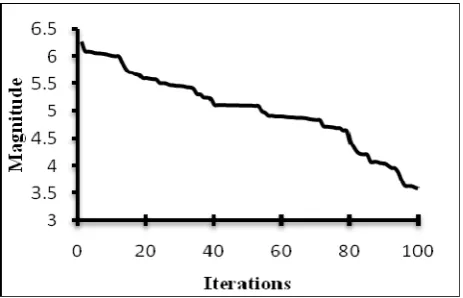
Also, the magnitude versus iterations graph (Fig. 3) shows the effectiveness of the proposed algorithm. It is clear from the figure that the magnitude response error decreases with the number of iterations and reach a minimum or optimum value at the 100th iteration.

0 0.1 0.2 0.3 0.4 0.5 0.6 0.7 0.8 0.9 1

0 0.1 0.2 0.3 0.4 0.5 0.6 0.7 0.8 0.9 1

M

a

gn

it

ud

e

Normalized frequency Band stop Filter

-1 -0.5 0 0.5 1

-1 -0.5 0 0.5 1

Real part

Im

agi

n

ar

y

par

t

Band Stop Filter

Fig. 3: Magnitude versus Iterations for BS filter

V.ROBUSTNESS AND STATISTICAL ANALYSIS Robustness is used to evaluate the performance of an evolutionary algorithm. The CSO algorithm starts with random initialization of the population of cats, which makes randomness an inherent element of CSO. Therefore, the robustness of CSO algorithm to achieve global optimum design solution for order 4 BS filter is determined by having 100 independent trial runs with random seed numbers. The variations in the value of overall objective function have been observed and the maximum value, minimum value, average value and standard deviation in the value is calculated and given in Table 4. From Table 4, it can be observed that in each case the value of standard deviation is very small which indicates that the developed algorithm has outstandingly strong robustness. To further validate the obtained results and

to confirm the effectiveness of the developed algorithm for digital IIR BP filter design, a non-parametric statistical test called the Wilcoxon’s signed rank test for single sample is used. This test is conducted on the results obtained by the developed algorithm for the BS filter with a significant

level of by comparing them with the results

provided by other existing algorithms. Firstly, the sum of positive ranks (R+) and the sum of negative ranks (R-) is calculated and then the p-value is determined in each case. The Wilcoxon’s signed rank test (Table 5) depicts that the results of the developed algorithm are significantly better then the HGA, HTGA, TIA, RCGA, and HSM algorithms as the p-value is less than 0.10 in all the cases and facilitates the designing of not only stable but optimal digital IIR BS filter.

TABLE 4

MAXIMUM, MINIMUM, AVERAGE AND STANDARD DEVIATION OF MAGNITUDE ERRORFOR BS FILTER

Order Maximum

magnitude Error

Minimum magnitude Error

Average magnitude Error

Standard Deviation of magnitude Error

4 6.2654 3.4959 4.0443 0.0229

TABLE 5

STATISTICAL ANALYSIS RESULTS BASED ON WILCOXON’S SIGNED RANK TEST FOR LOWER ORDER BS FILTER

Performance p-value

Magnitude approximation error 0.10 0 10 0.033945

Pass-band performance 0.10 0 10 0.033945

Stop-band performance 0.10 0 10 0.033945

VI.CONCLUSION

In this paper, the CSO algorithm together with the opposition based learning strategy is used to design the optimal and stable digital IIR BS filter. CSO possesses qualities like robustness and local as well global search abilities and thus is capable of returning a global optimal solution which is not possible in some conventional optimization algorithms. The proposed approach is executed to solve the multi criterion optimization problem of designing digital IIR BS filter. The experimental results show that the results obtained by CSO algorithm in terms of

REFERENCES

[1] Proakis, J. G. and Manolakis D. G., “Digital Signal Processing: Principles, Algorithms and Applications,” New Delhi: Pearson Education, Inc., 2007.

[2] Ifeachor, E. C. and Jervis, B. W., “Digital Signal Processing: A Practical Approach,” 2nd edition, Pearson Education, Singapore, 2003.

[3] Mitra, S. K. and Kaiser, J. F., “Handbook for Digital Signal Processing,” Wiley, New York, 1993.

[4] Li, J. H. and Yin, F. L., “Genetic Optimization Algorithm for Designing IIR Digital Filters,” Journal of China Institute of Communications China, Vol. 17, pp. 1–7, 1996.

[5] Lu, W. -S. and Antoniou, A., “Design of Digital Filters and Filter Banks by Optimization: A State of the Art Review,” in: Proceeding of European Signal Processing Conference, Finland, 2000.

[6] Panda, G., Pradhan, P. M. and Majhi, B., “IIR System Identification Using Cat Swarm Optimization,” Expert Systems with Applications, Vol. 38, pp. 12671-12683, 2011.

[7] Tang, K. S., Man, K. F., Kwong, S. and Liu, Z. F., “Design and Optimization of IIR Filter Structure using Hierarchical Genetic Algorithms,” IEEE Transaction on Industrial Electronics, Vol. 45, pp. 481–487, 1998.

[8] Tsai, J. -T., Chou, J. -H. and Liu, T.-K., “Optimal Design of Digital IIR Filters by using Hybrid Taguchi Genetic Algorithm,” IEEE Transactions on Industrial Electronics, Vol. 53, pp. 867– 879, 2006.

[9] Tsai, J. -T. and Chou, J. -H., “Optimal Design of Digital IIR Filters using an Improved Immune Algorithm,” IEEE Transactions on Signal Processing, Vol. 54, pp. 4582–4596, 2006. [10] Kaur, R, Patterh, M. S, Dhillon, J. S., “Real Coded Genetic

Algorithm for Design of IIR Digital Filter with Conflicting Objectives,” International Journal of Applied Mathematics and Information Sciences, Vol. 8, pp. 2635-2644, 2014.

[11] Chaohua, D., Chen, W. and Zhu, Y., “Novel Particle Swarm Optimization for Low Pass FIR Filter Design,” WSEAS Transactions on Signal Processing, Vol. 8, pp. 111-120, 2012. [12] Chaohua, D., Chen, W. and Zhu, Y., “Seeker Optimization

Algorithm for Digital IIR Filter Design,” IEEE Transactions on Industrial Electronics, Vol. 57, pp. 1710-1718, 2010.

[13] Singh, B., Dhillon, J. S., Brar, Y. S., “Predator Prey Optimization Method for the Design of IIR Filter,” WSEAS Transactions on Signal Processing, Vol. 9, 2013, pp. 51-62.

[14] Kaur, R., Patterh, M. S., Dhillon J. S. and Singh, D., “Heuristic Search Method for the Design of IIR filter,” WSEAS Transactions on Signal Processing, Vol. 8, pp. 121-134, 2012.

[15] Jury, I., “Theory and Application of the Z-Transform Method,” New York: Wiley, 1964.

[16] Jiang, A. and Kwan, H. K., “IIR Digital Filter Design with New Stability Constraint based on Argument Principle,” IEEE Transactions on Circuit and Systems-I, Vol. 56, pp. 583–593, 2009.

[17] Tsai, P. -W., Pan, J. -S., Chen, S. -M. and Lio, B. –Y., “Enhanced Parallel Cat Swarm Optimization based on the Taguchi method,” Expert Systems with Applications, Vol. 39, pp. 6309-6319, 2012. [18] Mohan, P. M. and Panda, G., “Solving Multi-objective Problems

using Cat Swarm Optimization,” Expert Systems with Applications, Vol. 39, pp. 2956-2964, 2012.

[19] Rahnamayan, H. R., Tizhoosh and Salama, M. A., “Opposition based Differential Evolution,” IEEE Transactions on Evolutionary Computations, Vol. 12, pp 64-79, 2008.

[20] Chu, S. C. and Tsai, P. W., “Computational Intelligence based on the Behavior of Cat,” International Journal of Innovative computing, Information and Control, Vol. 3, pp.163-173, 2007.