Sparse and Low-Rank Modeling on High Dimensional Data: A Geometric Perspective.

(1)

ABSTRACT

BIAN, XIAO. Sparse and Low-Rank Modeling on High Dimensional Data: A Geometric Perspective. (Under the direction of Dr. Hamid Krim.)

High dimensional data exhibits distinct properties compared to its low dimensional counterpart, which causes a common performance decrease and a formidable computa-tional cost increase of tradicomputa-tional approaches. Novel methodologies are therefore needed to characterize data in high dimensional spaces. In this thesis, we study the representa-tion of high dimensional data by different low dimensional structures embedded in high dimensional spaces, and focus on novel paradigms for general machine learning purpose, such as clustering, classification and inference.

To address the nonlinearity of imagery sequential data, we map images into a circulant operator space with a proper Riemannian metric associated to data samples. A low rank model to achieve the optimal circulant operator subspace for the given dataset is proposed with an efficient algorithm on video-based human activity classification.

In order to further characterize general high dimensional data, we study the union-of-subspaces (UoS) model, as a generalization of the subspace model. The UoS model maintains the simplicity of the subspace model, and additionally has the ability to ad-dress nonlinear data. We show a sufficient condition to use l1 minimization to reveal the underlying UoS structure, and propose a bi-sparsity model to recovery data from errors/corruptions. An effective algorithm, robust subspace recovery via bi-sparsity pur-suit, is proposed and applied to data recovery and clustering.

(2)

(3)

c

(4)

Sparse and Low-Rank Modeling on High Dimensional Data: A Geometric Perspective

by Xiao Bian

A dissertation submitted to the Graduate Faculty of North Carolina State University

in partial fulfillment of the requirements for the Degree of

Doctor of Philosophy

Electrical Engineering

Raleigh, North Carolina 2014

APPROVED BY:

Dr. Huaiyu Dai

Dr. Edgar Lobaton

Dr. Larry K. Norris

(5)

DEDICATION

(6)

BIOGRAPHY

Xiao Bian received his B.E. degree (2008) in Tsinghua University, Beijing and the M.Sc (2011) degree in Electrical Engineering in North Carolina State University, Raleigh, North Carolina. In 2009, he joined the Vision, Information and Statistical Signal Theories and Applications group (VISSTA) under the direction of Dr. Hamid Krim and became a PhD student since 2010.

(7)

ACKNOWLEDGEMENTS

Everyone is shaped by their culture, their environment, and especially by the people around. By all means, I cannot emphasize enough the importance of the people I met to me, to this work, during my PhD study. This piece of work is not just about my research, but also a tip of iceberg that how much help and guidance I have received during these years.

I would like to first thank my advisor Dr. Hamid Krim for his instruction and ac-company on my journey in high dimensional spaces. He has guided me through my exploration using his extraordinarily broad knowledge and sharp intuition in different areas, such as mathematics, signal processing, machine learning, computer vision, etc. Moreover, his great patience and trust on students has no doubt encouraged me to over-come difficult problems, and has created a very active and healthy research atmosphere in VISSTA group.

I would also like to thank my other committee members, in alphabetical order, Dr. Huaiyu Dai, Dr. Liyi Dai, Dr. Edgar Lobaton and Dr. Larry Norris, for their invaluable advice and help during my PhD study. I have been extremely fortunate to have such a diversified committee, from engineering to mathematics, to guide me through any potential problems. Moreover, I want to especially acknowledge Dr. Alex Bronstein for all the fascinating discussions, which help me formulate some of the ideas of my research work.

Additionally, I want to express my gratitude to all my lab mates, for the time shared with them, for their support and all helpful discussions.

(8)

(9)

LIST OF TABLES

(14)

LIST OF FIGURES

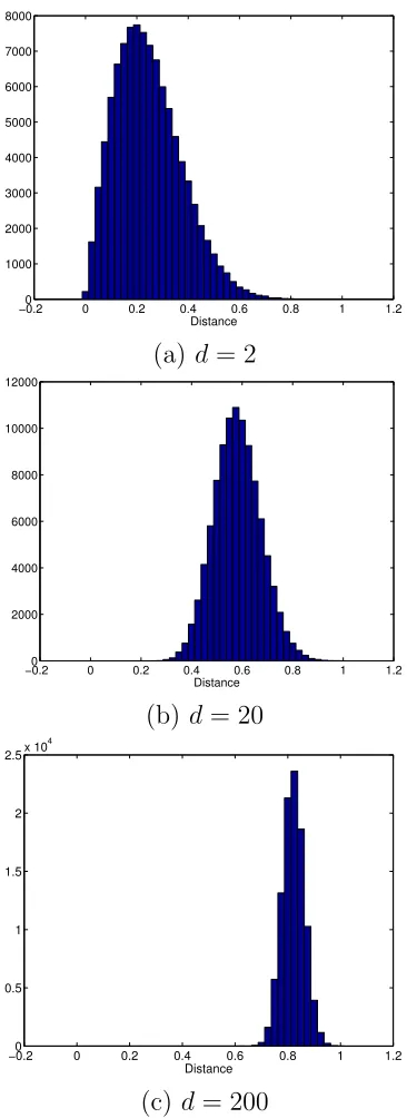
Figure 2.1 Euclidean distance become indiscernible in a high dimensional space 5 Figure 2.2 The histogram of Euclidean distances in different dimensions between

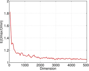
random points under Gaussian distribution . . . 7 Figure 2.3 E{dmax/dmin} vs Dimensions . . . 8

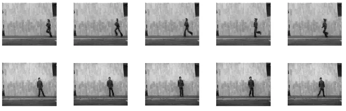
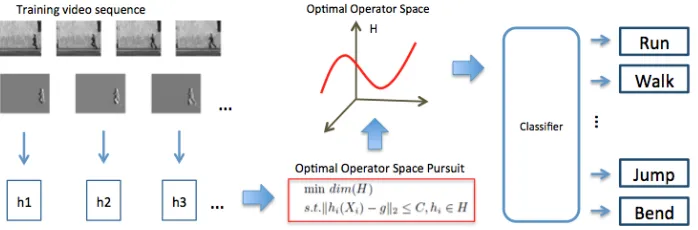
Figure 3.1 Graph of nonlinear function g(α, β) compared to a 2-D gaussian . . . 18 Figure 3.2 Sample frames of human activity video clips (Upper: running; Lower:

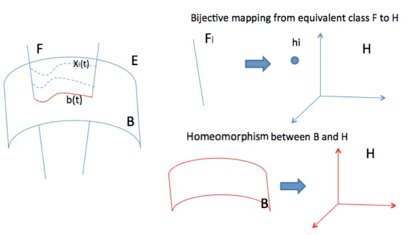
Siding) . . . 22 Figure 3.3 Fiber bundle structure for data space . . . 23 Figure 3.4 Homeomorphism between H and B . . . 25 Figure 3.5 Examples human activity video sequence and difference images.(The

upper case is running, and the lower case is walking) . . . 29 Figure 3.6 Optimal operator space intends to obtain a more compact

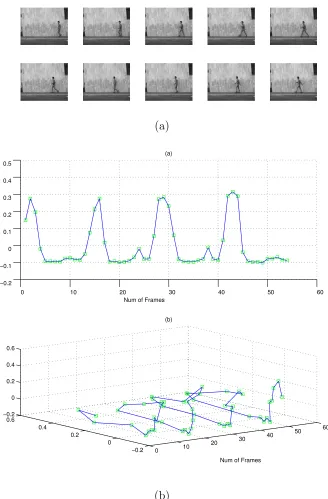
representa-tion for each sample video sequence, upon which a classifier is built. . . . 31 Figure 3.7 Classification rate vs percentage of data using as training set . . . . 32 Figure 3.8 (a) A sample walking sequence (b) The walking sequence embedded

in 1D and 2D (c) A sample bending sequence (d) Bending sequence embedded in 1D and 2D (x-axis is the index of frames) . . . 35 Figure 3.9 (a) A sample bending sequence (b) Bending sequence embedded in

(15)

Figure 3.10 (a) Embedded sequence of walking. Left: before correction. Right: after correction. (b)Embedding sequence of bending. Left: before

correction. Right: after correction. . . 38

Figure 3.11 (a) Embedded sequence of walking. (b) Project another sequence of walking into the same space (c)Project a sequence of bending into the same space . . . 40

Figure 3.12 Classfication rate compared to results without using continuous HMM. (Red: with continuous HMM. Blue: without continuous HMM) . . . 44

Figure 4.1 Data in a union of subspaces . . . 47

Figure 5.1 Illustration of Problem 5.1.1 . . . 61

Figure 5.2 An example of robust subspace exact recovery. . . 68

Figure 5.3 Comparison with Robust PCA. . . 69

Figure 5.4 Overall recovery results of RoSuRe and Robust PCA. [0 0.2] is mapped to [1 0] of grayscale image . . . 71

Figure 5.5 Background subtraction on traffic videos (static camera) . . . 72

Figure 5.6 Background subtraction on traffic videos (panning camera) . . . 73

Figure 5.7 Coefficient matrixW (a) without rearrangement according to the po-sition of the camera (b) with rearrangement according to the popo-sition of the camera . . . 74

Figure 5.8 Sample face images in Extended Yale face database B . . . 74

Figure 5.9 Clustering Accuracy vs The value of λ . . . 75

Figure 5.10 Affinity matrix for face images from different subjects . . . 76

Figure 5.11 Recovery results of human face images. The three rows from top to bottom are original images, the components E, and the recovered images, respectively. . . 77

Figure 6.1 An example of the result of SNS-BP . . . 87

Figure 6.2 kNˆk0/kNk0 vs Sparsity . . . 88

Figure 6.3 Sample synthetic data matrix and its underlying structure . . . 89

(16)

(17)

Chapter 1 Introduction

High dimensional data analysis has recently become a central topic in both academia and industry. The fast progress of techniques related to data acquiring, storage and processing has lead the researchers, from applied mathematicians to electrical engineers, to face problems of data of increasing size and dimensions.

Many well-established problems, such as data classification and clustering, therefore encounter novel challenges in the context of high dimensionality. Generally, the increas-ing dimensionality comes with redundant and irrelevant information, which may actually hinder the discovery of key information without carefully designed methods. The combi-natorial nature of finding the suitable features essentially makes the problem of feature selection even more challenging with high dimensional data. Additionally, insufficient samples in the vast high dimensional space make the probabilistic estimation unreliable. Furthermore, the distinct properties of high dimensional space, such as discernible Eu-clidean distance [2] and “the hubness” [82], also impact the performance of traditional data analysis algorithms on high dimensional data.

(18)

1.1 Outline

The rest of the thesis is organized as follows. In Chapter 2, we first give a review of the research on the properties of high dimensional spaces, and the state-of-the-art on the high dimensional data models. In fact, these works shed light on our framework of high dimensional data analysis.

In Chapter 3, we propose a low dimensional model, an optimal circulant operator subspace, to analyze imagery data. Natural images exhibit high nonlinearity, which usually causes the failure of linear low dimensional models in finding a low dimensional embedding. Instead of directly working on the high curvature unknown image space, we utilize the circulant operator space, with a properly defined Riemannian metric based on given image samples, to find an appropriate low dimensional embedding of the given image set. To further analyze the sequential imagery data, we exploit a fibre bundle formalism to model various realizations of each trajectory, and characterize these high dimensional data sequences by an optimal operator space. The low dimensional structure intrinsic to the data is further explored, by minimizing the dimension of the operator subspace under data-driven constraints.

In light of the parsimonious degrees of freedom of real-world data, we introduce a more advanced model, the union of subspaces (UoS), to characterize high dimensional data in Chapter 4. As a generalization of the subspace model, this model preserves the simplicity of the subspace model, and approximate the nonlinearity of the data distribu-tion using a union of subspaces. We demonstrate the formuladistribu-tion of the UoS model as a l1 minimization problem, and show a sufficient condition for the minimizer to reveal the underlying UoS structure of the given dataset. We further discuss the state-of-the-art algorithms to solve this problem.

(19)

the effectiveness of our method by experiments on both synthetic data and real-world vision data, and illustrate the potential applications on data recovery and data clustering problem.

Towards the discovery of latent variables, we study sparse models in dictionary learn-ing in Chapter 6, and relate this problem with another interestlearn-ing topic, sparse null space problem (SNS). We investigate the relation between the SNS problem and the analysis dictionary learning problem, and show that the SNS problem plays a central role, and may be utilized to solve dictionary learning problems. Moreover, we propose an efficient algorithm of sparse null space basis pursuit, and extend it to a solution of analysis dic-tionary learning. Experimental results on numerical synthetic data and real-world data are further presented to validate the performance of our method.

Finally, in Chapter 7, we conclude our journey in high dimensional spaces with sparsely distributed, structured data.

1.2 Notation

A brief summary of notations used throughout this thesis is follows: The dimension of a m×n matrix X is denoted as dim(X) = (m, n). kXk0 denotes the number of nonzero elements in X, while kXk1 denotes the vector l1 norm. For a matrix X and an index set J, we let XJ be the submatrix containing only the columns of indices in J. col(X)

denotes the column space of matrix X. We write PΩAX as the orthogonal projection of

matrix Xon the support of A, andPΩc

AX =X−PΩAX. The sparsity of a m×n matrix X is denoted byρ(X) = kXk0

(20)

Chapter 2 Review of Previous Research

2.1 The Curse of Dimensionality

The term “the curse of dimensionality” was first proposed by Richard Bellman in the con-text of dynamic programming [11]. With more and more exposure to high dimensional data in both academia and industry, it has been widely used to represent the challenges of high dimensional data analysis. In this section, we provide a brief review of recent and current research on exploring the properties of high dimensional space. Indeed, these distinct properties of high dimensional space unveil the reason why popular algorithms like k-nearest neighbors (KNN) fail, and further shed light on possible approaches on high dimensional data analysis.

One obvious yet important property of high dimensional space is the insufficiency of data samples. In particular, the volume among samples goes exponentially with the di-mensionality, which essentially implies that, to maintain the same level of sample density, we also need the sample size to increase exponentially. Take images/videos for instance, each data point has typically tens of thousands dimension. It is hence very difficult to estimate the data distribution in a high dimensional space, with a limited number of samples [16].

(21)

Figure 2.1: Euclidean distance become indiscernible in a high dimensional space

also introduce more noise components to the data [107]. Additionally, the number of irrelevant features also increases in a higher dimensional feature space. In fact, in most real-world problems, an effective data model is usually dominated by only a few variables. It would rather lead to ambiguity with many more features than the intrinsic degrees of freedom of a model. Considering human activity classification for example, the pixels of background and those of a person’s clothes are typically not related to the class identity of each presented image. It is hence unwise to treat each pixel as one feature and to address the activity classification problem in this high dimensional feature space, since the same activities may show in completly different backgrounds and contexts [16].

Furthermore, the Euclidean distance in high dimensional spaces becomes indiscernible [51] [2], which essentially shakes the foundation of KNN-based approaches on high di-mensional data.

Specifically, [51] shows that, assume the data distribution in all dimensions are i.i.d and all the appropriate moments are finite, then for every >0, the maximum distance dmax and the minimum distance dmin ofN points to the query point satisfy the following

relation,

lim

(22)

Since a lot of distances are similar, a small perturbation may lead to an entirely different nearest neighbor.

In Fig. 2.2, we show the distribution of pair-wise distances of randomly generated points in different dimensions. In particular, the data distribution in each dimension is i.i.d Gaussian. To better visualize the results, we further normalize the distance such that the maximal distance in each case is 1. We can see the trend that, from d = 2 to d = 200, the distribution of distance becomes increasingly concentrated and inclines to 1. In the 200 dimensional space, all pair-wise distance become similar to each other and close to the maximum.

We further show the mean ratio of dmax to dmin in spaces with various dimensions

in Fig. 2.3. We use the same method to generate data as in Fig. 2.2. When the dimensionality of the space increases, the ratio ofdmax todmin is getting closer to 1. All

these numerical results illustrate that the maximum distance and minimum distance of a dataset become indiscernible in high dimensional spaces. These phenomena essentially imply the instability of kNN-based approaches in high dimensional spaces.

2.2 Low Dimensional Structures in High Dimensional

Spaces

A natural approach to high dimensional data analysis is dimension reduction. If we can indeed find a more compact space of the given data, then the original challenging high dimensional problem would degenerate to its low dimensional counterpart. Extensive research has been carried out to model and to analyze the distribution of a given dataset as some low dimensional structure embedded in a high dimensional space [85] [35] [96]. Yet ahead of reviewing the algorithms of dimension reduction, it is of fundamental interest to validate the existence of such low dimensional structures in high dimensional data.

(23)

−0.20 0 0.2 0.4 0.6 0.8 1 1.2 1000

2000 3000 4000 5000 6000 7000 8000

Distance

(a) d= 2

−0.20 0 0.2 0.4 0.6 0.8 1 1.2

2000 4000 6000 8000 10000 12000

Distance

(b) d= 20

−0.20 0 0.2 0.4 0.6 0.8 1 1.2

0.5 1 1.5 2 2.5x 10

4

Distance

(c) d= 200

(24)

0 1000

2000

3000

4000

5000

1

1.2

1.4

1.6

1.8

2 Dimension

E{Dmax/Dmin}

(25)

pairwise distance between these points preserved as

(1−)kx−yk2 ≤ kf(x)−f(y)k2 ≤(1 +)kx−yk2,∀x,y∈S. (2.2)

Given a high dimensional dataset, especially when the dimensionality is larger than the number of data points, JL lemma guarantees that we can always find a linear mapping to map the high dimensional data into a low dimensional space, without much loss of information.

Furthermore, from a practical perspective, extensive works on different dataset show that low dimensional structures exist ubiquitously in real-world datasets, such as human faces, natural images and video sequences [96] [35] [85] [25]. Indeed, the degrees of freedom of a real-world dataset is typically much lower than the ambient space dimension. The challenge, therefore, is to recovery the underlying low dimensional structure in a given high dimensional dataset.

In particular, when the data is concentrated in a subspace, and is contaminated by mild noise, principal component analysis (PCA) is introduced to find the optimal subspace for the dataset [76] [37]. PCA essentially finds the directions that maximize the variance of a given dataset. The distribution of the data is therefore preserved in a low dimensional space to a maximum extent. Equivalently, we can also formulate this problem as an constrained optimization problem as follows,

min

Y kX−YkF s.t. rank(X)≤k, (2.3)

where X is the data matrix, and Y is the corresponding low dimensional embedding. Note that (2.3) has a closed-form solution, by keeping the topksingular values and their associated singular vectors of X [37].

However, PCA is not robust to outliers, and often fails to recover the intrinsic low dimensional structure with the presence of outliers. To further solve this issue, robust PCA was proposed to recover the low dimensional structure with the presence of er-rors/outliers [25]. Specifically, given a dataset X = [x1,· · · ,xn], xi ∈ Rn, the goal is

(26)

decom-position can be done by simultaneously minimizing the nuclear norm of L, which can be seen as a convex relaxation of the rank of L [22], and the l1-norm of E, which is the convex relaxation of the sparsity of E [65],

min

L,E kLk∗+λkEk1 s.t. X=L+E. (2.4)

This model can recover the low dimensional subspace for a given dataset more accurately with the presence of outliers and sparse errors [25].

Besides the subspace model, data may exhibit nonlinear relations among themselves, and are therefore distributed in a manifold embedded in a high dimensional space from a more general perspective. Imagine the points distributed in a 2-sphere S2 _embedded inR3_{. Finding an optimal subspace for this dataset, which is essentially}_R3 _{in this case,} will make us lose insight of the degree of freedom being actually 2. Various manifold learning algorithms are proposed to learn the underlying data manifold embedded in high dimensional spaces [85] [9] [35] [95]. One effective way is to preserve the geodesic distance instead of Euclidean distance in the original high dimensional space, upon which the algorithm Isomap is built [95]. Specifically, a graph based on k nearest neighbors is constructed. Isomap then pursues a low dimensional embedding by preserving the pairwise geodesic distances on that graph. The resulting low dimensional embedding reflects more of the intrinsic geometry of the given data compared to linear embeddings as the subspace model. Yet one potential problem for Isomap is that, miss-calculated k nearest neighbors can cause a dramatical change on geodesic distances, the so called “short-circuit errors” [5]. The whole embedding may change, as a result.

In contrast to Isomap that emphasizes longer distances more than the shorter ones, another way to preserve the intrinsic geometry of high dimensional data, named locally linear embedding (LLE), is to focus on shorter distances. Specifically, LLE utilizes k nearest neighbors to estimate the tangent space of each point, and preserves the local neighborhood relations in each tangent plane in the low dimensional embedding space. Instead of preserving geodesic distances, LLE are more robust to “short-circuit errors” by concentrating on local neighborhoods.

(27)

preserv-ing some properties of this graph in the low dimensional embeddpreserv-ing space. Essentially, this weighted neighborhood graph is considered to be an approximation of the low di-mensional data manifold. It is therefore natural to consider approaches that preserves the graph structure rather than only distances. Laplacian eigenmaps is one of the repre-sentative state-of-the-art in this category [9]. This algorithm reconstruct the graph in the low dimensional embedding space by preserving the corresponding Laplacian operator. Laplacian eigenmaps focus on intrinsic geometric structures, and is hence insensitive to noise [9].

As we discussed above, manifold learning algorithms rely on the approximation of the tangent space of the data manifold using k nearest neighbors. When the k nearest neighbors become unreliable, or the local sample density is not sufficient to estimate the tangent space, then the accuracy of the low dimensional embedding degrades dramati-cally. Unfortunately, these are the typical issues we are facing in high dimensional data analysis [39] [51] [82]. Without knowing reliable relations among data samples, embed-ding data into a low dimensional space still suffers from “the curse of dimensionality” from the beginning. Recent research on sparse representation shows that we can utilize the property of high dimensional data to conquer them [42] [34] [44] [101].

The story of sparse models starts from the notion that the number of degrees of freedom of high dimensional data is much smaller than the dimensionality of the ambient space [42]. In fact, consider the model behind a given high dimensional data sample, the underlying dominant variables are typically very few, and hence can be represented in a low dimensional space. Specifically, assume that each data sample is a linear combination of k atoms from an atom set or dictionaryD, we then have

x= X

di∈D

widi, i= 1,· · · , k. (2.5)

To formulate this problem into a matrix form, (2.5) is then written as

x=Dw,kwk0 ≤k. (2.6)

(28)

seems fail to escape from “the curse of dimensionality”. However, recent research shows that we can efficiently find w, when D approximately preserves the length of sparse vectors, by considering the convex relaxation of (2.6) [42] [23], and thereby solving the following optimization problem,

min

w kwk1 s.t. Dw=x. (2.7)

We can then use a k-sparsity vector w to represent each x. Consider data samples that share the same set of underlying variables and reside in the same subspace, we therefore have a union of subspaces (UoS) for different subsets of data that are dominant and represented by different subsets of variables. The UoS model can be seen as a general-ization of the subspace model, but is able to address the nonlinear data distribution of different topologies. In particular, the data samples in the same subspace preserve the local linearity. However, data from different subspaces exhibit highly nonlinear relations. The addition of two points from different subspaces is not able to produce any valid data. The vast volume among the union of subspaces coincides with the fact that real-world data only reside in a tiny fraction of the high dimensional ambient space. Moreover, the UoS model relies less on the local relations of each data, and is hence insensitive to different topologies of data distributions [93] compared to kNN-based manifold learning algorithms [5].

Research has also explored the UoS structure of a high dimensional dataset when a well-formulated dictionary is not available [44] [68] [93]. Specifically, the data matrix X

is utilized as a dictionary D, and the problem of (2.6) is formulated as follows,

min

W kWk1 s.t. XW=X, diag(W) = 0. (2.8)

(29)

in the data matrix, and the problem is formulated as

min

W,EkWk∗+λkEk1 s.t. X =XW+E. (2.9)

(30)

Chapter 3 An Optimal Circulant Operator

Subspace: Mending Nonlinearity

3.1 Introduction

One of the major challenges of high dimensional data analysis is that, nonlinearity often accompanies high dimensionality. The high dimensionality, representing the context of the problem, becomes even more puzzling when the curved data manifold exploits the vast space of a high dimensional world. In particular, when the data reside in a manifold embedded in a Euclidean space, traditional dimension reduction techniques, such as PCA, can only find the minimum subspace that contains the data manifold. Therefore, if the data manifold itself is highly curved, i.e. of high curvatures, pursuing a linear subspace just provides a very coarse measure of the data space.

(31)

do any interpolation.

The first step to analyzing a large high dimensional dataset therefore always in-volves addressing the nonlinearity. On one hand, we can directly learn the data mani-fold from the given samples, and therefore have a nonlinear dimension reduction on the dataset [18] [1] [35] [10] [104]. This approach utilizes the relations among various im-ages to estimate the underlying manifold structure. It, however, requires dense samples to cover the high curvature area, which is extremely difficult to satisfy when the data dimension is high. On the other hand, we can mitigate the nonlinearity of the data by extracting appropriate features by exploring the structures inside each sample [48]. Yet it is difficult and rather heuristic to design feature extractors that are adaptive to a specific dataset. Moreover, the lack of a framework of feature extractor design impacts the gen-eralizability of this class of method. The problems of these existing methods naturally raise a question about the integration of these two classes of approaches, i.e. is there a general framework for feature extraction to mitigate the nonlinearity, or equivalently mapping the given data to another space, and further learn the manifold structure in the feature space? If so, would it provide us a more accurate description of the given high dimensional data?

(32)

explicitly characterize the temporal relations among frames. We illustrate the viability of the framework and validate the models by human activity video sequence data analysis.

3.2 Background

Of keen interest to artificial intelligence and computer vision, research activity in video sequence data analysis has witnessed an explosive growth in recent years. Tools from areas, such as machine learning, computer vision, optimization and statistical analysis have been collectively utilized to address this problem [59] [78] [61] [99] [18] [1] [104].

In constrast to classical low dimensional signal processing, where random noise is the major challenge, the key factor in video sequence analysis is the discovery of useful information hidden in high dimensional data. More specifically, natural images are widely recognized to reside in a low dimensional space given the fact that pixels are strongly correlated, even though they generally occupy a high dimensional space. It is hence natural to seek and apply algorithms of nonlinear dimension reduction to estimate and recover the intrinsic low dimensional structure. In [18][104], different manifold learning techniques are applied to analyze human activity video sequences as curves on the given data manifold. By embedding video sequences as high dimensional curves into a low dimensional space, temporal dynamics of video sequences are assumed to be preserved, and subsequent classification is based on the similarities of low dimensional curves. On account of the highly curved property of the image space, these algorithms heavily rely on extracting the critical features in the preprocessing step. In [18], silhouettes of gestures in each frame are extracted such as each video is treated as a curve on the assumed manifold. In[104], they utilize the contour of a human body as a shape so that sequences are seen as flows on the shape manifold, and statistical analysis can be carried out via flat connections on the well-defined manifold.

While this type of methods manages to preserve dynamic features of video clips in a low dimensional space, the preprocessing cost to extract relevant information is heavy. The preprocessing cost further increases dramatically when handling more complex sce-narios as multiple objects of interest in a video clip are being presented.

(33)

dis-criminant spatial features among frames [59] [78] [61] [99]. Each video sequence is hence considered as a set of feature vectors, and the distance between two videos is determined by the two sets. Coupled with sparse modeling and deep learning, these methods show superior ability to analyze large data set. An over-complete dictionary is automatically learned from the unlabeled data, and with a small set of labeled data point, different class of samples are represented by different combinations of words in the dictionary. One drawback of these techniques is their failure to account for temporal information in video sequences. While their classification ability is generally strong (e.g. videos of cars vs. human), their performance at more refined scenarios, such as recognizing different type of human actions, leaves more room for improvement.

3.3 Image representation: circulant operator space

3.3.1 Approximated shift invariance

Denote the L2 _{space of functions} _x_{(u, v) such that} R

|x(u, v)|2_{dudv <}_∞_by_E_{. Each} Im-age, represented by a m×n matrix, may be seen as a discrete two dimensional function

x(ui, vi) sampled from x(u, v)∈ E. However, E and its natural metric are not sufficient

to describe natural images due to numerous group transform operations for natural im-ages beyond the L2 metric. Indeed, it is critical to consider invariance under different operations, such as shift and rotation, to define an appropriate metric for image space.

Among all general operations on images, shift is one of the most fundamental ones, and can be seen as a basic building block to constructing other more elaborate operations. On the other hand, human vision shows an acute ability to identifying shift invariance rather than other operations, such as rotation and deformation, etc. However, strict shift invariance can only be achieved by using the power spectrum of the corresponding Fourier transform. A loss in phase information impacts classification of different types of images [79][56]. In this section, we focus on introducing another space defined on E to obtain an approximated shift invariance, such that under the associated metric, only images under small translation are mapped to be close to each other.

(34)

Figure 3.1: Graph of nonlinear function g(α, β) compared to a 2-D gaussian

Definition (Approximated shift invariance) For an image x(u, v)∈ E, consider a func-tional h of E, and let g(α, β) =kh◦x−h◦x(u−α, v−β)k, we sayh◦x satisfies the approximated shift invariance with parameter (c, K) if

g(α, β) =

(

≤K1 |α|< c1,|β|< c1 ≥K2 |α|> c2,|β|> c2

, (3.1)

where 0< c1 < c2 and 0< K1 < K2.

Towards a closed form of h for eachx∈ E, we first construct a closed form ofg(α, β) as follows,

g(α, β) = 1−e−(

α2

2c2₁+ β2

2c2₂)_. _(3.2)

We can see that g(α, β) in (3.2) has the same shape as a negative gaussian, and satisfies ming(α, β) = f(0,0) = 0. Specifically, when α c1 and β c2, g(α, β) ≈ 0 and when αc1 and β c2, g(α, β)≈1.

With f(α, β) as in (3.2), we can calculate the corresponding functionalh for each x, given that

(35)

The explicit form ofh is then pursued by the following convex optimization problem,

hx = arg min{kg−h∗xk}. (3.4)

3.3.2 Circulant operator space

Note thath∗xcan be replaced by H◦x, whereH is a circulant operator defined on E. A circulant operator defined on Rn _{can be represented in the form of}

H=      

c0 cn−1 · · · c1 c1 c0 · · · c2

..

. ... . .. ... cn−1 cn−2 · · · c0

      , (3.5)

where h is the first row ofH as [c0, cn−1,· · · , c1]T.

In fact, all circulant matrices form a commutative algebra [33]. Consider a cir-culant matrix space is H, for any A,B ∈ H, A + B ∈ H and AB ∈ H. More-over, a pairwise commuting of a set of circulant matrices leads to a simultaneous di-agonalization [36] [33]. They hence share the same eigenvectors, which are given by vj = (1, ωj, ωj2,· · · , ω

n−1

j ), ωj = e

2πij

n . All the above features lead to the property that

the topology of H is an n-dimensional vector space. This, in turn, affords us to define an inner product and hence of distance in the vector space. Furthermore, given that all circulant matrices share the same eigenvectors as the Fourier transform matrix, the computation may further be simplified if performed in the spectral domain.

Specifically, let F(·) denote the Fourier transform, we have

H◦x=h∗x=F−1{F(h)·F(x)}=g, (3.6) where g is a fixed 2D gaussian function, and A·B is the Hadamard product of A and

(36)

It follows that

G=F(g) = F(h)·F(x). (3.7)

Finally, h is uniquely determined by the following convex optimization problem,

h= arg min{kG−F(h)·F(x)k}, (3.8)

3.3.3 Metric on an image operator space

Defining an appropriate metric on a circulant operator space, so as to measure distances among different elements in the space, is crucial for distinguishing different images for our problem. It seems arbitrary to define a metric on an n-dimensional vector space, and one simple way is to inherit the metric from Euclidean space Rn. However, in order to characterize the image sequences behind the circulant operator space, we may need further constraints to define a more appropriate metric for the operator space. To comply with the nature of the image representation, as well as to simplify the expression, we use the name “image operator space” instead of the metric circulant operator space hereafter. SinceHcan be parameterized byh ∈Rn_{, we therefore use}_h_{instead of}_H_{to represent}

an image operator. In particular, considerh∈ Handxits associated image, it is natural to define a quotient space onH, such that operators with the same associated image form a equivalence class,

˜

H=H/∼={[h] :h∈ H}={{f ∈ H,f ∼h}:h∈ H},

f ∼h if and only if h◦x=f ◦x.

Let ∆h be in the tangent space ThH˜ of h, it follows that

(37)

Consequently, for u,v∈ThH, the Riemannian metric on ˜˜ H can be defined as

hu,vih =hu◦x,v◦xi, (3.9)

where h is the associated image operator of x. It is trivial to show that hu,uih = 0 iff u∼0, and (3.9) is hence positive definite.

The geometry of ˜H is therefore determined by the associated image space X as in (3.9) for all x ∈ X. We can then theoretically calculate the distance between any two points a and b on ˜H by measuring the length of the geodesic between them. However, the metric (3.9) needs information from the corresponding points in the image space E. Generally, very limited images/video frames on the entire trajectory are available, which makes the estimation of the complete metric on the tangent bundle impractical.

To overcome the difficult due to insufficient samples, we estimate the distance by projecting one image onto the others’s tangent space, and then carrying out the evaluation in that tangent space. Specifically,

L(a,b) = ka◦xb−b◦xak2 (3.10) dist(a,b) = L(a,b) +L(b,a)

2 (3.11)

Note that to ensure the symmetry property of distance, we use the mean of the two measurements as the final estimated distance between a and b.

3.4 Image Operator Space on Human Activity Video

Sequences

(38)

Figure 3.2: Sample frames of human activity video clips (Upper: running; Lower: Siding)

3.4.1 Geometric Space of Human Activity Video Sequences

Let the space of all images beE, then each image sequence may be viewed as a sampled curve inE. ConsiderE as a metric space, implying that there is no guarantee that curves from the same class will be close to each other in the original image space, since for a given class of image sequences, different realizations exist.

Let each frame in a video sequence correspond to a hidden state which lies on a manifold B embedded in E. These hidden states may be seen as control variables of a certain activity. We may then invoke the fiber bundle formalism to describe the data set (Fig.3.3), E being the global space for all image frames. In the case of m×n gray-level images,E is the space of m×n matrices;B is the base space of the bundle for all control variables; fiber F over b∈ B is the space for different realizations of a control variable. π : E → B is a continuous surjection such that for a neighborhood U ∈ B, π−1(U) is homeomorphic to the product space U× F.

(39)

Figure 3.3: Fiber bundle structure for data space

3.4.2 Operator Space Construction

In human activity analysis, or in video sequence analysis in general, there is no explicit form of the base manifold B. We then utilize the image operator space H, and build the homeomorphism betweenH andB. We can subsequently investigate the spaceHinstead of the unknown manifold B.

In particular, to establish a homeomorphism between B and H, it is equivalent to construct a 1-1 and onto mapping in between. Considering the data as sampled curves inE, we seeB as the set of equivalent classes of elements of fiberπ−1₍_p_{) =} _{F _{over point}

p ∈ E}: B ={[x] : x∈π−1₍_p_{)}. To map all points in one fiber} _F

p to a unique element

(40)

hx= arg min

h

X

i

kxi∗h−gk2, (3.12)

where xi, i = 1,· · ·, m are samples on fiber F[px] = π−1(px), and g is a fixed 2-D

Gaussian function.

Since the objective functional is convex, we have a unique solution h{F[p]} for each fiberF[p]. Similar to (3.8), the optimal operator has a closed form solution as

Xi =F(xi),G=F(g), (3.13)

Hx=

P

iG·X

∗

i

P

iXi·X∗i

, (3.14)

hx=F−1(Hx). (3.15)

Consequently there exists a 1-1 and onto mapping between the operator space H = {h{F[p]}}andB. Therefore, instead of working on the unknown structures ofB, we use sequences of operators in H to categorize and analyze image sequences.

3.5 Optimal Operator Subspace Pursuit

3.5.1 Problem formulation

Since the operator subspace in H for a video sequence X= [x1,x2,· · · ,xm] lies in a low

dimensional subspace as a base manifold B, it is natural to find the optimal subspace by solving the following constrained dimension minimization problem,

mindim(H)

s.t.khi(xi)−gk2 ≤c,hi ∈ H, (3.16)

where {xi}, i= 1,· · · , m are frames of a given image sequence.

(41)

Figure 3.4: Homeomorphism betweenH and B

is generally NP-hard [22], this problem may, however, be treated as a constrained nuclear norm minimization, which may be seen as a tightest convex relaxation of Eq. (3.16). Therefore, we can replace the objective function in Eq. (3.16) by kHk∗, yielding the

following nuclear norm minimization problem,

minkHk∗

s.t.kXihi−gk2 ≤c,H= [h1| · · · |hm], (3.17)

where {Xi}, i = 1,· · · , m are diagonally structured matrices with Fourier coefficients of

(42)

3.5.2 Solution by singular value thresholding

Eq. (3.17) can be formally rewritten as,

minkHk∗

s.t.kAi(H)−gk2 ≤c,for i= 1,· · · , m, (3.18)

where A(·) :Rn→Rn is a linear operator.

Since singular value thresholding operator has been successfully used for large scale nuclear norm minimization problem, building upon [22], we also develop a modified version of the singular value thresholding algorithm adapted to our problem in (3.18).

For a matrix X, the singular value thresholding operator is stated as:

Dτ(X) =UTτ(Σ)V∗,Tτ(Σ) = diag(σi−τ+), (3.19) with the following theorem [22]

Theorem 3.5.1 For each τ ≤0,Y ∈Rm×n_{, the singular value thresholding operator is}

the solution of the following problem,

Dτ(Y) = arg min

X

1

2kX−Yk 2

F +τkXk∗. (3.20)

From Theorem 3.5.1, we can see that the singular value thresholding operator is closely connected to nuclear norm minimization problem. By selecting a large τ, we proceed with the following approximate optimization problem,

minτkHk∗+

1 2kHk

2

F

s.t. kAi(H)−gk2 ≤c, i= 1,· · · , m. (3.21)

To further solve (3.21), we consider the generalized Lagrangian of (3.21) as

L(H,y, s) = τkHk∗+

1 2kHk

∗

F +

X

i

(43)

where yi and si are the Lagrangian multipliers.

We have the following optimization functional,

arg min

H L(H,y, s) = arg minH {τkHk∗+

1 2kHk

2

F −

X

i

hyi,Ai(H)i}. (3.23)

Consider the dual of Ai, we have hyi,Ai(H)i = hA∗i(yi),Hi. Then (3.23) may be

rewritten as

arg min

H L(H,y, s) = arg minH {τkHk∗+

1 2kH−

X

i

A∗_i(yi)k2F}. (3.24)

According to Theorem (3.5.1), also letting PK be the orthogonal projection onto a

second order cone K, we have the following iteration,

      

Hk =Dτ(

P

i

A∗_i(yk_i−1))

"

yk

sk

#

=PK

"

yk−1

sk−1

#

+δk

"

g−A(Hk) −c

#!

.

(3.25)

In particular, the projection PK is given by [22]

PK : (y, s) =

  

 

(y, s), kyk ≤s,

kyk+s

2kyk (y, s), −kyk ≤skyk,

(0,0), s≤ −kyk.

(3.26)

3.6 Algorithm for Human Activity Classification and

Experimental Results

(44)

our algorithm. To compare to the state-of-art, we use the database from [48](also used by [18] [15]), which are 188×144, 25fps low resolution video sequences of different human activities, such as walking, bending, running, jumping, etc, by 9 individuals. Sample frames are shown in Fig. 3.5.

3.6.1 Preprocessing: difference image

Most state-of-art work [18] [48] [104], if not all, include a background subtraction step as a preprocessing to only use shapes or silhouettes of human body in each frame. The argument is that the textural and background information are irrelevant to activities. Under this setting, the results of background subtraction will affect the performance of human activities classification due to its imperfection. The computational complexity of background subtraction may further limit the potential of these algorithms to carry out the analysis in real time. In our work, the variability of textural information is already considered under the formalism of fibre bundles, and the potential for an operator-based approach to cope with additive noise terms [90], allow us to perform a coarser preprocessing without affecting the classification performance.

Considering rather the gestures in each frame, the variation across frames is more pronounced, and hence more intrinsic to human activities. we use the centered difference image of two neighboring frames as the input to the optimal operator space pursuit without any other preprocessing. This dramatically reduces the burden of preprocessing, and as we note in the next section, gives us the potential to classify high dimensional data sequences in real time.

3.6.2 Video sequence similarity measure

(45)

(46)

Specifically, we have the frame-to-frame distance based on (3.11),

d(hq,hp) =

khp(xq)−hp(xp)k2+khq(xp)−hq(xq)k2 2

= khp(xq)−gk2+khq(xp)−gk2

2 . (3.27)

We can subsequently define the frame-to-sequence distance as a generalization of point-to-set distance as follows,

Definition (Frame-to-sequence distance) For a sequence X = [x1,· · · ,xn] and its

cor-responding operator sequence H = [hx1,· · · ,hxn], and a frame z with its operator hz,

the distance betweenH and hz,d(hz,H), is defined as

d(hz,H) = min

hx_j∈Hd(hxj,hz). (3.28)

Intuitively, we search for the element in the optimal operator space to yield the minimum deviation from the ideal output, which essentially implies the most appropriate operator in the operator space to characterize the given image. Built upon the definition of frame-to-sequence distance, we further define the sequence-to-sequence distance as the Hausdorff distance of two operator sequences as follows,

Definition (Sequence-to-sequence distance)

For two sequencesH1 = [h1₁,· · · ,h1_p] andH2 = [h2₁,· · · ,h2_q], the distance betweenH1

and H2, D(H1,H2) is defined as

D(H1,H2) = max(mean{d(h1,H2)},mean{d(h2,H1)}),∀h1 ∈H1 and h2 ∈H2. (3.29)

3.6.3 Experimental results

(47)

Figure 3.6: Optimal operator space intends to obtain a more compact representation for each sample video sequence, upon which a classifier is built.

for real applications, it is unrealistic to wait until one target finishes its activity to do the analysis. Second, using a small interval of input data, will dramatically reduce the computation complexity [22], since the computation cost here is O(N ×L2) [66], where N is the resolution of each frame and Lis the length of the video sequences.

In the Weizmann human activity dataset [48], human activities of 9 people are col-lected. To demonstrate the performance of our framework, we randomly pick 1, 3, 5, 7 people’s samples respectively as a training set, and the others as a testing set. And for each input data (10-frame segments from testing set), we assign it to the same class of its nearest neighbor under the measure of Def.(3.6.2). The results are shown in Fig. 3.7. Notice that we also intentionally use a smaller data set to illustrate the generalizability of our algorithm. For 7 people using as a training set, which is about 77.78% of activity sequences, we can get a classification rate of 97.92%, which is higher than most of the previous results [15] [104] [18] using the same data base, and comparable to [48], which uses the leave-one-out test for classification. Moreover, in our algorithm, there is no need to do alignment as [104] or to use the entire video sequence as [18]. In either case, the processing time will be increased for buffering and preprocessing the entire input sequence.

(48)

(49)

small training set, this result proves the superior generalizability and efficiency compared to other state-of-the-art.

3.7 Visualizing Operator Evolution

3.7.1 Image operator local embedding

In order to model and visualize an image operator sequence, it is important to pursue a low dimensional representation of a given operator sequence while preserving important geometric information. Essentially, this problem can be stated as follows: Given a set of points X = {x1, . . . ,xn},xi ∈ Rn, find out a low dimensional representation of X as

Y = {y1, . . . ,yn},yi ∈ Rd, d n, such that certain geometric structures among the

original data set are well preserved.

In the image operator space, as we discussed in Section 3.3.3, the geometric informa-tion is largely captured by the distance measure between pairs of points. Addiinforma-tionally, since points are projected on each other’s tangent space during the measurement, the dis-tance between close points provides a better approximation and is hence more important. The problem of pursuing a low dimensional representation for an operator sequence can therefore be restated as finding the optimal low dimensional global coordinates, while preserving neighborhood relations for all points with minimal discrepancy.

To be more precise, the pairwise relation can be represented as a matrix W, where wij ∈[0,1],i, j = 1, . . . , n. We then have an optimization problem to find a low

dimen-sional representation of an image operator sequence as follows,

Φ(Y) = X

i,j

wij(yi−yj)2 =kY−WYk2F, (3.30)

s.t. Y = [y1|. . .|yn],YTY =I. (3.31)

(50)

eigen-vectors (except the one corresponding to eigenvalue 0) of I−W [86]. Specifically, if we embed an operator sequence into aq-dimensional space, then the embedding coordinates

Y is a n×q matrix as follows,

Y= [vn−1|. . .|vn−q],

vi is the i-th eigenvector for L=I−W.

Algorithm 1 Image operator local embedding

Input: Image operator sequenceH = [h1, . . . ,hn], Image sequence X= [x1, . . . ,xn],

dimension of the data manifold d Output: Embedding matrix Y

1: Find distance matrix D such that dij =dist(hi,hj)

2: Calculate the adjacency matrix A such that aij = exp (− d2

ij

2σ2)

3: Determine the local weights for each hi such that

ˆ wij =

aij if hj ∈N(hi)

0 otherwise ,

W is then achieved by normalizing each row of ˆW

4: Solve the minimization problem for the embedding coordinates,

Y = arg minkY−WYk2

F, s.t. YTY =I

To proceed, we need the matrix Wthat records pairwise relations for all samples. As the notion of distance on the image operator space defined in Section 3.3.3, we choose the diffusion distance between pairs of points such as

ˆ wij =

(

exp (−dist2(hi,hj)

2σ2 ) if hj ∈N(hi),

0 otherwise, (3.32)

where N(hi) denotes the neighborhood of hi. Then W is finalized by normalizing each

row of ˆW.

(51)

(a)

0 10 20 30 40 50 60

−0.2 −0.1 0 0.1 0.2 0.3 0.4 0.5

(a)

Num of Frames

0 10

20 30

40 50

60

−0.2 0 0.2 0.4 0.6 −0.2 0 0.2 0.4 0.6

Num of Frames (b)

(b)

(52)

(a)

0 5 10 15 20 25 30 35 40

−0.2 −0.1 0 0.1 0.2 0.3

Num of Frames (c)

0 5

10 15

20 25

30 35

40

−0.2 −0.1 0 0.1 0.2 0.3 −0.5 0 0.5

Num of Frames (d)

(b)

(53)

Fig.(3.8) and Fig.(3.9) show examples of embedding a human activity video sequence into a low dimensional space. Interestingly, clear cyclic structures are both shown in the embedding curves of walking in 1D and 2D (Fig.(3.8)), due to the periodic properties of walking activity. On the other hand, the first and the last part of bending sequence, which are both dramatically different from the middle part, are almost the same (Fig.(3.9)), since for bending, the first few frames and the last few frames are very similar.

3.7.2 Image operator correction

Practically, input video sequences include noise as well as variations, which inevitably will affect the corresponding operator sequences. Consider human activity video sequences: a certain gesture may vary from time to time even in one sample video. One approach to alleviating this situation is by averaging the neighborhood of given samples. With matrix W recording the local relations of each point, we can use the following equation to update the operator coeffcients,

ˆ

H=WH. (3.33)

More specifically, for each hi, we have

ˆ

hi =

X

hj∈N(hi)

wijhj, (3.34)

This approach is equivalent to finding the weighted mean of each sample’s neighborhood. The weights are calculated per Equation (3.32). An improved algorithm for an operator sequence local embedding is hence achieved by alternatively updating each operator’s value and their neighborhoods, as shown in Algorithm 2.

As Fig.(3.10) shows, the temporal correlations are more pronounced after the correc-tion procedure. Addicorrec-tionally, the ”averaging” effect reduces the noise level, and results in similar frames being closely clustered together. This outcome not only provides a more robust low dimensional representation, but also affords us advantages to exploring the temporal dynamics using hidden Markov model, as we elaborate in Section 3.8.

(54)

Algorithm 2 Improved Image operator local embedding

Input: Image operator sequenceH= [h1,· · · ,hn], Image sequenceX= [x1,· · · ,xn],

dimension of the data manifold d Output: Embedding matrix Y

1: for k = 1,. . . , MaxIter do

2: Find distance matrix D such thatdij =dist(hi,hj)

3: Calculate the adjacency matrix A such thataij = exp (−D₂_σij2)

4: Determine the local weights for each hi such that

5: Wˆ ij =

aij if hj ∈N(hi)

0 otherwise

6: Then W is achieved by nomalizing each row of ˆW

7: Update operator sequence H byH=WH

8: end for

9: Solve the minimization problem for the embedding coordinates

Y = arg minkY−WYk2

F, s.t. YTY =I

0 10 20 30 40

50 60 −0.2 0 0.2 0.4 0.6 −0.2 −0.1 0 0.1 0.2 0.3 0.4 0.5

Num of Frames

0 10 20 30 40 50 60 −0.2 −0.1 0 0.1 0.2 0.3 −0.3 −0.2 −0.1 0 0.1 0.2

Num of Frames

(a)

0 5 10

15 20 25

30 35 40

−0.4 −0.3 −0.2 −0.1 0 0.1 0.2 0.3 −0.5 0 0.5

Num of Frames 0

5 10 15 20 25 30 35 40

−0.2 −0.1 0 0.1 0.2 −0.4 −0.2 0 0.2 0.4

Num of Frames

(b)

(55)

space of a video sequence of walking. It shows that two curves from the same type of activity are quite close to each other in the low dimensional embedding space. However, for different type of human activity sequences, the embedded curve can be very different, as shown in Fig.(3.11)(c). These results essentially illustrate that the temporal relations are critical to distinguishing different human activity videos.

3.8 Exploring temporal relations:

hidden Markov

model for image operator sequence

Most video sequences are temporarily strongly correlated. This clear fact constitutes the foundation for techniques in video compression and video retrieval. There is hence fundamental interest in characterizing the temporal dynamics of video sequences for the benefit of recognition and classification. In the previous sections, our effort concentrated on finding robust as well as compact spatial representations of images. In particular, we proposed a nonlinear dimension reduction algorithm for image operator sequences in Section 3.7, and more importantly, we can see that strong correlations are well pre-served among neighboring frames in the low dimensional embedding space. From another perspective, each video sequence may be seen as a observation sequence of the low dimen-sional stochastic process in the embedding space. Instead of processing rather curly high dimensional curves, we can characterize the dynamic features of given video sequences in the low dimensional embedding space, while capturing the spatial features by image operators. This allows for a more comprehensive tool to evaluate video sequences.

In the case of human activity video sequence, it is particularly easy for a human to predict the following potential gesture given the current state. This implies a Markov property for human activity. We hence adopt continuous hidden Markov model (HMM) to characterize the temporal dynamics of a sequence. Specifically, we view the low di-mensional embedding space as the state space, given the experimental results that similar images are well clustered together. The original video sequence is seen as the observation sequence.

(56)

0 20 40 60 80 −0.2 −0.1 0 0.1 0.2 0.3 −0.2 −0.1 0 0.1 0.2 0.3 (a) 0 10 20 30 40 50 60 −0.2 −0.1 0 0.1 0.2 0.3 −0.2 −0.15 −0.1 −0.05 0 0.05 0.1 0.15 0.2 0.25 (b) 0 10 20 30 40 50 −0.2 −0.1 0 0.1 0.2 0.3 −0.2 −0.15 −0.1 −0.05 0 0.05 0.1 0.15 0.2 (c)

(57)

on [81], and then will subsequently focus on the construction of a state space and its transition probability distribution as well as the observation probability distribution. To conclude, experimental results are shown when the temporal dynamics characterized by continuous HMM are injected in our video sequence model.

3.8.1 Continuous hidden Markov model

The hidden Markov model has been widely applied to sequential data modeling, and quite successfully in speech recognition [81]. In particular, continuous HMM is applied to the case when the observations, instead of being described as a finite discrete set, are characterized by probability distributions attached to each state of the model.

Mathematically, assume that a system has N states as S1, S2, . . . , SN, and in each

time instantt= 1,2, . . . , T, the state of the system can change fromqt−1 =Si toqt=Sj

as a Markov chain. qt is the actual state at time t. The transition probability is defined

as

aij =P(qt=Sj|qt−1 =Si), 1≤i, j ≤N, (3.35)

where

aij ≥0, N

X

j=1

aij = 1. (3.36)

Additionally, the initial state probabilities are

πi =P(q1 =Si), 1≤i, j ≤N. (3.37)

Observations under continuous HMM can be modeled as

bjO =P(O|qt=Sj) = M

X

m=1

cjmF(O, µjm, Ujm), (3.38)

(58)

1,cjm ≥0 so that the pdfbjO is normalized. Usually Fis chosen as Gaussian density [81].

A hidden Markov model can therefore be represented as λ = (A, B, π) such that A = {aij}, B ={bik}, π ={πi}.

For a hidden Markov model, evaluation and training are seen as basic problems that share general interest. The two problems may be formulated as follows:

1. Evaluation

Given the observation sequence O =O1O2. . . OT and a model λ = (A, B, π), find

P(O|λ). 2. Training

Given the observation sequence O = O1O2. . . OT, find model λ = (A, B, π) to

maximizeP(O|λ)

In the context of human activity analysis, evaluation means that given the models of every class of activity and an input video sequence, calculating the probablity of this sequence generated by each model. We can then assign the input sequence to the one with maximal probability. Backward-forward algorithms provide the solution with time complexity O(N2_T_{) for an evaluation problem [81]. For the training problem, given a} set of human activity video sequences, we want to find out the optimal model so that we can use it in an evaluation problem. In fact, not only is there no known way to analytically solve this problem, but usually multiple local maximum solutions also exist in the problem. Therefore, we use the Baum-Welch method [81] to find a solution that locally maximizes P(O|λ).

3.8.2 Experimental results

As we discussed in Section 3.7, image operator sequences embedded in a low dimensional space preserve temporal correlations, and after correction, neighboring points are well clustered. We therefore use the low dimensional embedding spaceY as the state space of continuous HMM. In particular, the frames of embedded sequenceZ={z1,z2,· · · ,zT}is

(59)

Assume that the distance between a given observation and a state obeys a Gaussian distribution, the observation is modeled as

bjO =P(O|qt=Sj) =N(d(hO, Sj), µj, σj). (3.39)

Similar to the definition of frame-to-sequence distance in Section 3.6.2, the distance between hO and Sj is also defined as a point-to-set distance via the metric defined in

Section 3.3.3. More specifically, state Sj represents a cluster of operators as Hj =

{h1

j,h2j,· · · ,h Nj

j }. Define the distance between hO and Sj as the minimal distance from

hO to points in set Hj, written as

d(hO, Sj) = min i=1,...,Nj

{dist(hO,hij)}. (3.40)

Under the above setting, we can estimate the parameters of a continuous HMM of given human activity sequences by the Baum-Welch method [81]. After obtainning each HMM model of training sequences, each test sequence is matched to the class with maximal probability in the evaluation step. The classification performance is compared to a recent approach for the same data set [15] shown in Fig.(3.12). We can see that accounting for temporal information into our model, the classification rate generally improves.

3.9 Conclusion

(60)

10 20 30 40 50 60 70 80 0.91

0.92 0.93 0.94 0.95 0.96 0.97 0.98 0.99

Percentage of data used as training set

Classification rate

(61)

experiments to show its high classification rate and robustness to the size of training data.

(62)

Chapter 4 A Generalization of Linear Subspace

Model: A Union of Subspaces

4.1 Introduction

A successful data model always reach a delicate balance between the complexity of the model itself and the fidelity of the model to the given data. With limited samples, we can always fit the given data perfectly with an arbitrarily complicated model. However, it would not provide much prediction power, and would easily fall into the overfitting trap. Moreover, the difficulty to find the optimal parameter(s) of a model may also enhance with the increase of the model complexity.

The widely used linear subspace model is an elegant example of this principle. The model itself is simple, yet extremely powerful when dealing with real-world high dimen-sional data [96] [25] [60]. On one hand, the low dimendimen-sional subspace structure exists in most real-world dataset. On the other hand, the simplicity of the model prevents over-fitting. Furthermore, we have algorithms like PCA, to systemically pursue an optimal subspace model that “best∗” fits a given dataset.

However, there are finer structures hidden from the prevailed subspace model. In particular, instead of one subspace, a union of subspaces (UoS) may better reflect the

∗_{The measure of “best” in PCA is in}_l

2 norm, which is also a very popular measure of the fitness of

(63)

Figure 4.1: Data in a union of subspaces

relations among data samples, especially for high dimensional data. For instance, in [44] [68], the UoS model fits well the face images of different subjects under different lighting conditions and motion trajectories in a video sequence. In [87] [3], image patches are modeled well using the UoS model and the image denoising problem are further addressed.

From a geometric perspective, the UoS model can better approximate the nonlinear structures of the data space. We may interpret this model as using a set of tangent planes to fit the whole nonlinear data manifold, since after subtracting the mean of each sample, the original tangent spaces as a union of affine subspaces degenerate to a union of subspaces. As the number of subspaces increasing, we can achieve an more accurate approximation of the data manifold.

(64)

from the self-representation model.

The remainder of this chapter is organized as follows. We first provide the prerequisite concepts and describe the self-representation (SR) model in Section 4.2. The relation between UoS and the SR model are further elaborated from a geometric perspective in Section 4.3. In Section 4.4, we discuss the algorithms to efficiently pursue the optimal solution of the SR model.

4.2 Sparsity meets self-representation

Consider a set of data points x ∈ Rd _{uniformly sampled from a union of subspaces}

S = ∪J

i=1Si, then assumed sufficient sample density, each sample can be represented by the others from the same subspace with probability 1.† Mathematically, we represent the data matrix byX = [x1|x2|. . .|xn] , yielding

X =XW,

where W isn×n block-diagonal matrix with zeros diagonals.

Intuitively, we use dataset X to represent itself. The important information about the relations among data samples is then recorded in the coefficient matrixW. However, multiple solutions ofWmay exist, and even worse, a give data point may not necessarily use the points in the same subspace to represent itself. We hence need an additional constraint that all samples are represented only by other samples from the same subspace, to find aW that correctly reflects the UoS structure inX. Specifically, the space of W

can be then defined as follows,

Definition (k-block-diagonal matrix) We say that a n×n matrix Mis k-block-diagonal if and only if

1. There exists a permutation matrix P, such that ˜M=PMP−1 is a block-diagonal matrix

†_{All hyperplanes of a subspace here are of measure 0. Therefore the distribution of samples will span}

(65)

2. the maximum dimension of each block of ˜M is less or equal than k. The space of all such matrices is denoted as BMk.

We next define the space of X based on the spaceBMk of W.

Definition (k-self-representative matrix). We say that a d×n matrix X with no zero column is k-self-representative if and only if

X =XW,W∈BMk,Wii= 0.

The space of all such d×n matrices is denoted by SRk

Based on Definition 4.2, if the given data are distributed in a union of k-subspaces, the data matrixXis then ak-self-representative matrix. The intersection of the solution ofW and BMk are hence non-empty. We may then formulate the problem of findingW

as follows,

min

W kWk1 s.t. X=XW,W∈BMk. (4.1)

In (4.1), it would be fundamentally difficult to constrain WinBMk in the procedure

of optimization. On the other hand, if we can get rid of this constraint without affecting the solution of W1(X), then the problem will degenerate to a classical l1 minimization problem with linear constraint. In particular, we find that a sparse W usually falls into BMk, and therefore correctly reflects the UoS structure of X.

Intuitively, BMk and the space of sparse matrices overlap. In particular, let ni be

the number of samples from Si_{, and} _b

i the dimension of block WI of W, then ni ≥ bi.

It follows that bi ≤maxi{ni}. This condition constrains W to be a sparse matrix, since

ρ(W) = kWk0/n2 ≤ max{bi}/n ≤ max{ni}/n. To pursue a sparse matrix W, we

therefore have the following problem,

Sparse and Low-Rank Modeling on High Dimensional Data: A Geometric Perspective.

ABSTRACT

DEDICATION

BIOGRAPHY

ACKNOWLEDGEMENTS

TABLE OF CONTENTS

LIST OF TABLES

LIST OF FIGURES

Chapter 1

Introduction

1.1

Outline

1.2

Notation

Chapter 2

Review of Previous Research

2.1

The Curse of Dimensionality

2.2

Low Dimensional Structures in High Dimensional

Spaces

0

1000

2000

3000

4000

5000

1

1.2

1.4

1.6

1.8

2

Dimension

E{Dmax/Dmin}

Chapter 3

An Optimal Circulant Operator

Subspace: Mending Nonlinearity

3.1

Introduction

3.2

Background

3.3

Image representation: circulant operator space

3.3.1

Approximated shift invariance

3.3.2

Circulant operator space

3.3.3

Metric on an image operator space

3.4

Image Operator Space on Human Activity Video

Sequences

3.4.1

Geometric Space of Human Activity Video Sequences

3.4.2

Operator Space Construction

3.5

Optimal Operator Subspace Pursuit

3.5.1

Problem formulation

3.5.2

Solution by singular value thresholding

3.6

Algorithm for Human Activity Classification and

Experimental Results

3.6.1

Preprocessing: difference image

3.6.2

Video sequence similarity measure

3.6.3

Experimental results

3.7

Visualizing Operator Evolution

3.7.1

Image operator local embedding

3.7.2

Image operator correction

3.8

Exploring temporal relations: