FULL PAPER
Electrical conductivity of old oceanic
mantle in the northwestern Pacific I: 1-D profiles
suggesting differences in thermal structure not
predictable from a plate cooling model
Kiyoshi Baba
1*, Noriko Tada
1,2, Tetsuo Matsuno
1,3, Pengfei Liang
1, Ruibai Li
1, Luolei Zhang
4,
Hisayoshi Shimizu
1, Natsue Abe
5, Naoto Hirano
6, Masahiro Ichiki
7and Hisashi Utada
1Abstract
Seafloor magnetotelluric (MT) experiments were recently conducted in two areas of the northwestern Pacific to investigate the nature of the old oceanic upper mantle. The areas are far from any tectonic activity, and “normal” man-tle structure is therefore expected. The data were carefully analyzed to reduce the effects of coastlines and seafloor topographic changes, which are significant boundaries in electrical conductivity and thus distort seafloor MT data. An isotropic, one-dimensional electrical conductivity profile was estimated for each area. The profiles were compared with those obtained from two previous study areas in the northwestern Pacific. Between the four profiles, significant differences were observed in the thickness of the resistive layer beyond expectations based on cooling of homogene-ous oceanic lithosphere over time. This surprising feature is now further clarified from what was suggested in a previ-ous study. To explain the observed spatial variation, dynamic processes must be introduced, such as influence of the plume associated with the formation of the Shatsky Rise, or spatially non-uniform, small-scale convection in the asthe-nosphere. There is significant room of further investigation to determine a reasonable and comprehensive interpreta-tion of the lithosphere–asthenosphere system beneath the northwestern Pacific. The present results demonstrate that electrical conductivity provides key information for such investigation.
Keywords: Geomagnetic induction, Marine magnetotellurics, Electrical conductivity, Oceanic lithosphere and asthenosphere, Northwestern Pacific
© The Author(s) 2017. This article is distributed under the terms of the Creative Commons Attribution 4.0 International License (http://creativecommons.org/licenses/by/4.0/), which permits unrestricted use, distribution, and reproduction in any medium, provided you give appropriate credit to the original author(s) and the source, provide a link to the Creative Commons license, and indicate if changes were made.
Background
The northwestern part of the Pacific Plate is composed of some of the oldest oceanic lithosphere on the planet. The history of its growth has been studied based on geomagnetic anomalies, which have indicated that the Pacific Plate began in a small triangular region at about 190 Ma; this oldest part of the plate is now located in the East Mariana Basin (Nakanishi et al. 1992). The seafloor off the Japanese islands formed 120–160 Ma through the spreading of the Pacific-Izanagi Ridge system, which
has already been subducted into the mantle via the Kuril-Japan-Izu-Bonin Trenches. A large bathymetric high called the Shatsky Rise is thought to have formed through upwelling from deep in the mantle or decom-pression melting of chemically heterogeneous astheno-sphere near the Pacific-Izanagi-Farallon triple junction between 149 and 124 Ma (e.g., Sager 2005). The seafloor surrounding the Shatsky Rise is relatively flat and is more than 5600 m deep, which is deeper than predicted by the model of Stein and Stein (1992) based on the cooling rate of a thermally conductive plate of finite thickness (Kore-naga and Kore(Kore-naga 2008).
The structure of the mantle beneath such an old ocean basin can be investigated using geophysical approaches.
Open Access
*Correspondence: [email protected]
1 Earthquake Research Institute, The University of Tokyo, 1-1-1, Yayoi, Bunkyo-ku, Tokyo 113-0032, Japan
Old oceanic lithosphere is generally believed to be thicker than younger oceanic lithosphere because of cooling over time. Many global surface wave tomography studies have demonstrated clear age-dependence of shear-wave veloc-ity structure (e.g., Maggi et al. 2006; Nettless and Dzie-wonski 2008; Burgos et al. 2014), and the high-velocity lid, which is interpreted as cool lithosphere, is imaged to be as thick as 100–150 km in the northwestern Pacific, although the structure beneath the specific area of inter-est for this study has not been resolved in detail through such global studies. A local study using seismic receiver functions detected with a borehole seismometer in the northwestern Pacific revealed a sharp change (decreasing with depth) in seismic P- and S-wave velocities at ~82 km depth, which is thought to represent the lithosphere– asthenosphere boundary (LAB) (Kawakatsu et al. 2009). Note that LAB depth estimates are not consistent among different seismic proxies, such as changes in velocity based on tomography or receiver function, or changes in radial or azimuthal anisotropy (e.g., Burgos et al. 2014). The age-dependent evolution of both the lithosphere and the asthenosphere should be regarded as a part of a system (e.g., Kawakatsu and Utada 2017). From this per-spective, the nature of the oceanic lithosphere–astheno-sphere system (LAS), for example, the relation between the evolving thermal structure and mechanical proper-ties, is not yet fully understood based on seismic imaging methods.
Knowledge of the oceanic LAS from electrical images has been even more limited than those from seismic studies. Recently, we carried out the normal oceanic mantle (NOMan) project (http://www.eri.u-tokyo.ac.jp/ yesman/), which aimed to investigate the state of the old Pacific mantle via marine seismic and electromagnetic (EM) observations. Baba et al. (2013a) analyzed mag-netotelluric (MT) data obtained by the pilot survey and generated a preliminary one-dimensional (1-D) elec-trical conductivity profile for the upper mantle, which shows that the resistive lithospheric mantle is as thick as ~80 km. One important finding was that the resistive layer in this area of the lithosphere is unexpectedly dif-ferent from that detected in the area off the Bonin Trench (Baba et al. 2010), although the lithospheric ages dif-fer little between the two areas. This finding suggests a breakdown of the simple lithospheric cooling concept.
The main phase of observation under the NOMan pro-ject began in 2011 and continued to 2015; a great deal of additional data are now available. In this paper, we present a comprehensive report on the EM part of the NOMan project. First, we introduce the datasets and 1-D conductivity profiles for the upper mantle, which are newly obtained for two areas: the northwest and the southeast of the Shatsky Rise. Compared with the dataset
used by Baba et al. (2013a), (1) the number of observa-tion sites was increased and the area covered is wider, (2) the data were collected from an additional area to examine the generality of structural features, and (3) the period range to be analyzed was extended to include both shorter and longer periods and thus yields more con-straints for shallower and deeper structures. We discuss the features of the LAS beneath the northwestern Pacific by comparing the 1-D profiles from the NOMan project with those obtained with similar methods from the other two areas in the northwestern Pacific where data were acquired in past experiments (Baba et al. 2010, 2013b).
Methods
Field experiments and data
Area A
153˚E 154˚E 155˚E 156˚E 157˚E 158˚E 159˚E 160˚E
38˚N
161˚E 162˚E 163˚E 164˚E 165˚E 166˚E
29˚N
5400m 5600m 5800m 6000m 6200m 6400m 6600m
Bathymetry
135˚E 140˚E 145˚E 150˚E 155˚E 160˚E 165˚E 170˚E 175˚E
20˚N
0m 2000m 4000m 6000m 8000m 10000m
Bathymetry
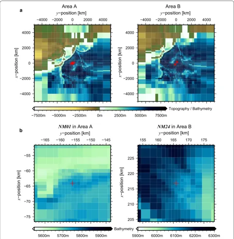
Fig. 1 Bathymetry maps and site locations. a Regional bathymetry map based on ETOPO1 (Amante and Eakins 2009) with contour lines for seafloor
Table 1 Information on the OBEM and EFOS sites and data used in this study
Site ID Instrument Institute Observation
phase Latitude Longitude Depth (m) Sampling interval (s) Available period/remarks
NM01 OBEM ERI Pilot 39°12.01′N 154°47.09′E 5756 60 20/06/2010–07/03/2012 ERI 2nd 39°11.93′N 154°45.88′E 5751 60 05/09/2012–22/08/2013 ERI 3rd 39°11.79′N 154°45.67′E 5751 10, 60a 31/08/2013–06/09/2014
Average 39°11.91′N 154°46.21′E 5754
EFOS ERI 2nd 39°12.02′N 154°45.91′E 5748 1 10/09/2012–13/09/2014b
E-dipole: 1.8 km, N113°E
NM02 OBEM ERI Pilot 39°42.09′N 153°21.17′E 5734 60 25/06/2010–26/02/2012
JAMSTEC 2nd 39°42.68′N 153°21.21′E 5730 60 Unavailablec
NM03 OBEM ERI Pilot 38°45.84′N 155°54.73′E 5765 60 Unavailabled
ERI 2nd 38°45.03′N 155°54.06′E 5757 10, 60a Unavailabled
ERI 4th 38°45.58′N 155°55.15′E 5763 10, 60a 24/09/2014–13/09/2015
EFOS ERI Pilot 38°45.81′N 155°54.69′E 5766 1 Unavailablee
2nd 38°45.81′N 155°54.69′E 5766 1 Unavailablee
E-dipole: 3.3 km, N111°E
NM04 OBEM ERI Pilot 38°12.67′N 154°11.40′E 5946 60 20/06/2010–26/11/2011
ERI 1st 38°12.78′N 154°12.21′E 5956 10, 60a Unavailabled
NM05 OBEM ERI Pilot 40°15.00′N 155°24.40′E 5615 60 25/06/2010–26/02/2012 ERI 2nd 40°15.22′N 155°24.78′E 5619 10, 60a 21/08/2012–24/08/2013
Average 40°15.11′N 155°24.59′E 5621
NM06 OBEM ERI 3rd 39°29.62′N 155°42.82′E 5599 10, 60a Unavailabled
NM07 OBEM ERI 3rd 41°07.73′N 156°01.15′E 5632 10, 60a 31/08/2013–04/06/2014
NM08 OBEM ERI 3rd 40°32.67′N 156°19.35′E 5546 10, 60a 31/08/2013–03/06/2014
NM09 OBEM ERI 3rd 39°47.35′N 156°34.84′E 5547 10, 60a 31/08/2013–02/06/2014
NM10 OBEM ERI 3rd 39°03.19′N 156°58.83′E 5734 10, 60a 31/08/2013–02/06/2014
NM11 OBEM ERI 3rd 38°15.05′N 157°17.31′E 5704 10, 60a 31/08/2013–02/06/2014
NM12 OBEM JAMSTEC 2nd 40°49.04′N 157°06.58′E 5511 60 30/08/2012–26/08/2013
NM13 OBEM ERI 3rd 40°01.51′N 157°28.38′E 5535 10, 60a 31/08/2013–06/06/2014
NM14 OBEM JAMSTEC 2nd 39°02.44′N 158°00.76′E 5512 10, 60a Unavailablee
ERI 3rd 39°02.48′N 158°00.12′E 5510 10, 60a 31/08/2013–15/09/2014
EFOS ERI 2nd 39°02.64′N 158°00.61′E 5509 1 06/09/2012–18/09/2014b
E-dipole: 2.0 km, N107°E NM15 OBEM JAMSTEC 2nd 40°21.17′N 158°24.51′E 5578 60 28/08/2012–27/08/2013
NM16 OBEM ERI 2nd 41°01.33′N 159°11.19′E 5577 10, 60a 27/08/2012–27/07/2014
EFOS ERI 2nd 41°01.27′N 159°11.20′E 5578 1 04/09/2012–17/09/2014
E-dipole: 1.9 km, N103°E NM17 OBEM JAMSTEC 3rd 39°46.15′N 159°51.75′E 5541 60 01/09/2013–06/06/2014
NM18 OBEM ERI 1st 30°10.96′N 161°17.44′E 5983 60 01/12/2011–18/01/2013
NM19 OBEM ERI 1st 29°09.09′N 161°46.51′E 5930 60 01/12/2011–02/09/2013
NM20 OBEM JAMSTEC 1st 30°38.50′N 162°32.72′E 5970 60 01/12/2011–01/09/2013 ERI 3rd 30°38.58′N 162°33.67′E 5968 60 Unavailablee
NM21 OBEM ERI 1st 29°32.51′N 162°51.55′E 5986 60 Unavailabled
NM22 OBEM JAMSTEC 1st 32°56.94′N 163°48.85′E 6188 60 01/12/2011–30/08/2013 NM23 OBEM JAMSTEC 1st 31°55.52′N 164°24.57′E 6073 60 01/12/2011–31/08/2013 NM24 OBEM ERI 1st 33°13.24′N 165°15.65′E 6118 60 01/12/2011–27/08/2013b
NOMan project cruises. The bathymetry map based on the MBES data is also shown in Fig. 1b.
Two kinds of EM instruments were utilized in this experiment: ocean bottom electromagnetometers (OBEMs) and electric field observation systems (EFOSs). OBEMs measure the time variations of three compo-nents of the magnetic field, two horizontal compocompo-nents of the electric field, two components of instrumental tilt, and temperature. These instruments were deployed to the seafloor via free fall from the sea surface and were retrieved when they rose to the surface due to buoy-ancy after releasing an anchor. Most of the OBEMs recorded data with a sampling interval of 60 s. For some OBEMs, the sampling interval was first set at 10 s and then switched to 60 s, controlled by a timer. This func-tion helps to optimize battery power consumpfunc-tion more efficiently because the magnetometer is powered on intermittently for only a few seconds around the time of sampling. The 10-s sampling recordings provide shorter-period data that are sensitive to shallower parts of the oceanic lithosphere. There were also sites where the OBEMs were deployed iteratively to collect longer time series data (Table 1). The positions between these sites on the seafloor were slightly different from each other (0.4– 2.0 km) because they were settled via free fall. We there-fore regarded the averages as the representative positions of the sites. As addressed later, these differences in posi-tion are not critical in the analysis for study of mantle structure and topographic effects.
EFOSs measure just one component of the electric field, but with a much longer dipole (2–3 km for the NOMan experiment) than that of the OBEMs (~5.4 m), and therefore yield better signal-to-noise (S/N) ratios (Utada et al. 2013). An EFOS consists of a recorder and a cable drum attached to an anchor. The EFOS is deployed to the seafloor via free fall, and the cable drum is then caught and towed by a remotely operated underwater vehicle (ROV) KAIKO 7000II to extend the cable that generates the long electric dipole. An EFOS was deployed at NM03 in 2010 as the part of the pilot survey. In 2012,
the recorder was replaced and the measurements were continued. Three additional EFOSs were deployed, at NM01, NM14, and NM16. The direction of the cable extension was restricted by the recorder side because of the instrumental design and a technical reason of the ROV operation (Utada et al. 2013). All of the EFOS recorders happened to settle facing between N40°E and N170°E after free fall deployment; therefore, the cables were extended approximately in the N110°E direction (Table 1), which is subparallel to the direction of Pacific Plate motion. The EFOS recorders at sites NM01, NM14, and NM16 were retrieved using the ROV KAIKO 7000II in 2014, and the recorder at NM03 was retrieved using ROV KAIKO Mk-IV in 2015. Further information about the EFOSs is listed in Table 1.
The recovered time series data were first processed for quality control. Abnormal fluctuations, such as spikes and rectangular steps in raw time series data, were detected by eye through comparing different field com-ponents, and spikes were then linearly interpolated and steps were shifted to reduce discontinuity. The instru-mental clock was compared with coordinated univer-sal time (UTC) via global positioning system (GPS) just before deployment and after retrieval. The detected clock shift was corrected, based on the assumption that the shift accumulated linearly over time. For the OBEMs, the coordinate system was adjusted to a geographical one; the instrumental tilt was corrected using tilt angle data through Euler rotation, and the horizontal coordinate system was then rotated using the magnetic field declina-tion predicted from the internadeclina-tional geomagnetic refer-ence field (IGRF) (IAGA Working Group V-MOD 2010). Coordinate system conversion was not applied to the EFOS data because the EFOSs measured only one com-ponent of the electric field.
Magnetotelluric analysis
The MT response Z(r, T) is defined as a 2 × 2 complex-valued tensor transfer function between the horizontal electric E(r, T) and magnetic B(r, T) fields,
For EFOS data, the position is that of the recorder, and the dipole length and direction from the recorder are noted in remarks. The positions given in italicized characters are the representative positions for each site. Water depths at each site were retrieved from the up-to-date compilation of available MBES data, and the values for some sites are therefore slightly different from those previously reported by Baba et al. (2010, 2013a)
a Sampling intervals were changed during observation (see text for details)
b Includes unavailable sections
c Failed to retrieve data
d Failed to retrieve the instrument
e Noisy
Table 1 continued
Site ID Instrument Institute Observation
phase Latitude Longitude Depth (m) Sampling interval (s) Available period/remarks
where r is the observed position and T is the period. The responses were estimated for each OBEM site using a bounded influence algorithm (Chave and Thomson 2004). The magnetic field data from the Kakioka obser-vatory (KAK) were employed as a remote reference to reduce the effects of site-dependent noise in the local (OBEM) magnetic field data. We also applied a general-ized remote reference method based on two-stage pro-cessing (Chave and Thomson 2004). In the first stage, a transfer function between the local and remote hori-zontal magnetic fields was estimated, and in the second stage, the MT responses were estimated as a transfer function between the local observed electric field and the local horizontal magnetic field estimates predicted from the inter-site magnetic transfer function obtained in the first stage. The generalized remote reference method sig-nificantly improved the quality of the MT response esti-mation for periods shorter than ~500 s at the sites where 10-s sampling data were available. The final responses for each period were taken from those obtained using either the normal or generalized remote reference method with higher coherence. Finally, the MT responses were obtained for the period range between 53.3 and 163,840 s
(1)
E(r,T)=Z(r,T)B(r,T), (the available range depends on the site). The longest
available period is limited to 163,840 s, although data for more than 3 years were used, mainly because the S/N ratio of the electric field measured by the OBEMs becomes quite low with fluctuations over longer periods.
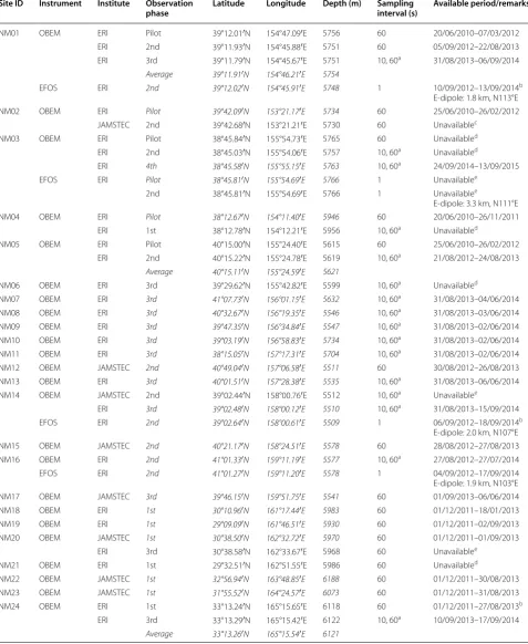
We examined the influence of the different positions of the OBEMs deployed in the different observation phases by comparing the MT responses estimated from data for each observation phase and from all observation phases. For NM01, data are available from three observation phases (Table 1). The distances between pairs of OBEM positions are 0.4–2.0 km (Fig. 2a). The resulting MT responses all agree within the 95% confidence interval (Fig. 2b). These results suggest that, in the present study, relocation error is not critical in this analysis of mantle structure and topographic effects. Therefore, we used the MT responses estimated from all available observa-tion phase data to represent the response at each site and used the average position for the MT response simula-tion in the following analysis.
The OBEM magnetic field data and EFOS data at the same sites were also processed jointly to yield a scalar MT response between the electric field along the EFOS dipole and the OBEM magnetic field component perpendicular to the EFOS dipole. In addition, the geomagnetic depth
a b
Fig. 2 a OBEM locations and the average for NM01 plotted on a bathymetry map. b Comparison of the MT responses at NM01 obtained from all
sounding (GDS) response, which is the transfer func-tion between the vertical component and the horizontal component of the magnetic field, was estimated for each OBEM site and for the seafloor observatory at the North Western Pacific (NWP) (Toh et al. 2006). These responses were estimated for periods longer than ~105 s and are
therefore useful to evaluate deeper structure. Matsuno et al. (2017) have provided a detailed analysis of the data and discussion of the structure of the mantle transition zone. Therefore, in this study, we focus on analysis of the MT responses obtained with the OBEM data and discus-sion of the upper mantle structure.
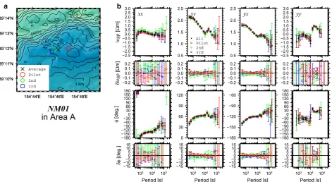
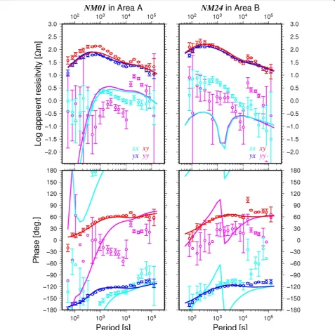
Examples of the MT responses representative of each area (NM01 for Area A and NM24 for Area B) are plot-ted in the form of apparent resistivity and impedance phase sounding curves to reveal the variation as a func-tion of period (Fig. 3). See Additional file 1: Figure S1 for the sounding curves of all sites. In Fig. 4, polar dia-grams of the apparent resistivity (Swift 1967) are plot-ted, as well as phase tensor ellipses (Caldwell et al. 2004), on a bathymetric map for two selected periods (640 and 5120 s) to illustrate the lateral variations of the tensor MT responses.
We first show the overall features of the sounding curves. With periods shorter than about 500 s (Fig. 3), the apparent resistivity and phase in the major elements decrease with decreasing period, which suggests that the uppermost layer is relatively conductive, likely associated with the crust including a thick (~400 m) pelagic sedi-ment layer (Shinohara et al. 2008). The apparent resistivi-ties show a peak at around 500 s and then decrease with increasing period (Fig. 3). This feature is typical for oce-anic mantle that consists of cool, resistive lithosphere and underlying hotter, more conductive asthenosphere (e.g., Filloux 1977). The peak of the apparent resistivity is higher for Area B than for Area A (Fig. 3). The responses look similar between sites within each area, but the spatial variation tends differ somewhat between Area A and Area B. For example, the phase tensors at 5120 s tend to elon-gate in the northeast–southwest direction in Area A, but form a more circular shape in Area B (Fig. 4). These obser-vations suggest a difference in the upper mantle structure at a scale beyond the array size. Splitting between the off-diagonal elements suggests the effect/s of lateral hetero-geneity and/or anisotropic structure. This phenomenon is smaller for Area B, which is more distant from the coast-lines; therefore, the coast effect is likely a possible cause. In fact, our previous study showed that splitting in the responses for Area A is partly explained by the topogra-phy, including coastlines (Baba et al. 2013a). However, for Area A, the splitting tends to be slightly more significant at the western sites, NM01, NM02, and NM04 (Fig. 3; Addi-tional file 1: Figure S1), and this feature is not reproduced
well with the topographic effect alone (Baba et al. 2013a), which suggests the presence of lateral heterogeneity within the array or at a slightly larger scale. At periods of about 104 s, both the apparent resistivities and phases, especially
for the xy and yy elements, abruptly change (Fig. 3). This feature is more significant for Area B, which is the most distant from the reference site (KAK). It is likely caused by imperfect reduction of Sq effects (Shimizu et al. 2011). Therefore, we have down-weighted the responses within the period range of 104–105 s, where the Sq effects
domi-nate, in later analysis. Nevertheless, the splitting between the off-diagonal elements likely decreases with increasing periods, which suggests that the deeper part of the upper mantle tends to be more uniform laterally.
Topographic effect correction and inversion
We estimated one-dimensional (1-D) isotropic electrical conductivity profiles of the mantle for Area A and Area B separately, which fit the MT response averaged in each array, by applying an iterative topographic effect correc-tion. The 1-D profile estimated by this procedure should be a representative of average 1-D structure of possi-bly laterally heterogeneous (and/or anisotropic) man-tle beneath each array. We do not argue that the manman-tle structure is one-dimensional as we discuss possible lat-eral heterogeneity and anisotropy later. This procedure is critical to obtain a reliable subsurface structure model because the large contrast in conductivity between sea-water and crustal rocks can severely distort the EM field at the seafloor. This procedure is based on our previous studies (Baba and Chave 2005; Baba et al. 2010, 2013a, c) and consists of four steps. The procedure of these steps is iterated until the results converge to obtain the final 1-D profile, as described below.
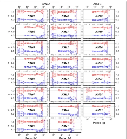
In Step 1, we first calculate a scalar MT response from the tensor MT response at each site. We adopt the square root of the determinant of the tensor MT response,
Zdet=ZxxZyy−ZxyZyx, which is an invariant to rota-tion of the horizontal coordinate system, following the methods of our previous studies (Baba et al. 2010, 2013a). Rung-Arunwan et al. (2016) demonstrated that another rotational invariant based on the sum of squared ele-ments, Zssq=
robust to galvanic distortion. However, the distortion indicators, γ =Zssq2 /Z2det (Rung-Arunwan et al. 2016), are
real and nearly equal to unity independently of period for all sites, which indicates that Zdet is almost identical to
Zssq (Fig. 5) and that the present dataset is affected little
is generally much more homogeneous geologically than continental crust that has undergone tectonic processes and erosions. The estimates of Zdet(r,T) for all sites are
then averaged in each array for each period.
In Step 2, Occam’s inversion (Constable et al. 1987) is applied to the averaged response Z¯
det(T) to obtain a rep-resentative 1-D profile. The error floor of 2.5% of
Z¯det
is
applied, except for the periods between 104 and 105 s, to
which an error floor five times larger (12.5%) is applied, because the responses in these periods are likely dis-torted by imperfect reduction of Sq effects, as described above. The conductivity at ~30 km depth is constrained to be 10−3.5 S m−1 in the inversion, following our
previ-ous studies (Baba et al. 2010, 2013a), because the inver-sion of Z¯
no doubt that the cold lithosphere exhibits very low con-ductivity (e.g., Baba et al. 2010, 2013a; Cox et al. 1986). The inversion did not converge if the target misfit was set to 1.0. Then, the target misfit was set to 1.24 and 1.25 for Area A and Area B, respectively, which correspond to the 99% confidence limit of χ2 misfit. The uncertainty
of the conductivity of each layer is estimated by evalu-ating the distribution of the acceptable models obtained through numerous inversion runs with different con-straints, following our previous studies (Baba et al. 2010, 2013a).
In Step 3, the topographic effect is simulated. A two-stage three-dimensional (3-D) forward modeling approach (Baba et al. 2013c) is applied to incorporate the effects of regional large-scale topography and local small-scale topography. The lateral dimensions of the regional model are 10,000 km × 10,000 km, and the horizontal mesh in the central area that includes the array is 50 km × 50 km. The local model is as large as 350 km × 350 km, with topography in the vicinity of each site based on MBES data and is also incorporated with a finer mesh (1 km × 1 km in the central area) in the sec-ond stage forward modeling (Baba et al. 2013c). Figure 6a
shows the regional topography models for the two areas, and Fig. 6b shows examples of the local topography model at a particular site for each array. The regional model includes the East Asian coastlines and major topographic features such as abyssal rises and trenches. The local models incorporate finer-scale topographic changes, such as linear hills and valleys subparallel to the past seafloor spreading ridge. The conductivity values of seawater and land crust are set to 3.2 and 0.01 S m−1,
respectively. The 1-D profile obtained in Step 2 is incor-porated in the subsurface structure.
In Step 4, the topographic distortion terms for each site, D(r,T), are calculated from the 3-D and 1-D forward responses Zpre
3−D(r,T) and Z pre
1−D(T), assuming that the 3-D response to be observed is expressed by multiplication of the surface 3-D topographic distortion and the response to the subsurface 1-D structure,
Then, the observed responses Zobs(r,T) are corrected as, (2) D=Zpre
3−D
Zpre 1−D
−1
.
(3) Zcor=D−1Zobs.
0.0 0.1 0.2 0.3 0.4 0.5
Swift’s impedance skew
0 2 4 6 8 10
Phase tensor skew angle [deg.]
T=5120 [s]
1, 100 [Ωm]
T=640 [s]
30, 60 [deg.]
Area A
logρ polar diagram Phase tensor ellipses
1, 100 [Ωm] 30, 60 [deg.]
Area B
logρ polar diagram Phase tensor ellipses
We evaluate the root mean squared (RMS) misfit between the observed (non-corrected) and predicted responses in terms of log apparent resistivity log ρ and impedance
phase φ, (4)
where Nd is the total number of data points for Z involving
four elements of the tensor, the number of available peri-ods, which depends on the site, and the number of sites. The parameters δlogρ and δφ are the standard errors,
to which the error floor is applied. Error floors are set to 2.5% for the off-diagonal elements of Z, for the diagonal elements, are set to the absolute value of 0.01 for periods
shorter than 3000 s, and 5.0% for the longer periods. These criteria are based on our experience regarding the approxi-mate accuracy of regional 3-D forward modeling. How-ever, for periods between 104 and 105 s, the error floors are
increased by a factor of five, i.e., to 12.5 and 25.0% for off-diagonal and off-diagonal elements, respectively, for the same reason as for the 1-D inversion in Step 2.
−75 −70 −65 −60 −55
x
−position [km]
−165 −160 −155 −150 −145
y−position [km] NM01 in Area A
5600m 5700m 5800m 5900m
Bathymetry b
205 210 215 220 225
x
−position [km
]
155 160 165 170 175
y−position [km] NM24 in Area B
5900m 6000m 6100m 6200m 6300m −4000
−2000 0 2000 4000
x
−position [km]
−4000 −2000 0 2000 4000
y−position [km]Area A
a
−4000 −2000 0 2000 4000
x
−position [km]
−4000 −2000 0 2000 4000
y−position [km]Area B
−7500m −5000m −2500m 0m 2500m 5000m 7500m
Topography / Bathymetry
Fig. 6 a Regional topography models for Area A and Area B. b Example local topography models for NM01 in Area A and NM24 in Area B (only the
Results
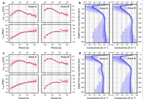
Figure 7a presents Zdet(r,T) and Z¯det(T) from Area A and Area B, as obtained in Step 1. The averaged responses differ significantly between the two areas, and this dif-ference is beyond the dispersion between sites within each area. These features remain after topographic effect correction (Fig. 7c), which suggests that the subsurface structures differ significantly between the areas. The top-ographic effect correction increased the apparent resis-tivity at longer periods for both areas, but the change is larger for Area A than for Area B. Therefore, this change should mainly be attributed to relatively large-scale topo-graphic effects, such as the coastlines west of the study areas. The dispersions in the responses within each array, which are larger with shorter periods, changed lit-tle with topographic effect correction. This result indi-cates that local topographic effects, which should affect the responses in shorter periods more strongly, are not as significant as the regional topographic effects and
that the dispersions are caused by lateral heterogeneity in subsurface (but relatively shallow) structure. Because the dispersion is very small within Area B, the subsurface structure beneath Area B is inferred to be more uniform laterally.
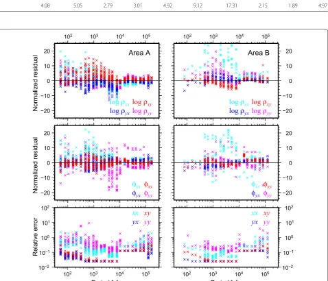
The topographic effect correction and inversion proce-dure was iterated twice. Changes in RMS misfit against the iterations are listed in Table 2. Figure 8 shows the residuals between the responses observed and predicted from the final model, which were normalized based on the relative errors δZ/|Z| after applying the error floors. The errors for each element are of a similar level for the two areas, such that the difference in the RMS mis-fit approximately reflects the difference in the absolute model fit. The RMS misfit decreased significantly at the first iteration and then slightly increased again at the second iteration; therefore, we took the result at the first iteration as the final model. The reduction of the misfit from the initial to the final model is as small as 14% for
−30
Depth from sea surface [km]
10−5 10−4 10−3 10−2 10−1 100 Conductivity [S m−1] 10−5 10−4 10−3 10−2 10−1 100
Depth from sea surface [km]
10−5 10−4 10−3 10−2 10−1 100 Conductivity [S m−1] 10−5 10−4 10−3 10−2 10−1 100
Conductivity [S m−1] 10−5 10−4 10−3 10−2 10−1 100
Conductivity [S m−1] 10−5 10−4 10−3 10−2 10−1 100
Area B
Area A and 2% for Area B. This small reduction indicates that the initial 1-D models were good enough compared to other choices for the initial model, such as a uniform half space, which is frequently used for inversion analyses (Baba et al. 2013a). For Area B, the RMS misfit is almost twice of that for Area A, and the reduction was smaller. This difference occurs because for Area B, the RMS misfit
of the xx element is extremely high compared to that for the off-diagonal elements (Table 2; Fig. 8). The partial RMS misfits for the off-diagonal elements for Area B were smaller than those for Area A, and the reductions were as large as 9–38%.
The predicted responses explain the overall features of the observed responses, although there are some Table 2 The RMS misfit against the iteration
Iteration Area A Area B
Total xx xy yx yy Total xx xy yx yy
0 4.66 5.40 4.86 3.02 4.98 9.32 17.51 2.35 3.03 5.16
1 3.99 4.80 3.19 2.54 4.92 9.10 17.28 2.15 1.88 4.94
2 4.08 5.05 2.79 3.01 4.92 9.12 17.31 2.15 1.89 4.97
10−2
10−1
100
101
102
Relative error
102 103 104 105 Period [s]
xx
xy
yx
yy
−20−10 0 10 20
Normalized residual
φ
φ
xxyxφ
φ
xyyy −20−10 0 10 20
Normalized residual
102 103 104 105
Area A
log
ρ
xxlog
ρ
xylog
ρ
yxlog
ρ
yy10−2 10−1 100 101 102
102 103 104 105
Period [s]
xx
xy
yx
yy
−20 −10 0 10 20φ
xxφ
xyφ
yxφ
yy−20 −10 0 10 20 102 103 104 105
Area B
log
ρ
xxlog
ρ
xylog
ρ
yxlog
ρ
yyFig. 8 Normalized residuals in four elements of the MT responses for Area A (left) and Area B (right). Colors indicate the different elements, as specified in the legend. Top and middle panels are those for the log apparent resistivity, (log ρobs− log ρpre)/δ log ρ, and phase, (φobs−φpre)/δφ,
significant differences between them (Figs. 3, 8). Rela-tively large misfits are mainly seen with periods shorter than several thousand seconds. For Area A, the splitting between the xy and yx (off-diagonal) elements or the xx and yy (diagonal) elements of calculated responses is smaller than the observed splitting (Fig. 3; Additional file 1: Figure S1), as was pointed out in our previous study based on the pilot survey data (Baba et al. 2013a). For Area B, in contrast, the off-diagonal elements are very well reconstructed by the model. However, as shown in Fig. 3, the predicted apparent resistivities for the two diagonal elements are similar and much smaller than the observed values. They are largely depressed and accom-panied by a large phase change at ~2000 s. In addition, the observed apparent resistivity for the xx element is higher, and its errors are smaller than those for the yy element. These values resulted in the high partial RMS misfit for the xx element (Fig. 8; Table 2). These features cannot be reproduced by the topographic effect alone and therefore must be attributed to lateral heterogeneity and/or anisotropy of the subsurface structure. We expect future studies to better explain these features.
The 1-D profiles before and after the topographic effect correction for each area are shown in Fig. 7b, d. As anticipated from the observed sounding curves, the profiles were characterized by three layers, consisting of the uppermost conductive layer, the resistive lithospheric mantle, and the conductive asthenospheric mantle. As a result of topographic effect correction, the conduc-tivity of the asthenospheric mantle decreased from the initial profile to the final profile. This reduction is more
significant for Area A. Major differences in the final pro-files between the two areas are: (1) the thickness of the resistive layer and (2) the conductivity values at the peak in the upper mantle. The definition of the thickness of the resistive layer is somewhat ambiguous because the profiles change smoothly with depth, and the gradient is controlled by the smoothness constraint in the inver-sion as well as by the data. If we define this thickness as the depth where the conductivity become greater than 0.01 S m−1, that thickness is ~90 km for Area A and
~100 km for Area B. It is quantitatively certain that the resistive layer in Area A is thinner than that in Area B. In the highly conductive zone below the resistive layer, the depth-dependent trend is much more gradual, with val-ues of 0.02–0.03 S m−1 at depths of 100–150 km in Area
A, and ~0.05 S m−1 at depths of 150–200 km in Area B.
Discussion
Update of the model for Area A
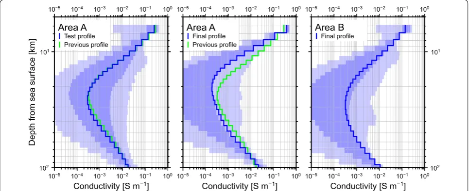
The number of available sites for Area A was increased from four in the previous study (Baba et al. 2013a) to 16 in this study with completion of the main observa-tion phase. The variaobserva-tion of observed MT responses in the array is of a similar level with that of the pilot sur-vey array (four western sites). The obtained 1-D profile for mantle depth is also similar to the previous profile, which indicates that extension of the data to include shorter periods in this study did not affect the evaluation of the mantle, as is our main target. However, significant improvement is apparent in the uncertainty for the shal-lowest part of the profile (Fig. 9), which indicates that the
101
102
Depth from sea surface [km]
10−5 10−4 10−3 10−2 10−1 100
Conductivity [S m−1]
10−5 10−4 10−3 10−2 10−1 100
Area A
10−5 10−4 10−3 10−2 10−1 100
Conductivity [S m−1]
10−5 10−4 10−3 10−2 10−1 100
Area A
101
102 10−5 10−4 10−3 10−2 10−1 100
Conductivity [S m−1] 10−5 10−4 10−3 10−2 10−1 100
Area B Test profile
Previous profile
Final profile Previous profile
Final profile
conductive oceanic crust is better constrained by the new data and thus that the conductivity values are more reli-able. We ran an inversion for a test with the present data but excluded some data points at periods shorter than 160 s, as in the previous study. The resulting profile is very similar to the previous one, but the uncertainty of the final profile in this study is much smaller.
This improvement enables us to probe the uppermost mantle and crust (down to ~10 km below the seafloor) more reliably, even at the deep seafloor. The uppermost layer for Area A seems to be more conductive than those for Area B, although the uncertainty for Area B is larger than that for Area A (Fig. 9). Shinohara et al. (2008) con-ducted a seismic survey in the eastern end of our array in Area A and showed that the sediment layer is as thick as ~400 m. The seismic survey by Ohira et al. (2017) along a line 150 km southeast of our array in Area B showed that the thickness of the sediment layer is ~300 m. Both stud-ies reported similar characters; the P-wave velocity struc-ture in the crust below the sediment indicated typical oceanic crust, except for the transitional layer from the crust to the mantle. Although our models do not resolve the shallowest layer, which is thinner than 1 km, the thin but very conductive sediment layer can influence the mean conductivity in the uppermost layer in the inver-sion. Therefore, the difference between the shallower parts of the profiles from the two areas may be ascribed to the difference in the thickness of the sediment layer.
Possibilities of lateral heterogeneity and anisotropy within each area
The MT responses show some degree of spatial varia-tions within each array (Figs. 4, 7a, c), which suggests the presence of lateral heterogeneity and/or anisotropy in conductivity. Although detailed 3-D and anisotropy analyses are now underway in subsequent studies, here we argue some implications regarding the lateral hetero-geneity and anisotropy in the upper mantle for each area. Figure 10 shows the spatial distribution of the residuals between the apparent resistivity of Zdet(r,T) after the topographic effect correction and the forward response to the final 1-D profiles for each area. At three selected periods, 1280, 2560, and 5120 s, the apparent resistivity decreases with increasing period for both Area A and Area B, which suggests that the data for these periods may be responsible for the depths from the base of resis-tive layer to the underlying conducresis-tive zone. The radii of the colored circles in the figure are normalized for the standard error of the log apparent resistivity to dem-onstrate that the residuals with larger circles are more reliable than those with smaller circles. For Area A, the spatial trend is not very clear at 1280 s, but the eastern sites are more conductive at longer periods. For Area
B, the northeastern region tends to be more conductive with all three periods, although the spatial variation is smaller than that in Area A. The overall difference in the data between Area A and Area B is significantly larger than the dispersion of the data within each array (Figs. 7, 10). Therefore, the major difference in the 1-D profiles between the two areas is a robust feature.
Anisotropy in the lithosphere and asthenosphere is an important property to assess mantle dynamics, although observational evidence is available only from relatively young oceanic mantle in the eastern Pacific region (Evans et al. 2005; Baba et al. 2006a, b; Naif et al. 2013). Recent experimental studies have also demonstrated that hydrous olivine and partially molten rock can be highly anisotropic under the temperature and pressure condi-tions of the asthenosphere (e.g., Dai and Karato 2014; Zhang et al. 2014; Pommier et al. 2015). Therefore, the possibility of anisotropy should not be ruled out for the old oceanic mantle in our study areas. Qualitatively, we can infer that the anisotropy in the study areas, if it
−0.20 −0.15 −0.10 −0.05 0.00 0.05 0.10 0.15 0.20
log (ρdet / ρ1−D)
T=5120 [s] T=2560 [s]
T=1280 [s] Area A Area B
Fig. 10 Residuals between the log apparent resistivity of Zdet after
exists, may be weaker than that observed in the south-ern East Pacific Rise (Evans et al. 2005; Baba et al. 2006a, b) because the major (off-diagonal) elements of the observed MT responses show only slight variation with rotation in horizontal coordinates (Fig. 4). Therefore, special care is necessary in examining the existence and degree of anisotropy more quantitatively, because the present MT data are affected by the 3-D topography, and mutual coupling between the topographic effect and the anisotropic mantle structure must be considered. Such a careful study is currently in progress to explore how the topography and possible anisotropy affect MT responses. Details of this analysis and its results will be reported elsewhere.
Spatial dependence of electrical conductivity of the upper mantle in the northwestern Pacific and its implication for the lithosphere–asthenosphere system
The electrical conductivity of the upper mantle differs between Area A and Area B, as demonstrated in the pre-vious section. The major differences in the upper mantle are the thickness of the resistive layer and the high con-ductivity beneath the resistive layers. We confirmed that these differences are significant and not artifacts because of the high conductivity at the uppermost layers, through synthetic inversion tests (see Additional file 2: Figure S2). The seismological observations of the NOMan project have also revealed noticeable differences in shear-wave velocity structure between the two areas through surface wave tomography. The upper high-velocity layer tends to be thicker for Area B than for Area A, and the underly-ing low-velocity zone tends to show slower velocities for Area A than for Area B (Isse et al. 2017). The electrical conductivity and seismic slowness in the upper mantle can both be enhanced primarily by temperature increase. Therefore, the trends in the thickness of the upper resis-tive layer and the high-velocity layer between the two areas are qualitatively consistent, as the cool lithospheric mantle is thinner for Area A than for Area B. However, the conductivity and the velocity in the underlying con-ductive and low-velocity zone beneath the two areas appear to be opposite what would be explained by the thermal effect alone. This apparent inconsistency strongly suggests that other factors, such as volatile content and/ or degrees of partial melting, differ in the mantle beneath the two areas. This observation also highlights the impor-tance of further joint interpretation of seismic and EM results.
We next evaluate the spatial dependence of electri-cal conductivity across a wider region by comparing the 1-D electrical conductivity profiles for four areas of the northwestern Pacific. Two additional areas, Area C and Area D, are in the Pacific basin off the Bonin Trench
(the representative crustal age is ~147 Ma) and off the Japan Trench (~135 Ma), respectively (locations shown in Fig. 1), where seafloor MT data were collected in past experiments (Baba et al. 2010, 2013b). The representa-tive 1-D profiles for Area C and Area D were previously obtained following a similar procedure to that used in the present study, but they were re-estimated in this study using the same up-to-date procedure as that applied for Area A and Area B to avoid potential artifacts due to slight differences in procedure. However, differences from the previous profiles are negligible.
Figure 11 shows the 1-D profiles for the four areas, which further highlight the variation in resistive layer thickness (the profiles in machine-readable format are given in Additional file 3: Table and the sounding curves for Z¯det(T) (red) and Zdet(r,T) for all sites in the four areas are shown in Additional file 4: Figure S3). Area C shows the thickest resistive layer, which was also con-firmed to be a robust feature by 3-D inversion analysis (Tada et al. 2014), and that of Area D falls between those of Area B and Area C. All four models differ significantly from each other. The conductivity values of the under-lying high conductive zones for Area C and Area D are around 0.04–0.05 S m−1, which is close to that of Area
A. That of Area B is slightly more conductive than the others.
The differences in resistive layer thickness between these four areas cannot be explained by the tempera-ture differences of the corresponding lithospheric ages under a framework of the cooling of homogeneous man-tle through thermal conduction. We have already argued this point based on the comparison of the earlier pro-files for Area A and Area C (Baba et al. 2013a), and this comparison of four areas further strengthens this inter-pretation. Baba et al. (2013a) argued that if the mantle beneath Area A is “normal,” as expected from the plate cooling model, the lithosphere beneath Area C is abnor-mally thick. However, adding Area B and Area D to this comparison demonstrates that the resistive layer beneath Area A is the thinnest, and therefore represents the opposite end-member rather than the average among the four areas explored thus far. It is now more doubtful that Area A represents “normal” mantle in the old northwest-ern Pacific.
To demonstrate these inferences more clearly, we simu-lated the 1-D electrical conductivity profiles for several thermal structure models with the representative lith-ospheric age for each area and plotted these profiles in Fig. 11 (dashed lines). We applied simple 1-D cooling of a homogeneous, thermally conductive plate, assuming a potential temperature of 1350 °C and thermal diffusiv-ity of 30 km2 Myr−1 (Turcotte and Schubert 2002). The
adiabatic temperature gradient of 0.3 °C km−1 was
super-imposed onto this thermal profile. The mantle electri-cal conductivity was assumed to be represented by that of olivine. We applied the electrical conductivity model for olivine by Gardés et al. (2014), which was obtained by compiling published experimental results. The water content dissolved in olivine was assumed to be 0.01 wt.%, which is thought to be a typical value for mid-ocean ridge basalt (MORB) source mantle (Hirschmann 2010). Note that there are two competing groups that show signifi-cantly different results for the conductivity measurement
of hydrous olivine, and therefore, selection of the labora-tory model leads different impacts of water on the con-ductivity simulation. Olivine concon-ductivity calculated using the model of Gardés et al. (2014) falls in a middle ground between values those calculated using the models of the two competing groups (Wang et al. 2006; Yoshino et al. 2009) in a case for water content of 0.01 wt.% at 1200 °C (see their Fig. 1). In the simulation, we consid-ered only the solid-state mantle and the effects of tem-perature and water on that mantle. However, we do not rule out the possible contribution of partial melting due 0
50
100
150
200
250
300
Depth from sea surface [km]
10−5 10−4 10−3 10−2 10−1 100
Conductivity [S m−1]
Area C
(147 Myr)
0
50
100
150
200
250
300 10−5 10−4 10−3 10−2 10−1 100
Conductivity [S m−1]
Area D
(135 Myr) 0
50
100
150
200
250
300
Depth from sea surface [km]
10−5 10−4 10−3 10−2 10−1 100
Area A
(130 Myr)h=80 [km] h=100 [km] h=125 [km] h=150 [km] h=200 [km] h=300 [km]
0
50
100
150
200
250
300 10−5 10−4 10−3 10−2 10−1 100
Area B
(140 Myr)
to the presence of water and carbon dioxide (e.g., Sifré et al. 2014).
The calculated electrical conductivity profiles for any h are almost identical between the four different repre-sentative ages, because the thermal structure is almost identical in the range of ages compared here. However, the results for different values of h showed significantly different conductivity profiles. The inversion profile for Area A falls between the simulated profiles for h of 80 and 100 km. For Area B, the inversion profile is in between the profiles for h of 100 and 125 km. For Area D, it mostly corresponds to the simulated profiles for h of 200 and 300 km, which are almost the same. The resistive layer for Area C is much thicker than the simulated profile for h of 300 km, which suggests that it is more consist-ent with a cooling half space rather than a cooling plate, as discussed in previous studies (Baba et al. 2010, 2013a). This result suggests that the transition from the resistive to high-conductivity zones is mainly controlled by h. It is impossible to represent the 1-D profiles for all areas by a thermal model with a single value of h. In other words, it is likely that the thickness of the cool thermal lithosphere differs between these areas. If the appropriate values of h are chosen, the simulated profiles with the same value of potential temperature fit the high-conductivity zone well for all areas, although the inversion profile for Area B is slightly higher than the simulated profile at depths between 150 and 200 km. This observation suggests that the asthenospheric mantle in this region is rather homo-geneous in potential temperature and chemical composi-tion, except for Area B.
Bathymetry subsidence and heat flow data seem to be consistent partly but not perfectly with the significant trend in the resistive layer thickness between the four areas. Residual bathymetry with respect to the plate cool-ing model of GDH1 (Stein and Stein 1992) estimated by Korenaga and Korenaga (2008) shows that the subsidence in Area A is the most comparable (~−200 m) with the model prediction and the other three areas are ~500 m deeper than the model prediction (Fig. 12). Abe et al. (2013) compared the bathymetry observed along a track crossing over Area B and Area D with the predictions by two plate cooling models, PSM (Parsons and Sclater 1977) and GDH1. Their result indicates that the seafloor in the two areas is more comparable with the prediction from PSM, which gives cooler (1350 °C) potential tem-perature and thicker (125 km) thermally conductive plate than that from GDH1 (1450 °C and 90 km, respectively). The bathymetry data support relatively thin thermal plate beneath Area A but do not show clear difference between the other three areas. Area C is not as deep as the predic-tion from a half space cooling model, which is ~1000 m deeper than the prediction from GDH1 (see Figure 1 of
Stein and Stein 1992). Heat flow observations are limited in the northwestern Pacific basin. For Area A and Area B, although only a few data points are available, the heat flow values are 50–60 mW m−2. which are comparable
with the prediction from GDH1, while, for Area C and Area D where more data points exist, the majority show 40–50 mW m−2, which are comparable with the
predic-tion from PSM (Fig. 12). Note that the predictions of heat flow values from a half space cooling model and PSM are not significantly different and they both are about 10 mW m−2 lower than the prediction from GDH1 (see
Figure 1 of Stein and Stein 1992). Thus, heat flow seems to support relatively thicker (may be as thick as the half space cooling model) thermal plate beneath Area C and Area D. In summary, both bathymetry and heat flow observations suggest that it is difficult to explain all data by a unique cooling model.
It is therefore necessary to introduce more dynamic processes to explain the variation in the electrical struc-ture beneath the northwestern Pacific, although it is still difficult to provide a reasonable and comprehensive interpretation involving all observed features. The con-cept of the thermally conductive plate with a finite thick-ness was originally introduced to explain the decrease in seafloor subsidence rate in regions older than ~70–80 Ma (e.g., Parsons and Sclater 1977; Stein and Stein 1992). However, there is no physical requirement that the tem-perature is constant at a certain depth over time. The concept, therefore, can be interpreted as an apparent feature of the actual thermal structure, with additional dynamic geophysical or geological processes, such as small-scale convection (e.g., Richter 1973) and/or reju-venation by randomly distributed reheating events (e.g., Smith and Sandwell 1997), superimposed onto the cool-ing of a half space with thermal conduction. The differ-ence in the electrical structures between the four areas may suggest that such a dynamic process developed with locality, or that different dynamic processes developed locally in each area.
The electrical structures, their locations, and the major tectonic features in the northwestern Pacific are graphi-cally summarized in Fig. 13. There is a major trend in the thickness of the resistive layer, with greater thickness to the southwest thinning to the northeast. In addition, the two western areas (C and D), which are both located close to subduction zones, have thicker resistive layers, and the two eastern areas (A and B), which are located farther offshore and closer to the Shatsky Rise, have thin-ner resistive layers.
similarity may imply that the mantle beneath Area C is mostly static and therefore that it has cooled with age through conduction alone without additional dynamic processes. Baba et al. (2010) demonstrated that the tem-perature should be much lower than the peridotite soli-dus, even if the amount of water possibly dissolved in olivine is considered. Utada and Baba (2014) indicated that neither silicate melt nor carbonate melt, which can enhance bulk conductivity more than silicate melt, is required to explain the conductivity above ~170 km depth.
Area D has a resistive layer that is slightly thinner than that of Area C, but thicker than that predicted from plate cooling models that fit bathymetric subsidence (Parsons and Sclater 1977). Therefore, the mantle here may also
be rather static. However, in the central part of Area D, there is a petit-spot field (Hirano et al. 2006), which is thought to have formed as a result of melt leakage from the asthenosphere through fractures generated by plate bending before subduction. Preliminary results of 3-D inversion analysis of the MT data from Area D revealed a conductive anomaly in the lithospheric mantle beneath the petit-spot field, which suggested melt accumula-tion and migraaccumula-tion to the surface (Baba et al. 2013b). Because carbon dioxide-rich melt is expected from the highly vesicular petit-spot basalt samples (Okumura and Hirano 2013), the mantle beneath the petit-spot field may be relatively enriched in carbon, which may be one of the causes of the difference in the electrical structure of Area D from that of Area C.
−800m
−600m
−600m −400m
−400m
−400m
−400m
−400m
−400m
−400m
−400m
−400m
−400m
−200m −200m
−200m
−200m
−200m −200m
−200m
−200 m −200m
−200m
−200m 0m
0m
0m
0m 0m
0m
0m
0m
0m
0m
135˚E 140˚E 145˚E 150˚E 155˚E 160˚E 165˚E 170˚E 175˚E
20˚N 25˚N 30˚N 35˚N 40˚N 45˚N
Area A
Area B
Area C
Area D
Area A
Area B
Area C
Area D
30 40 50 60 70
Heat flow [mW m−2]
Fig. 12 Residual bathymetry with respect to the plate cooling model of Stein and Stein (1992) (Korenaga and Korenaga 2008) (gray shade with
For Area A and Area B, the plume associated with the formation of the Shatsky Rise may have affected the initial state of the temperature and/or composi-tion of the mantle, although the two areas are located outside of the topographic anomaly of the Shatsky Rise itself. Ohira et al. (2017) found that along the spreading direction southeast of Area B, there are areas where the Moho is diffuse, weak, or absent, and are thus charac-terized by the presence of a gradual crust–mantle tran-sition in seismic velocity. These authors suggested that the formation time of the crust–mantle transition layer is coincident with that of the Shatsky Rise and inferred a causal relationship. Shinohara et al. (2008) detected a similar crust–mantle transition layer at the eastern edge of Area A. Although they did not propose a geo-logical interpretation of this feature, the same interpre-tation as that of Ohira et al. may be applicable in this case. The formation of the Shatsky Rise affects both areas, but additional factors are required to explain the differences between Area A and Area B. Note that the effect of the Shatsky Rise cannot be interpreted to rep-resent the rejuvenation concept because it was formed
on the ridge (Nakanishi et al. 1999). Instead, the plume may have promoted small-scale convection locally because of the low viscosity with excess heat and/or volatiles (Argusta et al. 2013). The difference between Area A and Area B may reflect the influence of differ-ent parts (i.e., upwelling and downwelling) of convec-tion cells.
Conclusions
The NOMan project completed EM array observations on the seafloor northwest (Area A) and southeast (Area B) of the Shatsky Rise in the northwestern Pacific. The collected data were analyzed based on MT methods, and 1-D electrical conductivity profiles that represent each array were then estimated after topographic effect correction.
The newly acquired data from the NOMan project and the state-of-art analysis enabled us to extend the available period range of MT responses to shorter periods and to evaluate the implication to crustal structure in greater detail than achieved in previous deep ocean MT stud-ies. The difference in the conductivity of the uppermost
0
50
100
150
200
250
Depth [km] −3.5
−3.0 −2.5 −2.0 −1.5 −1.0 −0.5
log conductivity [S
m
−1
]
Area D(135 Ma
) (130 MaArea A)
Area C (147 Ma
)
Area B (140 Ma) Japan Trench
Bonin
Trench
Shatsky Rise
Petit−spot
Fig. 13 Graphical summary of the electrical structure of the upper mantle beneath the northwestern Pacific. The electrical conductivity beneath
the four areas is depicted by colored columns. The color scale is provided as a bar in the right. Dashed lines in the column indicate depth intervals of 50 km, which are annotated in the left. In the bathymetric relief at the top, crosses indicate the observation sites with the same colors as in Fig. 1. The
layers in Area A and Area B may reflect the difference in the thickness of the sedimentary layer.
We compared the 1-D profiles of the NOMan arrays and two additional areas in the vicinity, off the Bonin Trench (Area C) and off the Japan Trench (Area D). The most remarkable finding is that the thickness of the resistive layer differs significantly for each area. Area A, which we assumed was “normal” in our previous study (Baba et al. 2013a), is not representative of the four areas because the resistive layer is thinnest in this area.
The conductivity structure cannot be explained only by the age difference under a framework of the cooling of thermally conductive, homogeneous mantle. The ther-mal structure predicted for each area from the plate cool-ing model for the same plate thickness is almost identical because the lithospheric age is very old and differs only slightly between these areas (from ~130 to ~147 Ma). The significant differences in the thickness of the resis-tive layer suggest that the thickness of the cool thermal lithosphere is considerably different between these areas to a greater degree than predicted from the global data-sets of heat flow and seafloor subsidence. The conduc-tivity of the underlying highly conductive zone is fairly similar between areas, which suggests that the conduc-tive (asthenospheric) mantle is rather uniform, although this zone beneath Area B seems slightly more conductive than those of the other areas.
To explain the observed differences in the thickness of the resistive (lithospheric) layer, it is necessary to intro-duce dynamic processes. Possible processes may include local, small-scale convection in the asthenosphere and/ or influence of the plume associated with the formation of the Shatsky Rise. There is a significant room for fur-ther discussion to reach a reasonable and comprehensive interpretation of the lithosphere–asthenosphere system beneath the northwestern Pacific. The present study shows that electrical conductivity information will make significant contributions to such investigation.
Abbreviations
EFOS: electric field observation system; EM: electromagnetic; LAB: Litho-sphere-asthenosphere boundary; LAS: lithosphere–asthenosphere system; Ma: million years ago; MBES: multi-narrow beam echo sounding; MT: mag-netotelluric; NOMan project: normal oceanic mantle project; OBEM: ocean bottom electromagnetometer; S/N ratio: signal-to-noise ratio; ROV: remotely operated underwater vehicle; 1-D: one-dimensional; 3-D: three-dimensional. Additional files
Additional file 1: Figure S1. MT responses for all sites in Area A and Area B.
Additional file 2: Figure S2. Synthetic inversion tests.
Additional file 3: Table. 1-D electrical conductivity profiles shown in Fig. 11.
Additional file 4: Figure S3. Sounding curves of the scalar MT responses (Zdet) and their averages in the four study areas.
Authors’ contributions
KB led all observation, data analysis, and discussion for this study. NT was responsible for the observation using the OBEMs of JAMSTEC and for qual-ity control of the time series data from these devices. TM, PFL, LLZ, and HS contributed to the observations of the NOMan project. NA, NH, and MI con-tributed to data acquisition in Area D. HU coordinated the NOMan project and supported this research with a grant from the JSPS. All authors contributed to preparation of the manuscript. All authors read and approved the final manuscript.
Author details
1 Earthquake Research Institute, The University of Tokyo, 1-1-1, Yayoi, Bunkyo-ku, Tokyo 113-0032, Japan. 2 Department of Deep Earth Structure and Dynamics Research, Japan Agency for Marine-Earth Science and Technol-ogy, 2-15, Natsushima, Yokosuka, Kanagawa 237-0061, Japan. 3 Kobe Ocean Bottom Exploration Center, Kobe University, 5-1-1, Fukaeminami, Higashi-nada-ku, Kobe, Hyogo 658-0022, Japan. 4 School of Ocean and Earth Science, Tongji University, 1239 Siping Road, Yangpu District, Shanghai 200-092, China. 5 Center for Ocean Drilling Science, Japan Agency for Marine-Earth Science and Technology, 2-15 Natsushima, Yokosuka, Kanagawa 237-0061, Japan. 6 Center for Northeast Asian Studies, Tohoku University, 41 Kawauchi, Aoba-ku, Sendai 980-8576, Japan. 7 Research Center for Prediction of Earthquakes and Volcanic Eruptions, Graduate School of Science, Tohoku University, 6-6, Aoba, Aramaki, Aoba-ku, Sendai 980-8578, Japan.
Acknowledgements
The authors thank the captains, officers, crew, and ROV operation team of the R/V KAIREI of JAMSTEC (for cruises KR10-08, KR11-10, KR12-14, KR14-10, and KR15-14) and the W/V KAIYU of Offshore Operation Co., Ltd., for enabling the success of these cruises. Koji Miyakawa, Chikaaki Fujita, Atsushi Watan-abe, Takeo Yagi, Toyonobu Ota, Tsukasa Yoshida, Hitoshi Okinaga, Takafumi Kasaya, Misumi Aoki, Kyoko Tanaka, Takeshi Takaesu, Satomi Minamizawa, and Toshikatsu Nasu are also thanked for technical assistance before, during, and after the cruises. The magnetic observatory data for KAK and NWP were provided by the Japan Meteorological Agency website ( http://www.kakioka-jma.go.jp/metadata/) and the World Data Center for Geomagnetism, Kyoto (http://wdc.kugi.kyoto-u.ac.jp/), respectively. Bathymetry data based on MBES were provided by the JAMSTEC Data Site for Research Cruises (http://www. godac.jamstec.go.jp/darwin/). Jun Korenaga provided the residual bathymetry data. Heat flow data were acquired from the global heat flow database of the international heat flow commission (http://www.heatflow.und.edu/). Com-ments by two anonymous reviewers yielded improveCom-ments in the manuscript. All figures were produced using GMT software (Wessel et al. 2013). This study was partially supported by Grants-in-Aid for Scientific Research (KAKENHI) 22000003, 17340136, and 20340124 from the Japan Society for the Promotion of Science (JSPS).
Competing interests
The authors declare that they have no competing interests.
Availability of data and materials
1-D conductivity profiles supporting the conclusions of this article are included within the article and Additional file 3: Table.
Consent for publication
Not applicable.
Ethics approval and consent to participate
Not applicable.
Funding
Grants-in-Aid for Scientific Research (KAKENHI) 22000003 from the Japan Soci-ety for the Promotion of Science (JSPS) supported the acquisition and analysis for the NOMan datasets. Grants-in-Aid for Scientific Research (KAKENHI) 17340136, and 20340124 from the Japan Society for the Promotion of Science (JSPS) supported the acquisition of the OBEM data in Area D.
Publisher’s Note
Received: 30 April 2017 Accepted: 31 July 2017
References
Abe N, Fujiwara T, Kimura R, Mori A, Ohyama R, Okumura S, Tokunaga W (2013) Trans-Pacific bathymetry survey crossing over the Pacific, Antarctic, and Nazca plates, JAMSTEC Rep. Res Dev 17:43–57. doi:10.5918/jamstecr.17.43 Amante C, Eakins BW (2009) ETOPO1 1 arc-minute global relief model:
proce-dures, data sources and analysis, NOAA Tech. Memo. NESDIS NGDC-24, National Geophysical Data Center, Marine Geology and Geophysics Division, Boulder, Colorado
Argusta R, Arcay D, Tommasi A, Davaille A, Ribe N, Gerya T (2013) Small-scale convection in a plume-fed low-viscosity layer beneath a moving plate. Geophys J Int 194:591–610. doi:10.1093/gji/ggt128
Baba K, Chave AD (2005) Correction of seafloor magnetotelluric data for topographic effects during inversion. J Geophys Res 110:B12105. doi:10.1 029/2004JB003463
Baba K, Chave AD, Evans RL, Hirth G, Mackie RL (2006a) Mantle dynam-ics beneath the East Pacific Rise at 17°S: insights from the mantle electromagnetic and tomography (MELT) experiment. J Geophys Res 111:B02101. doi:10.1029/2004JB03598
Baba K, Tarits P, Chave AD, Evans RL, Hirth G, Mackie RL (2006b) Electrical struc-ture beneath the northern MELT line on the East Pacific Rise at 15°45′S. Geophys Res Lett 33:L22301. doi:10.1029/2006GL027528
Baba K, Utada H, Goto T, Kasaya T, Shimizu H, Tada N (2010) Electrical con-ductivity imaging of the Philippine Sea upper mantle using seafloor magnetotelluric da