A Variability Study of the Typical Red Supergiant Antares A

(1)

Scholarship@Western

Electronic Thesis and Dissertation Repository

4-11-2013 12:00 AM

A Variability Study of the Typical Red Supergiant Antares A

Teznie J D Pugh

The University of Western Ontario

Supervisor Dr. D. F. Gray

The University of Western Ontario Graduate Program in Astronomy

A thesis submitted in partial fulfillment of the requirements for the degree in Doctor of Philosophy

Follow this and additional works at: https://ir.lib.uwo.ca/etd

Part of the Physical Processes Commons, and the Stars, Interstellar Medium and the Galaxy Commons

Recommended Citation Recommended Citation

Pugh, Teznie J D, "A Variability Study of the Typical Red Supergiant Antares A" (2013). Electronic Thesis and Dissertation Repository. 1190.

https://ir.lib.uwo.ca/etd/1190

This Dissertation/Thesis is brought to you for free and open access by Scholarship@Western. It has been accepted for inclusion in Electronic Thesis and Dissertation Repository by an authorized administrator of

(2)

(Thesis format: Monograph)

by

Teznie Pugh

Graduate Program in Astronomy

A thesis submitted in partial fulfillment of the requirements for the degree of

Doctorate of Philosophy

The School of Graduate and Postdoctoral Studies The University of Western Ontario

London, Ontario, Canada

(3)

ii

Abstract

Red giants and red supergiants have long been known to be variable. In the last 40 years

many of the features of this variability have been associated with large convective cells.

Unfortunately, due to the long timescales of these variations they are not well studied, with

the exception of the bright M-class supergiant Betelgeuse (α Orionis, M2 Iab). Betelgeuse

has been well studied both observationally and theoretically, and has many features that are

well described by models of convection. It was these studies of Betelgeuse that provided the

main motivation for this thesis. We ask if the dramatic motions seen in the atmospheres of

Betelgeuse (Gray 2008 amongst others) are typical of red supergiants and if their variations

can be described by convective motions as is the case for that enigmatic star.

Sixty-five spectra of the M-class supergiant Antares A (α Scorpii A, M1.5 Iab) were obtained

at the Elginfield observatory from April 2008 until July 2010. These data were combined

with historical radial velocity measures, Hipparcos photometry, and AAVSO photometry.

From these data we determine four scales of variability: ~7140 days, 2167 days, ~1260 days,

and ~100 days.

The longest of these periods is found from the AAVSO photometry and cannot be confirmed

by any of the other data. A period of similar length has been reported in one previous study

but no analysis was completed. A period of this length (~7140 days; 19 years) is consistent

with suspected rotation rates for red supergiants, though it is also plausible that episodic dust

ejection could cause such a variation. The 2167-day variation was found from historical and

present radial velocity measures. Due to the shape of the radial velocity curve, and a phase

shift compared to the temperature curve, we interpret this period as a pulsation or a long

secondary period. The ~1260-day period found from both sets of photometry and the

100-day timescale found from our spectral analysis are both interpreted along with a handful of

periods found in the literature as arising from convection.

Keywords

stars: convection - stars: individual (α Sco A) - stars: oscillations - stars: variables: general -

(4)

iii

Acknowledgments

I would, first of all, like to thank my supervisor, Dr. D. F. Gray for his assistance, for his

guidance, for his support, and for his inspiration.

I would also like to thank Michel DeBruyne for his technical support and training at the

Elginfield Observatory, without his regular maintenance my observations would not have

been possible.

I acknowledge with thanks the variable star observations from the AAVSO International

Database contributed by observers worldwide and used in this research.

For their comments and assistance in the interpretation of the data I would like to thank

Gregg Wade, Jaymie Matthews and our Astonomical Journal referee. For an explanation of

the convective models of Betelgeuse I would like to thank Andrea Chiavassa. Discussions

with Jan Cami, John Landstreet and David Stock have also been helpful.

I am grateful for the funding I received through the Western Graduate Research Scholarship,

for the financial support of my fianće Darren, and to the Canadian Astronomical Society for

their travel grants.

My acknowledgement would not be complete without thanking the people who have aided

me in maintaining my sanity: my fianće Darren for providing emotional support and taking

the lead with parenting so that I could concentrate on my research; my daycare provider

Alison for being my daughter’s second mum; my family for not making a fuss about my

immigration to Canada; and to all my friends for putting up with me through it all and

(5)

iv

List of Tables

Table 1: Observational details of the Antares system, with a focus on the primary. ... 51

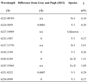
Table 2: Absolute wavelengths of non- Fe I lines. ... 65

Table 3: Mean radial velocities. Errors include seasonal scatter and measurement errors. .. 82

Table 4: Comparison of Orbital solutions ... 86

Table 5: Photometric periods between 1000 and 2000 days ... 92

Table 6: Photometric periods between 100 and 200 days ... 96

Table 7: Photospheric velocity spans and mass-loss rates ...119

Table 8: Observational details of Antares and Betelgeuse ...122

(10)

ix

List of Figures

Figure 1: Hertzsprung-Russell diagram. ... 2

Figure 2: Hertzsprung-Russell diagram showing the regions of hot, cool and coronal winds. 8

Figure 3: Power spectra of one Mira (R Leo) and two semiregular variables. ... 16

Figure 4: Smoothed power density spectra in log-log representation. ... 17

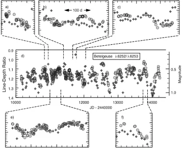
Figure 5: Line-depth ratio plotted as a function of time and AAVSO brightness estimates

binned in 10 day intervals for Betelgeuse. ... 20

Figure 6: WHT and COAST near-infrared interferometric observations of Betelgeuse ... 23

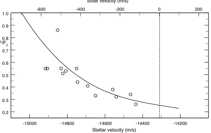
Figure 7: Line-depth ratio (temperature) is plotted as a function of mean core velocity for

Betelgeuse. ... 25

Figure 8: Top – Schematic diagram of a large star spot showing different epochs of stellar

rotation. Bottom – Sample graphs of the luminosity and the stellar radial velocity that

coincide with each epoch. ... 29

Figure 9: Hipparcos light curve of a classical Cepheid using data from Perryman (1997).

(Aerts et al. 2010) ... 33

Figure 10: Radial motions of the l=3 octupole modes. (Fig 1.4 Aerts et al. 2010). ... 34

Figure 11: Amplitudes of the radial eigenfunction (FIG 3 Demarque & Guenther 1999). ... 36

Figure 12: The power spectrum of the solar five-minute oscillation.. ... 37

Figure 13: A sketch of the spectrum of Betelgeuse (α Ori) from Secchi (1866). ... 38

Figure 14: Left – schematic of the 1.2 m telescope of the Elginfield Observatory. Right –

picture of the 1.2 m telescope of the Elginfield Observatory. ... 40

(11)

x

Figure 16: Spectrum of the M1.5 supergiant Antares ... 42

Figure 17: Telluric spectrum. ... 44

Figure 18: Cleaning of a cosmic ray hit by the R9 reduction software ... 47

Figure 19: A typical normalization window.. ... 49

Figure 20: ELODIE spectra of the M-supergiant Betelgeuse (upper) and the B-dwarf Regulus (lower).. ... 52

Figure 21: An image of granulation on the solar surface ... 54

Figure 22: A schematic of granular motions ... 56

Figure 23: Left - Correlation between Doppler shift and line flux of the hot and cool plasma results in an asymmetric spectral line. Right - Asymmetry is more obvious when viewing the bisector of the spectral line. ... 57

Figure 24: This sample of bisectors demonstrates the changes of asymmetry with spectral type in cool stars. ... 59

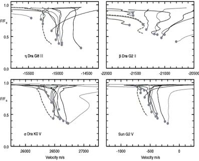
Figure 25: Sample of four third-signature plots.. ... 60

Figure 26: Six Fe I line bisectors computed from the mean lines of five exposures of α Ari. Core positions are marked with circles. The typical error on core position is <50 m/s. ... 63

Figure 27: Bisector core points (circles) from Figure 26 plotted over the Universal curve (solid-line) from Gray (2009)... 63

Figure 28: A bisector from a non-Fe I line taken from one of the five exposures. This bisector is assigned a core velocity using its depth on the Universal Curve. ... 64

Figure 29: Final third signature plot including Fe I and non-Fe I lines... 64

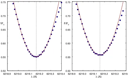
Figure 30: Example of core parabola fitting ... 67

(12)

xi

Figure 32: A sample of the core radial velocities for lines of three different depths. ... 70

Figure 33: Sample of the temporal variations of the line-core flux in the top panel (for the

6241Å line) and the line-depth ratio (6252Å/6253Å) in the bottom panel. ... 71

Figure 34: AAVSO light curve of Antares A the data are binned in 10-day intervals. ... 74

Figure 35: Fourier amplitude spectrum of the 10-day binned AAVSO light curve of Antares

A. ... 75

Figure 36: AAVSO data (as Figure 34) shown with the sinusoid corresponding to the

7140-day timescale ... 76

Figure 37: Power spectrum after prewhitening of the 7140-day variation.. ... 77

Figure 38: Light curve of Antares A. ▲ - Hipparcos & Tycho magnitudes in 1-day bins. ● -

AAVSO magnitude estimates in 10-day bins.. ... 78

Figure 39: AAVSO (●) and Hipparcos (▲) light curves with a 1260-day sinusoid r. ... 79

Figure 40: Radial velocity curve of Antares during 2008-2010... 80

Figure 41: Line-depth ratios (◆) and radial velocities (●) as a function of Julian Day. The

abscissa offset amounts to the minimum temperature occurring 70 days after the minimum in

the radial velocity ... 82

Figure 42: Mean radial velocities phased to a period of 2167 days.. ... 85

Figure 43: Mean radial velocities as a function of orbital phase.. ... 86

Figure 44: Radial velocity (▲) and AAVSO magnitudes (●) means as a function of Julian

Day for three of the four radial velocity data sets.. ... 88

Figure 45: Fourier power spectrum of the AAVSO photometry, prewhitened and focused on

the 1260-day peak.. ... 94

(13)

xii

Figure 47: Residuals of the Smith et al. (1989) are shown by the black points. The grey

curves are 100-day sinusoids. ... 98

Figure 48: Fourier power spectrum of the radial velocity residuals from the data of Smith et

al. (1989). The main peak occurs at 260 days and is flanked by several smaller peaks. ... 99

Figure 49: AAVSO binned magnitude estimates (●) and line-depth ratios (▲) as a function

of Julian Day. ...100

Figure 50: Top – Line-depth ratios measured from 2008 - 2010. Bottom - Hipparcos

magnitudes from 1989-1991 (●) and AAVSO magnitudes over the same epoch (o). ...101

Figure 51: Line-depth ratio residuals as a function of radial velocity residuals for individual

seasons.. ...102

Figure 52: Left - Mean residual velocities from 2009 as a function of Julian Day. Right –

Mean residual velocities from the three strongest lines in the spectrum of Antares. ...105

Figure 53: Top - Season mean third-signatures. Bottom – Mean third signature constructed

by averaging the core position of lines with similar strengths.. ...106

Figure 54:Residual third-signature plots...109

Figure 55: Telluric lines seen in the spectrum of Antares. ...111

Figure 56: Spectral lines shifted to negate the radial velocity shifts and scaled to ensure that

the 6253Å line is the same depth in all lines...112

Figure 57: A 7Å window showing two spectra from 2008, 2009, and 2010. ...114

Figure 58: A 5Å window showing two spectra from 2008, 2009 and 2010. The dashed line

shows the result of convolving the 2008 data with a gaussian with a width of 650 m/s. ...115

Figure 59: Third signature of Betelgeuse...117

(14)

xiii

Figure 61: A section of the HR diagram from Figure 1. The symbol size represents the

(15)

xiv

List of Appendices

Appendix A: The Richardson Image Slicer ...150

Appendix B: Fourier Analysis of Spectral Lines ...152

(16)

Chapter 1

1

Red Giants and Supergiants

Red giants and red supergiants are two related groups of stars, both are in the latter stages

of their evolution. Figure 1 shows the position of these stars on a Hertzsprung-Russell

(HR) diagram. Both groups contain stars cooler than ~5,000˚K, or K and M spectral

class stars, but the members differ greatly in their respective radii and luminosities. Stars

within both groups are much larger and much brighter than a main-sequence star of the

same mass. The red supergiants fall into luminosity classes Iab-II and the red giants into

class III.

Due to the variability demonstrated by essentially all evolved stars, these stars have been

collectively termed the red variables – a title that does little to suggest the nature or origin

of the variations. They have also been referred to as long period variables owing to the

fact that they are variable and have periods considerable longer than most hot stars. As

the light variations of these stars were more extensively studied, three classifications of

variability were established: Mira type, semiregular and irregular. More recent studies

(Kiss & Percy 2012 and references therein) have blurred the boundaries between these

groups. Further details regarding the classifications and the variable nature of these stars

will follow.

Many of the attributes of these stars arise due their advanced state of evolution, thus the

evolutionary history of stars in the upper right of the HR diagram is vital to our

understanding. Unfortunately, stellar evolutionary models are fraught with

simplifications and inconsistencies with observations. Despite this one sees

commonalities in the predictions made by the models; thus, we have some general sense

of how stars evolve after the main sequence. These changes are reviewed in the

(17)

Figure 1: Hertzsprung-Russell diagram. The heavy line indicates the zero-age main

sequence. Points from two evolutionary models are shown as black dots (data from

Paczynski 1970) with connecting grey lines approximating the evolutionary tracks. The

1 M⊙ track is truncated at the helium flash (full evolutionary details follow). The

region of classical pulsational instability is enclosed by the two dashed lines

(approximated from Figure 5.11 LeBlanc 2010). The gray region encompasses the

domain of the red variables and incorporates both red giants and red supergiants

(18)

1.1 Evolution History

In order to understand the nature of red giant and supergiant stars, one needs to

understand their origin and their evolutionary history. Red variables are in the late stages

of stellar evolution which can result in complicated internal structure. The offset and

onset of various core fusion processes results in fusion taking place in shells above the

core (for further details see the sections that follow). This arrangement is pulsationally

and thermally unstable; a number of variable phenomena are associated with such shells,

for example pulsation in Mira-variables (Ulmschneider 1998) and thermal pulses during

very advanced stages of evolution (Aerts et al. 2010). Additionally, the depth of the

outer-most shell will limit the depth of the convective envelope, since this shell will

move outward over time the scale of convection will change for stars at different stages

of their evolution (Kippenhaun & Wiegert 1994). Most importantly it is the highly

evolved states of these stars that results in their large radii, large luminosities and low

surface gravities: when considering the physics underlying their variability these factors

must be kept in consideration. In the following sections we will review the details of

stellar evolutionary models for stars of various masses that ultimately result in red giants

and red supergiant stars.

In Figure 1 the zero-age main sequence is indicated by the heavy line, two evolutionary

tracks are shown originating at the main-sequence and tracking rightward and/or

vertically across the Hertzsprung-Russell (HR) diagram. The almost vertical branches of

these evolutionary tracks are the Red Giant Branch (RGB) and the Asymptotic Giant

Branch (AGB). During their evolutionary progression across the HR diagram all but the

most and least massive stars (0.5M⊙<M_<10-15M⊙) will spend some time on one or

both of the giant branches.

Let us consider a typical star: it will begin its life on the main-sequence, fusing hydrogen

at its core. During its main-sequence lifetime it will evolve slowly due to the build-up of

helium in the core. As the abundance of helium within the core increases we eventually

reach a point where the core is considered hydrogen deficient. Hydrogen deficiency

(19)

M-dwarf(Hansen & Kawaler 1994). From this point on the evolution is considerably

different for stars of differing mass; thus we consider three groups, stars with a mass

greater than 10-15M⊙, stars with a mass between ~3M⊙ and ~10M⊙, andstars with mass

less than ~3M⊙. [Most values given here are taken from Kippenhaun & Wiegert (1994),

and while typical are by no means absolute, see Iben (1974) for other examples].

1.1.1 Intermediate Mass Stars (2.5M

⊙

to 10M

⊙

)

When the stellar core is too deficient in hydrogen to continue fusing, the star has an inert

helium core surrounded by a hydrogen-rich shell that is fusing hydrogen at its base (Ryan

& Norton 2010). The increase in molecular mass, resulting from the hydrogen fusion

above the core causes the core to contract. Energy released by this contraction prevents

the core from becoming isothermal and the low initial central density means that the

contraction is insufficient to cause degeneracy. The core heats and eventually helium is

ignited. This entire period lasts only ~105 years, during which time the stellar radius

increases by ~25 times. These stars have reached the red-giant region of the HR diagram,

a star climbs the RGB before settling into stable core helium burning for ~107 years,

during this period the star moves slowly leftward on the HR diagram until the core

helium content is ~25% when it moves rightward again.

This phase in stellar evolution is crucial in explaining the existence of the classical δ

Cephei type variables. The first crossing of the HR diagram occurs during helium core

collapse, this phase is very short and we are thus unlikely to see stars during this crossing,

this leads to the well-known Hertzsprung gap. Thus, the evolutionary loops account for

the occurrence of these yellow (spectral class G-K) giants and bright giants.

Evolutionary models, like those shown in Figure 1, place a lower mass estimate on the

Cepheid variables of ~5M⊙(Wallerstein 2002).

The extent of the loops depends upon the stellar mass, for stars lower than ~5M⊙ there is

essentially no loop and the star first ascends and then descends the RGB before ascending

(20)

into an ‘ash’ of carbon, oxygen and neon. Helium burning continues, in a shell around

this core, as this shell burns outward the core accretes mass. The hydrogen burning shell

is extinguished due to its temperature falling as it moves outward through the star. With

this shell extinguished the outer envelope expends dramatically and the stellar luminosity

increases strongly, a counterintuitive result caused by the interaction between the two

fusing shells (Kippenhaun & Wiegert 1994). Eventually, the combination of the outward

progression of the helium burning shell and the deepening of the lower convection

boundary results in the re-ignition of the hydrogen burning shell.

Further loops are possible for stars with sufficient mass in which internal contraction will

raise the temperature enough to allow ignition of heavier elements. Each successive loop

will have successively shorter life-time and each will return the star to the AGB. If the

core becomes degenerate before the next ignition temperature is reached then the star

may undergo a carbon, oxygen, silicon or neon flash (see below for details regarding the

helium flash and post flash evolution) before settling on the AGB and forming a heavy

white dwarf. Further evolution, beyond the AGB. is beyond the scope of this work but

details may be found in Kippenhaun & Wiegert (1994).

While on the AGB most stars will become pulsationally unstable and will undergo large

amplitude radial pulsation. Many red variables stem from these stars during their ascent

of the AGB, Miras and some types semiregular variables belong to this evolutionary

group. It is not uncommon for Mira variables in the late stages of AGB evolution to have

emission lines in their spectra. These emission lines arise due to atmospheric heating

caused by the shocks that result from the interaction of pulsation and convection (Freytag

& Hoefner 2008).

1.1.2 Low Mass Stars (0.5M

⊙

to 2.3M

⊙

)

The evolution of low mass stars is quite different than the evolution outlined above for

intermediate mass stars, for such stars degeneracy becomes important. In these stars the

(21)

do see stars in this phase. The energy produced in the hydrogen burning shell causes the

outer layers of the star to expand, the star is limited in its redward progression (or

cooling) and thus the expansion is instead accompanied by a huge increase in luminosity,

often by as much as a factor of 100. As the star climbs the RGB the core continues to

contract and eventually the temperature is sufficient to ignite helium fusion.

The degeneracy of the stellar core has an important effect, termed the Helium flash.

Degeneracy pressure supports the core and the star experiences nuclear runaway: the core

temperature increases rapidly while the central density remains constant. As the central

temperature continues to increase the degeneracy is lifted and thermal pressure begins to

dominate the core. The core can now cool to ‘normal’ helium fusing temperatures and

settles into stable helium burning on the horizontal branch. While on the horizontal

branch the hydrogen burning shell deposits helium onto the helium burning core. During

this phase of evolution some of the stars will cross into the instability strip, these are the

W Virginis stars (Wallerstein 2002). Helium is consumed in the core and carbon and

oxygen are produced. In the same way that the build-up of a central helium ‘ash’ ended

the main-sequence, now a build-up of a carbon-oxygen ‘ash’ ends the horizontal branch.

Nuclear burning now takes place in two shells, the star approaches its Hayashi limit and

begins to climb the AGB. As the star climbs the AGB the two shells burn outward, the

hydrogen shell ceases burning and later begins again as it is heated from below by the

encroaching helium burning shell. The star continues to expand and has a white dwarf

slowly forming at its core.

The stars considered in this thesis are of higher mass than the stars in this group, though

these low mass stars do ascend the HR diagram resulting in AGB stars. Many red

variables (Mira variables and M-giant semi regular variables) are evolved, AGB stars of

(22)

1.1.3 High Mass Stars (>10M

⊙

-15M

⊙

)

In this regime we run into the problem that theoretical evolutionary models have

experienced a lot of difficulty in explaining the observed positions of stars on the HR

diagram. The extreme mass-loss rates these stars experience at the various stages of their

evolution (Massey 2003) makes modeling difficult, combine this with uncertainties

surrounding core convection and interior mixing and the difficulty becomes extreme.

Similar to the less massive stars they will inevitable reach a state of hydrogen deficiency

in their cores, leading to hydrogen shell burning and a shifting of the convective zone.

As before the helium build up in the inert core causes the temperature to rise until helium

burning begins, as for intermediate mass stars this is a short evolutionary phase. Due to

the nature of the processes in these stars, which are as of yet not fully understood, only

the least massive (that is 15M⊙-40M⊙) ever become red supergiants (Humphreys &

Davidson 1979). For details regarding the evolution of the extremely massive stars see

Meynet et al. (2011) and Maeder & Meynet (2012).

The red supergiant phase is relatively short (~100,000 years) and thesestars will

eventually either explode as hydrogen-rich supernovae or, due to their substantial

mass-loss, evolve blueward once more giving rise to yellow hypergiants, high-mass cepheids,

blue supergiants, Wolf-Rayet stars, and/or luminous blue variables. Some of these stars

will return briefly to the red supergiant phase before their dramatic climax (Smartt et al.

2008), while others will result in their supernovae while still in their hot blue phases

(Meynet et al. 2011). Rarely, the most massive red supergiants will later result in the

least massive Wolf-Rayet stars.

The star that is the primary consideration of this thesis, Antares A and its close

comparison star Betelgeuse are both red supergiants. The importance of stellar evolution

lays in this fact, since the similarities and differences between Antares, Betelgeuse and

other red variables could trace their physical origins back to their internal differences due

(23)

1.2 Stellar Winds in the Upper HR Diagram

For many red giants and supergiants mass-loss rates are extreme (~10-6 M⊙ yr-1; de Jager

et al. 1988) and each stage of their evolution is governed by this mass-loss, further the

total mass lost during any one part of their evolution affects their advancement through

the following stage (Mauron & Josselin 2011). Also, RGB stars, AGB stars and red

supergiants all undergo mass-loss, however a well-understood mechanism exists only for

dusty variables (i.e. Mira variables and OH/IR stars). The interaction, if any, between

Figure 2: Hertzsprung-Russell diagram showing the regions of hot, cool and

coronal winds. The line separating coronal winds from cool winds is known as

the Linsky & Haisch dividing line, it occurs at approximately spectral class K1

(24)

stellar winds and photospheric dynamics is not fully understood. All of the proposed

mechanisms of wind driving in red variables (outlined below) should cause a dynamical

effect in the photosphere. If, for example, they are pulsationally driven then the pulsation

velocity will be detectable in the photosperic dynamics even though the wind itself does

not originate there. As observers we should be aware of the expected mechanisms as

much as theoreticians should be aware of the measured velocity scales.

In the upper portion of the HR diagram two types of wind dominate the observations: hot

winds and cool winds. Figure 2 shows the Linksy & Haisch (1979) dividing line, which

separates hot winds from cool winds on the HR diagram. In this figure coronal winds are

also includedand though some evolved stars are found to have corona those under

consideration here do not. Betelgeuse (α Ori) can be seen in the upper-right of Figure 2

and Antares falls in approximately the same location on the HR diagram. Stars hotter

than spectral-type B3 (on the main-sequence this translates to M>6 M⊙) undergo

significant mass-loss due to their high-velocity winds. In these stars, radiation pressure

from mid-UV photons on high-opacity metal lines above the photosphere dominates the

momentum (Castor et al. 1975).

Winds in cool-evolved stars have been measured since the second half of the 20th century

(Deutsch 1956). The winds of these stars are low velocity (20-50 km/s) but still cause

considerable mass-loss, at present no single mechanism successfully explains the

observations (Judge & Stencel 1991, Bennett 2010). Mass-loss rates vary across the

upper HR diagram: line-driven hot winds reach their maximum for hot O stars and cool

winds reach their maximum in the extremely cool red supergiants (see the data presented

by de Jager et al. 1988 or more recently Figure 8 of Cranmer & Saar 2011). The lowest

mass-loss rates occur between late A and early G spectral types. However, due to

differences in evolutionary age, initial mass, mutliplicity and so on, the actual cut-off

from one regime to another is not well defined. Additionally, both high-mass stars and

AGB stars undergo mass-loss events via ejection. Luminous blue variables (or S Dor

stars) are known to undergo massive ejection events throughout their lifetimes, such as

the 19th Century eruption of η Carina discussed by Rest et al. (2012). Mira variables are

(25)

(Etoka & Le Squeren 1997). Photometric flare events of order tenths of magnitudes

(Mais et al. 2004) have also been reported for several dozen Mira variables.

1.2.1 Driving Mechanisms

It is widely accepted that the winds of hot stars are driven by UV-photon momentum

transfer to high opacity metal lines (Castor et al. 1975). For cool stars, coronal winds are

thought to be driven by Alfvén waves (Cranmer & Saar 2011), whereas no single

mechanism is accepted as the cause of noncoronal winds. Some success has been had in

modeling the dusty winds of Miras and OH/IR stars (Bowen 1988; Bowen & Willson

1991) but for dust-free corona-free stars there is still no real consensus. It remains useful

to review the findings for Miras, since they represent a close evolutionary analogue to the

semiregular variables, and to discuss the other possible driving mechanisms.

Dust Opacity - radiation pressure on the dust grains around red giants and supergiants

has been popular as a proposed mechanism for the large winds that these stars

demonstrate (Hofner 2008). Dust grain opacity peaks in the infrared, the same region as

the stellar spectrum, strengthening the argument. However, both dust-free AGB & RGB

stars and the majority of red supergiants have low opacity winds. Further, in those

supergiants where dust is detected it is generally beyond the wind radius: Bester et al.

(1996) report a dust shell around Betelgeuse (α Orionis; M2Iab) at a distance of ~30R∗,

which lies well beyond the wind radius found empirically by Harper et al. (2001).

Although dust opacity is often cited as the cause of strong winds around Miras, OH/IR

stars and other dusty AGB stars, modeling suggests that while the dust facilitates the

mass-loss it is initiated by pulsation lifting the stellar atmosphere (Bowen 1988; Bowen

& Willson 1991).

Pulsation – as mentioned above, pulsation as a mechanism for material to escape the

stellar gravitational potential has been successful in modeling the winds of Mira

variables. In these stars the mass-loss is augmented further by radiation pressure on dust

(26)

mass-loss rates for stars when the pressure-scale heights became large, even in the regime of no

dust. Thus, we see that if the surface gravity is low then strong winds can develop. It has

been argued that the smaller pulsation amplitudes in red supergiants make this simulation

implausible (e.g Josselin & Plez 2007).

Alfvén Waves - magnetic waves have been proposed as a choromospheric heating

mechanism and thus an energy transfer mechanism for these cool wind stars (Schroder &

Cuntz, 2007) due to their large damping lengths. However, these waves couple to

ionized gas, whereas the cool winds of K and M supergiants are neutral. Thus,

momentum and energy transfer via this mechanism would be extremely inefficient.

Acoustic Waves - convection in cool stars drives atmospheric turbulence and acoustic

waves, some of which will penetrate the higher atmospheric layers. On the whole models

show that while short period acoustic waves in the Sun can efficiently heat the

chromosphere they are unlikely to drive the stellar winds (Athay & White 1978;

Hartmann & MacGregor 1980; Cuntz 1990). However, the nature of convection in red

supergiant stars is quite extreme (Gray 2008 amongst others) and, although short period

acoustic waves may not be sufficient to drive their winds the thermal and kinetic energy

imparted on the atmosphere by the convection cells directly likely has a much larger

impact.

1.3 The Red Variables

As was previously mentioned, at various points throughout a stars evolution it may

experience times of variability. During horizontal branch evolution some low-mass stars

will cross into the instability strip, these are observed as either RR Lyrae variables (for

further reading see Smith 1995) or W Virginis stars (for further reading see Wallerstein

2002). Similarly, the evolutionary looping of intermediate mass stars causes them to pass

through the instability strip, giving rise to the classical Cepheid variables (see Wallerstein

2002). It is however the red variables that are of interest to this thesis. Unfortunately,

(27)

metallicity and so on) are wildly different and thus assigning an evolutionary phase to

any individual red giant or red supergiant is not trivial. Instead when considering these

stars we consider these stars in terms of the nature of their variability.

Long period variable stars are stars in which brightness variations occur over many

months or years, here we use this term in its broadest sense, that is in referring to all

luminous red variables, however some literature uses this term to apply to the

Mira-variables only. Typically these stars are of luminosity class III or brighter, and of

spectral class F and cooler. The General Catalogue of Variable Stars (GCVS, Samus et

al. 2012) lists three categories of red variables: Mira variables (M), Semi-regular

variables (SR), and Slow Irregular variables (L). These classifications are discussed

below.

Mira Variables – The GCVS (Samus et al. 2012) gives three distinguishing

characteristics for these stars: Their periods are typically between 80 and 1,000 days.

They are of spectral types Me, Ce, or Se indicating low effective temperature and

emission features, likely from atmospheric shocks typical of the later stages of AGB

evolution. The amplitudes of their light curves fall between 2.5 to 11 mag in V, though

the bolometric magnitude variation is ~1 mag (Willson & Marengo 2012). Thus the

bolometric luminosities increase by approximately a factor of 2. The large optical

amplitudes arise from large variations in the opacity over a pulsation cycle. These stars

are late-AGB stars typically of low mass (<2M⨀), they are radial pulsators, however,

identifying the mode of pulsation, that is fundamental mode or overtone pulsation, of

these variables has been difficult (Wood 1995 gives details pertaining to is problem and

reviews the observational and theoretical evidence). Fundamental mode pulsation is

favoured.

Semiregular Variables – In the GCVS (Samus et al. 2012) this class of stars

encompasses several group of stars and thus is further classified. However, they all

display some common features: they are giants and supergiants that are of

intermediate-to-late spectral-types, and demonstrate notable variability. These stars are subcategorized

(28)

SRa – these stars are small amplitude Mira variables, as such they have periods that

are fall into the same range as those of Mira variables but have visual magnitudes

<2.5 mag. The classification of these stars as semiregular variables rather than Miras

seems to be based solely on their visual amplitudes (Kerschbaum & Hron 1992).

SRb – SRb stars are also evolved giants but have smaller amplitudes than SRa stars

and poorly defined periods, typically between 20 and 2300 days. These stars often

vary between periodic and irregular and in some cases are multiperiodic.

SRc – these are small amplitude (<1 mag), semi-periodic evolved supergiants with

periods similar to those of SRa and SRb variables.

SRd – these are weak-lined, F, G, and K giants and supergiants. They are considered

to be a metal poor, short period analogues (<1100 days) of Miras (Lloyd Evans

1975). They have visual amplitude of ≤4 mag.

These categories seem somewhat arbitrary, being based solely on the amplitude of the

variation and the spectral and/or luminosity classification. Only two of these

classifications appear to be truly semiregular with the other two falling into this group

based solely on them being not Miras. The group of importance to this thesis is the SRc

variables which is mostly comprised of M class supergiants; in fact the well-studied

supergiant Betelegeuse is classified as an SRc variable.

Slow Irregular Variables – These stars have light curves that are highly chaotic and that

show little to no periodicity. Similar to the semiregulars these stars are further grouped

depending on their luminosity class: Lb designating the giants and Lc designating the

supergiants. Many stars within this group are classified as such simply due to lack of

observation, thus the true nature of the variability is not known and many are likely

semi-regular stars with few observations. Antares A is classified as an Lc variable in the

(29)

Chapter 2

2

Observations of Semiregular and Irregular Variables

Despite their differing classification, semiregular and irregular variables share many

physical traits and thus in this section we will consider these stars simultaneously. Here

we will see how many of the observed features of these stars cannot be satisfactorily

explained by radial pulsation. A star becomes known as a variable if its apparent

brightness changes over time, with most stars displaying at least some variability. ο Ceti

(Mira) was the first star for which variability was recorded, in 1596 Fabricius noted the

appearance and disappearance of this star while monitoring Mercury. This was followed

by the discovery of, the S Dor variable, P Cygni in 1600. In the following 200 years a

further 13 variable stars where recorded, 8 of these 15 are now considered red variables

by spectral type. The most recent edition of the GCVS (Samus et al. 2012) lists >40,000

variable stars in the Milky Way, the majority of which are red variables.

2.1 Photometry

Light curve analysis has been the principal method for period estimation in these stars for

more than 50 years (e.g. Payne-Gaposchkin 1954, Fredrick 1960a & 1960b, Stothers &

Leung 1971) and such photometry has played a critical role in our understanding of red

variables. Detailed studies of the light curves of red variables have shown some

interesting results: Mira-variables have regular, periodic lightcurves, but even the

cleanest examples have some irregularity superimposed. Similarly, semiregular variables

appear mostly irregular although a characteristic timescale of variation can be identified

(Mattei 1983).

For a convincing physical interpretation of the variability to be made, quality

observational material is required. As stated above, the light changes in these red

variables typically occur with periods between 20 and several thousand days. In the case

(30)

Such long timescales make it difficult to obtain well-sampled light curves, this is

especially problematic for semiregular and irregular variables which demonstrate erratic

variations. Hence, only a small number of good, long and well-sampled light curves have

been published, and in the past many of the published pulsation parameters were

questionable, an issue highlighted by Lebzelter et al. (1995). However, in recent years,

visual magnitude estimates made by amateur astronomers have been made available

electronically through archives such as that maintained by the American Association of

Variable Star Observers (AAVSO). While the quality of individual measurements within

the database is low,the power of this data lies in its unprecedented coverage (see Percy &

Mattei 1993). In fact, several studies of red variables are based on such data (e.g. Mattei

et al. 1997; Kiss et al. 1999, 2000, 2006). In Chapter 6 we present the AAVSO light

curve of Antares and use these data to study the photometric variations.

2.1.1 Photometric Power Spectra

Fourier power/amplitude spectra of time variable data provide a wealth of information

about the nature of the variability. The peak positions tell us directly the frequency of

any oscillation and the sharpness gives information about the phase stability and/or the

duration of the observations. Stars undergoing regular, radial pulsations have sharp

peaks, like that of the Mira variable R Leo (Bedding 2003) shown in the upper panel of

Figure 3. In the past decade, numerous examples of photometric periodograms have

shown (see the lower two panels of Figure 3 for example) that peaks in the power spectra

of semiregular variables closely resemble the power peaks associated with the solar

5-minute oscillation (Bedding et al. 2003, Kiss et al. 2006). Such similarity is suggestive

of a similarity in the underlying mechanism, that is convection (or granulation) driven

variations. With the new era of high precision photometry, from telescopes such as

MOST, KEPLER, and CoRoT, 1000s of red giants have been identified as demonstrating

(31)

Figure 3: Power spectra of one Mira (R Leo) and two semiregular variables. The

plots demonstrate the differences between the power peaks of an opacity-driven

radial pulsation compared to stochastically driven oscillations. The inset panels show

(32)

(33)

The physical nature of the variations can also be investigated through studying the shape

of the power density spectrum. The analysis of fluctuations in power density spectra is a

common tool in studies of unpredictable and seemingly aperiodic variability, that is,

noise that arises from stochastic processes. In this context, the noise is intrinsic to the

source and not a result of measurement error. Kiss et al. (2006) studied the power

density spectra of a number of red variables. Figure 4 shows the close similarity in the

log-log slope; Kiss and collaborators concluded that there is a universal scaling behavior

in the brightness fluctuations. Yet again these results are similar to results found for the

solar-granulation background (Rabello-Soares et al. 1997) and are even expected to arise

from convection. For further details of the phenomenon of 1/f noise the reader is directed

to the papers of Bak et al. (1988) and Press (1978).

2.1.2 Long Secondary Periods and Multiperiodicity

Long secondary periods are seen in the light curves of many semiregular variable stars

(Houk 1963) these periods are of the order 500-2000 days (some 5-15 times the primary

period). In the Large Magellanic Cloud (LMC) some 25% of semiregular variables have

been found to show such periods (Wood et al. 1999). Multiperiodicity has also been

reported in a number of investigations (e.g. Kiss et al. 1999) suggesting that the visual

light changes may be described with the coupling of two or three excited periods. The

use of the Fourier amplitude spectra allows for the selection of many periods, and this can

improve the fit of the light curves. However, a physical explanation for a large number

of periods seems unlikely. The very longest periods found are unlikely to be due to

pulsation (see Wood 2000), however the shorter periods could represent different modes

of pulsation. To-date no single mechanism has been accepted as the cause of

multiperiodicity, though a number of suggested causes are to be found in the literature:

the possible explanations include orbital dynamics, radial pulsation, rotation combined

with surface irregularities, and episodic dust ejection. In recent years non-radial

pulsation has gained more support than the other proposals (Olivier & Wood 2003),

though it is also suggested that an as yet unknown pulsation mechanism is required to

(34)

had success in explaining an observed long secondary period – in particular for the RVb

type variables (RV Tauri stars with long secondary periods) it is binarity that produces

the long secondary period (Maas et al. 2002 and Van Winkle et al. 1999 amongst others).

2.1.3 Period-Luminosity Relations and Mode of Pulsation

Interest in semiregular variables was driven by the hunt for a period-luminosity relations

similar to those seen for classical Cepheids and Mira variables. The large intrinsic

brightness of semiregular variables makes them desirable as distance indicators. Wood et

al. (1999) presented five different period-luminosity sequences for the LMC red variables

based on the MACHO photometric database and they found that the third and even forth

overtones could be the dominant excited modes. A detailed review given by Percy &

Parkes (1998) draws similar conclusions. Following the results shown for LMC red

variablesKiss et al. (2006) investigated the long secondary period phenomenon in a

selection of red supergiant stars including Antares and Betelgeuse. The work of Kiss and

collaborators suggests that galactic red supergiants may follow period-luminosity

relations that are an extension of those seen for less luminous red variables in the LMC.

In this case one sees, usually, two period-luminosity relations one for a short (or primary)

period of radial pulsation (~300-400 days) and one for the long secondary period (≥1000

days).

Further, Bedding et al. (1998) reportedly observed mode switching in R Dor and claim

that it occurs between the first and third overtones. Mode switching has been reported in

other semi-regular variable stars (Cadmus et al. 1991; Percy & Desjardins 1996; Kiss et

al. 2000) and in conjunction with multiperiodicity (Kiss et al. 1999; Percy et al. 2001)

and the studies of semi-regular variables in the Magellanic Clouds (Wood et al. 1999;

Wood 2000) the idea that the light variations seen in semi-regular variables may be due

to many simultaneously excited modes seems increasingly attractive. However, the mode

of pulsation of these stars is still a matter of some debate and even the cleanest examples

of multiple period semi-regulars exhibit additional irregularity in their light curves

(35)

stationary frequency and amplitude content cannot fully explain the light variations that

are observed.

2.2 Temperature Variations

Radial pulsation shows a ratio between the light variation and the color variation that is a

constant function for any given star. However, in a selection of AGB stars Kerschbaum

et al. (2001) found some light phases to be accompanied by strong color changes while

Figure 5: Line-depth ratio plotted as a function of time () and AAVSO

brightness estimates binned in 10 day intervals (+) for Betelgeuse.

Temperature and brightness maxima often agree but occasionally there is

(36)

others showed very little variation. Interpreting the color value as an indication of the

temperature, this implies that light change is observed even during times of constant

temperature. Additionally, by comparing the line-depth ratio (temperature index, see

Gray & Brown 2001) and brightness variations over the same period, Gray (2008) found

that the temperature variations of Betelgeuse did not account for all the observed

brightness variation, see Figure 5. These observations suggest that radial pulsation alone

cannot account for the observed variation of the brightness of these stars.

2.3 Radial Velocity

Studies of short-term (~200 days) radial velocity variability in semiregular variables

(Lebzelter et al. 2000; Lebzelter & Hinkle 2002) show radial velocity curves with

minima that occur very near maximum light, a behavior typical of radial pulsators (see

for example. Bersier et al. 1994a, 1994b). This suggests that the light variations are

dominated by radial pulsations. However, “jitter”, or excess irregularity in the

radial-velocities of stars at the tip of the red giant branch has been seen repeatedly (Gunn &

Griffin 1979; Pryor et al. 1988; Carney et al. 2003, among others). Many of these studies

have found jitter to be concentrated to the most luminous of the target stars. Currently,

the leading candidates for the cause of the jitter are: (i) some form of modulation (see

Carney et al. 2003) added to the photometric variability, and (ii) giant convective cells

(Gray et al. 2008; Eaton et al. 2008). The idea of time-variable dark or bright regions

seems probable in either case.

2.4 Interferometry

Hot/bright spots on the surfaces of a handful of M-type supergiants have been seen in

interferometric studies for many years (Buscher et al. 1990; Wilson et al. 1992; Tuthill et

al. 1997; Young et al. 2000). However, the cause of these hotspots has been the source

of some conjecture with various suggestions of their origin being made: including the

(37)

non-radial pulsation, and transient convective cells on the stellar surface. Studies of the

evolution of these features gives insight into the physical mechanisms behind them, as

well as some of the other variable features of such stars. Freytag et al. (2002) presented a

short overview of observations of such hotspots (data for the figure taken from Buscher et

al. 1990; Wilson et al. 1992; Tuthill et al. 1997; Wilson et al. 1997; Klueckers et al.

1997; Burns et al. 1997; Young et al. 2000), as seen in Figure 6.

The figure produced by Freytag et al. (2002) shows quite clearly the evolution of these

bright spots as well as their often multiple nature. Changes in spot number and position

are observed on timescales of years; such evolutionary timescales should not be expected

for a multiple system. For example, take VV Cephei a well known red supergiant with a

hot companion star: a system with a period of 7430 days (or approximately 20 years).

Thus, hotspots due to companion transits seem unlikely for similarly large stars.

However, interactions of the primary star with companions cannot be ruled out as

chromospheric heating is known to occur in binary systems (e.g. Eaton et al. 2008).

Similarly, rapid spot evolution also makes a rotational mechanism seem highly unlikely.

Again if we consider an example, derived rotation velocities for Betelgeuse are typically

~5km/s (Gray2000 for example) resulting in a rotation period ~20 years. Not all such

stars will have rotational periods this large but, considering conservation of angular

momentum as the star expands during its evolution, any rotation period is expected to be

much larger than the observed hotspot evolution timescales.

Observations, for example Gray (2000), tend to show that hotspot occurrence is

correlated with low overall brightness. Such a phenomenon is difficult to explain until

one considers the results of stellar atmospheric models. Such models of convection in

red supergiants stars show that hotspots on the simulated stellar surface occur

preferentially at the edges of darker features (Freytag et al. 2002; Freytag & Höfner

2008; Chiavassa et al. 2009). They have also shown that the timescales, sizes and

numbers of the observed hotspots can be explained very well using models of giant

(38)

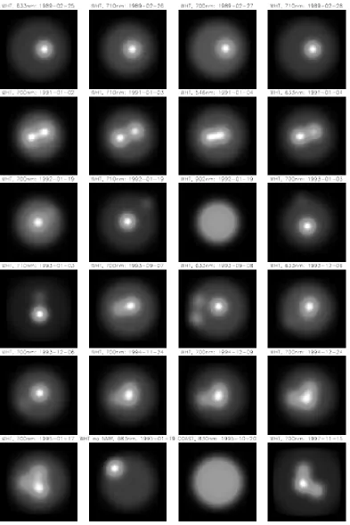
Figure 6: WHT and COAST near-infrared interferometric observations of

Betelgeuse compiled from published data of spot positions and intensities

(39)

2.5 Polarization

Strong circumstantial evidence for localized hotspots on the surfaces of late-type

supergiants has, in the past, come mainly from analyses of polarization observations

(Hayes 1984; Holenstein 1993). The observed polarization of red supergiants is seen to

vary in both strength and direction, suggesting a highly nonspherical physical

mechanism. The observations indicate that at least one characteristic of the star or the

ejected mass must be nonspherical since the polarization is observed to vary in both

strength and direction. Details regarding the source of the polarization, atmospheric

versus dust, may be found in Holenstein (1993). Interestingly the polarization is seen to

vary on time scales similar to the photometric variations.

2.6 Spectral Variability

Observationally the spectral lines of the red supergiant Betelgeuse are seen to vary in

position and depth (Gray 2000; Josselin & Plez 2007; Gray 2008). Despite the variations,

the spectral lines observed in both cases showed only small changes in their widths

suggesting that the macroturbulence is constant. The line core positions are seen to vary

over a range of 9 km/s; such a large shift compared with only small changes in line width,

implies that one bright feature dominates the spectrum. In his concluding remarks, Gray

(2008) suggests that the constant macroturbulence arises from motions within large

atmospheric structures (or convection cells), which as we will see in the next section are

readily predicted from models.

2.7 Photospheric Excursions

Gray (2008) expanded on his observations by plotting the line-depth ratio (the

temperature index) as a function of line-core position (radial velocity), Figure 7. Using

these tools, one easily sees a pattern of heating followed by the material rising, then a

(40)

showing that the more vigorous excursions are hotter, rise faster. The opposite case also

arises where material reaches lower temperatures, rises more slowly, and the excursion

eventually peters out. The relationship seen by Gray (2008) between velocity and

Figure 7: Line-depth ratio (temperature) is plotted as a function of

mean core velocity for Betelgeuse. Each panel encloses a single

observing season. Arrows indicate the direction of increased time. The

characteristic timescale of these variations is ~350 days. Symbol size

indicates measured line-widths (macroturbulence). Panel f) shows a

(41)

temperature varies significantly from the behavior of radially pulsating stars, where

temperature and velocity variations are essentially in phase (e.g. Wesselink 1946;

Walraven et al. 1958). It is easy to imagine how the behavior outlined in Figure 7 would

result from large-scale convection, such behavior coupled with the observed bisector

variations is highly suggestive of large convective cells erupting and sinking through the

(42)

Chapter 3

3

Mechanisms of Variability

As was alluded to in the previous chapter, many physical explanations have been put

forth as the cause of the variability detected in semiregular and irregular variables from

binarity, to rotational modulation, from pulsation to magnetic fields. In this chapter we

review the physical nature and the expected period and magnitudes of these various

mechanisms.

3.1 Companion Stars

It has been well known since the mid-to-early nineteenth century that the majority of stars

occupy multiple systems. It is common practice to classify these systems according to

the method of their observation, many stars are classified in more than one group,

however, the observational techniques are quite different:

Visual Binaries - are binary systems where both stars a readily resolved through visual

telescopic observation. Obviously, resolving power of the instrument directly affects the

number of these stars observed.

Spectroscopic Binaries - these stars demonstrate variations in their radial velocity

(Doppler shifts) as they orbit their combined center of mass. In some cases we may see

spectra of both stars present in the observations, and thus single and double peaked lines

are evident due to the orbit.

Astrometric Binaries - these relatively close stars are seen to wobble around a point in

space. This observed wobble is a result of the orbit around the center of mass, though the

secondary is usual not visible.

Spectrum Binaries - these stars have composite spectra, but either extremely small

changes in their radial velocities or large differences in the spectral types. Thus, we see

(43)

Eclipsing Binaries - the systems appear edge one, thus as one star passes in from of the

other we observe a fall in the combined brightness. These eclipses are seen in light

curves of the system.

For further information on these systems and their classifications see Batten (1973).

Given the preference of stars to form in multiple systems it seems highly likely that many

evolved giants and supergiants, including the red variables, are members of such systems.

In fact, most of the stars that are the focus of this study are known to be such. Thus,

depending on the orientation, contents and dynamics of the system, companion stars can

cause both photometric and radial-velocity variability. In fact, orbital motion has been

suggested by a number of authors as a major contributor toward some of the variability

exhibited by luminous red variables. Orbital motions were proposed to explain the

existence of long secondary periods and muliperiodicity (e.g. Wood et al. 1999, 2004a,

2004b), as well as the interferometrically observed hotspots (Buscher, Baldwin, Warner,

& Haniff, 1990). However, as was discussed in the previous chapter, binary transits are

unlikely to be the cause many of the variable features observed. For example, hotspot

evolution times are too short to be described by transits of a hot companion.

3.2 Surface Features

There are a number of stellar atmospheric phenomena that can cause variations in the

photometry and radial velocity of their host star, as well as other stellar observable

parameters.

3.2.1 Starspots

The movement of surface features on the sun is a well known phenomenon, and

photometric and spectroscopic modulations are attributed to such features in other stars

(Vogt et al. 1987; Vogt 1981 and many others). These features are dark spots on the

(44)

activity within the region of the spot compared to the surrounding area prevents the flow

of energy from the stellar interior by inhibiting convection (Biermann 1938).

Figure 8: Top – Schematic diagram of a large star spot showing different epochs of

stellar rotation. Bottom – Sample graphs of the luminosity and the stellar radial

velocity that coincide with each epoch.

The photometric effects of spots are well documented for late-type dwarf stars (Kron

1947, 1952; Chugainov 1966; Henry et al. 1995). In these cases the light curves appear

modulated with the rotation period of the star and also show small variations due to

inhomogenous spot lifetimes which can vary from a few months to a few years (Bartolini

et al. 1983; Olah et al. 1986; Strassmeier & Bopp 1992; Olah et al. 1997).

Spectroscopically the spots manifest as changes in line-shapes, either the presence of

variable emission humps within absorption lines (in extreme cases) or, more usually, a

variable asymmetry in the spectral lines. Such variability can ultimately cause an

(45)

Combined, one should see maximum luminosity coincident with the mean

radial-velocity, as seen in Figure 8.

Much like companion stars, spots have been identified as the cause of interferometric

hotspots and of the irregular brightness variations of red variables. However the

variations in both cases have timescales much too short to be attributed to a rotational

origin. One must be cautious not to dismiss an argument to hastily, should spot lifetimes

in red giants and supergiants be similar to those of K and M dwarfs, then their lifetimes

would be close to the timescales demonstrated by red variables.

3.2.2 Convection Cells

In 1975 Martin Schwarzschild (Schwarzschild 1975) predicted the existence of

large-scale convective elements dominating the light from evolved giants and supergiants. His

work was driven by the suspicion that convection played a major role in ejection and

mass loss from the atmospheres of these stars. Early scaled solar wind models had failed

to accurately model the circumstellar envelopes of red giant stars (Weymann 1962),

driving the need for a different approach. The first steps were taken by using the

observed diameters of granules and supergranules for the Sun, and through some scaling

assumptions, forming a depth model of their relative positions with respect not only to

one another but also to physical parameters, such as ionization fractions and temperature

of the stellar layers. The models showed that it is possible for the large scale

(supergranulation) to provide the dominant photospheric convection in these stars. His

arguments permitted an extreme picture of convection in red giants and supergiants,

where the dominant convective elements are so large that only a handful of them occupy

the surface of the star at any one time.

The theoretical description of convective motion in the atmospheres of red supergiants

and AGB-stars has made considerable progress since the time of Schwarzschild, thanks

in part to the pioneering hydrodynamic models of solar convection by Nordlund and

(46)

Stein 1999). For examples of models of convection in red giants and supergiants see

Höfner et al. (1998), Höfner (1999), Winters et al. (2000), Freytag et al. (2002), Freytag

(2006), and Chiavassa et al. (2009). Recent modeling has focused on the well-observed

red supergiant Betelgeuse. Most such works agree well with the initial predictions of

Schwarzschild (1975) and while able to recreate the interferometric observations

(Chiavassa et al. 2009) they still struggle to match the spectral observations (Chiavassa et

al. 2006).

Models of large-scale convection in red supergiants typically report large dark and light

areas on the stellar surface. The bright areas are as much as 50 times brighter than the

dark regions (Chiavassa et al. 2010), theoretical images look remarkably similar to

interferometric observations like that of Figure 6. The patterns are highly time variable,

with bright regions having lifetimes of only weeks in the visible. These models suggest

that at these wavelengths the light emerges from high in the atmosphere (τ<1) where the

effects of waves and atmospheric shocks can become important. The interaction of

convection on this scale with other modes of variability is not well understood, though it

is not unlikely that the continual perturbing effect of convective cell emergence drives a

variation (as suggested by Gray 2008 amongst others). Since the rotation rates of red

supergiants are so small any interaction with rotation is unlikely to occur (thus, no stellar

dynamo will be active).

The effect of such large convective cells on the atmospheres allows for some predictions

regarding likely observations. We should expect brightness, temperature, and

radial-velocity changes, however the nature of the envelopes of evolved supergiants and the

stochastic nature of convection mean that the variations will not necessarily be either in

phase or coherent. The cells themselves are expected to vary in size, temperature, and

projection through the atmosphere. These stars are also subject to extreme

limb-darkening, thus the effects of a cell at disk center will be quite different from the effects

of a cell at the limb. In fact, noncoherent and irregular variations are a natural

A Variability Study of the Typical Red Supergiant Antares A

Scholarship@Western

Scholarship@Western

A Variability Study of the Typical Red Supergiant Antares A

A Variability Study of the Typical Red Supergiant Antares A

Abstract

Keywords

Acknowledgments

Table of Contents

List of Tables

List of Figures

Chapter 1

1

Red Giants and Supergiants

1.1 Evolution History

1.1.1

Intermediate Mass Stars (2.5M

to 10M

)

1.1.2

Low Mass Stars (0.5M

to 2.3M

)

1.1.3

High Mass Stars (>10M

-15M

)

1.2 Stellar Winds in the Upper HR Diagram

1.2.1

Driving Mechanisms

1.3 The Red Variables

Chapter 2

2

Observations of Semiregular and Irregular Variables

2.1 Photometry

2.1.1

Photometric Power Spectra

2.1.2

Long Secondary Periods and Multiperiodicity

2.1.3

Period-Luminosity Relations and Mode of Pulsation

2.2 Temperature Variations

2.3 Radial Velocity

2.4 Interferometry

2.5 Polarization

2.6 Spectral Variability

2.7 Photospheric Excursions

Chapter 3

3

Mechanisms of Variability

3.1 Companion Stars

3.2 Surface Features

3.2.1

Starspots

3.2.2

Convection Cells