Estimation of reliability evaluation of Wind Power plant
connected to power grid: An Analysis
Ravi Shankar Garg 1, Anurag Gour2,Dr.Mukesh Pandey 3 1 Mtech Scholar, Energy Technology, RGPV Bhopal, MP, India 2 Asst. Professor. Energy Technology, RGPV Bhopal, MP, India 3
Professor &Head of Department, Energy Technology, RGPV Bhopal, MP, India
Abstract :
The grid was also able to keep up voltage and frequency, and was able to provide any reactive power that was needed. India of 58 numbers of 225 KW each (13.5 MW).The reliabilityevaluation result of 10 units of Dewas plant connected to eastern grid were predictable. The estimates
were based on the performance data of the individual units over a period of one year. The power produced
by the wind turbine increases from zero at the threshold wind speed (cut in speed) (usually around 5m/s
but varies with site) to the maximum at the rated wind speed. Above the rated wind speed, (15 to 25 m/s)
the wind turbine continues to produce the same rated power but at lower efficiency until shut down is
initiated if the wind speed becomes dangerously high, i.e. above 25 to 30m/s (gale force). The exact
specifications for energy capture by the turbine depend on the distribution of wind speed over the year at
the individual site. Air density has a significant effect on wind turbine performance. The power available
in the wind is directly proportional to air density. As air density increases the available power also
increases. Air density is a function of air pressure and temperature. It increases when air pressure
increases or the temperature decreases. Both temperature and pressure decrease with increasing elevation.
Consequently changes in elevation produce a profound effect on the generated power as a result of
changing in the air density.
1. Introduction:
The major sources of electrical energy, in India, are the fossil fuels and water. There are no immediate prospects for large scale utilization of alternate sources of energy like sun, wind, tides etc. for generation of electrical energy. The three types of fossil fuels used in power plants are coal, oil and gas. As it common to know, coal is the predominant source of energy in India and many other countries. Coal contains moisture, carbon, hydrogen, sulphur, nitrogen, oxygen and ash.
The liquid fuels are obtained by refining the crude oil which contains about 84 to 87% carbon, 11 to 16% hydrogen, and oxygen, nitrogen, sulphur etc. Gaseous fuels are either
natural gas or manufactured gas (water gas or producer gas). The manufactured gas is costly and, therefore, not used for power generation. The fuels used in nuclear reactors are natural uranium, lightly enriched uranium dioxide and plutonium.
2. WIND POWER GENERATION
The kinetic energy per unit time, or power, from wind is given by Equation (1). Wind power is proportional to the cube of the wind velocity.
Power of Wind = 1/2 * ρ * A * V3 (1)
Where, P is power in watts, ρ is air density in kg/m3, A is area exposed to the wind (m2), and V is wind speed in m/s.
The actual power production potential of a wind turbine must take into account the fluid mechanics of the flow passing through a power producing rotor, the aerodynamics and efficiency of the combination of rotor and generator. In practice, a maximum of about 45% of the available wind energy is harvested by the best modern wind turbines. Power output from wind turbine can be seen in Equation (2).
Wind Turbine Power Output = 1/2 * ρ * A * Cp * V3 * Ng * N b (2)
where, P is power in watts, ρ is air density in kg/m3, A is area exposed to the wind (m2), V is wind speed in m/s, is performance coefficient (Maximum 0.59), Ng is generator efficiency
(80% on average for grid-connected induction generators), and N b is gearbox and bearings efficiency (Maximum 95%). p
The power produced by a wind turbine can be shown by a power curve. The power curve of a wind turbine is a function that indicates how large the electrical power output will approximately be for the turbine at different wind speeds. The power curve illustrates three important characteristic velocities:
♦ Rated wind speed: the wind speed at which the rated power of a wind turbine, generally the maximum power output of a generator at highest efficiency, is produced.
♦ Cut-in wind speed: the minimum wind speed at which a generator starts delivering power.
♦ Cut-out wind speed: the maximum wind speed at which the turbine is allowed to produce power, usually limited by engineering design and safety constraints. No power will be produced by a wind turbine beyond the cut-out speed.
The power curve of GE 3.6 MW offshore series wind turbine, where rated speed is 14 m/s, cut-in speed is 3.5 m/s and cut-out speed is 27 m/s.
Fig.2 Power Vs Wind speed
A group of wind turbines at the same location are interconnected with a medium voltage power collection system and communication networks, which forms a wind farm. Figure 4.1.2 shows a typical configuration of a wind farm. The power generated from individual turbine are aggregated and delivered to major power systems from the substation at wind farm through transmission systems. A wind farm may be located offshore to take advantage of strong and steady winds blowing over the surface of an ocean or lake.
Fig. 3 Model of Wind Power Plant
3. ASYNCHRONOUS SYSTEM
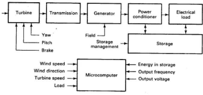
In the previous two chapters, we examined combinations of wind turbines, transmissions, And generators connected to the electrical grid. The electrical grid was assumed to be able to Accept all the power that could be generated from the wind.
The grid was also able to maintain voltage and frequency, and was able to supply any reactive power that was needed. When we disconnect ourselves from the grid, these advantages disappear and we must compensate by adding additional equipment. The wind system design will be different from the synchronous system and will contain additional features.
Block diagram of asynchronous electrical system. In this system, the microcomputer accepts inputs such as wind speed and direction, turbine speed, load requirements, amount of energy in storage, and the voltage and frequency being delivered to the load. The microcomputer
sends signals to the turbine to establish proper yaw (direction control) and blade pitch, and to set the brakes in high winds. It sends signals to the generator to change the output voltage, if the generator has a separate yield. It may turn on on critical loads in times of light winds and it may turn on optional loads in strong winds. It may adjust the power conditioner to change the load voltage and frequency. It may also adjust the storage system to optimize its performance.
It should be mentioned that many wind electric systems have been built which have worked well without a microcomputer. Yaw was controlled by a tail, the blade pitch was exceeding, and the brake was set by hand. The state of charge of the storage batteries would be checked once or twice a day and certain loads would be either used or not used depending on the wind and the state of charge. Such systems have the advantages of simplicity, reliability, and minimum cost, with the disadvantages of regularly requiring human attention and the elimination of more nearly optimum controls which demand a microcomputer to function. The microcomputer and the necessary sensors tend to have a exceed cost regardless of the size of turbine. This cost may equal the cost of a 3-kW turbine and generator, but may only be ten percent of the cost of a 100 kW system. This makes the microcomputer easier to justify for the larger wind turbines.
The asynchronous system has one rather interesting mode of operation that electric utilities do not have. The turbine speed can be controlled by the load rather than by adjusting the turbine. Electric utilities do have some load management capability, but most of their load is
not controllable by the utilities. The utilities therefore adjust the prime mover input (by a valve in a steam line, for example) to follow the variation in load. That is, supply follows demand. In the case of wind turbines, the turbine input power is just the power in the wind
and is not subject to control. Turbine speed still needs to be controlled for optimum performance, and this can be accomplished by an electrical load with the proper characteristics, as we shall see. A microcomputer is not essential to this mode of operation, but does allow more edibility in the choice of load. We can have a system where demand follows supply, an inherently desirable situation.
As mentioned earlier, the variety of equipment in an asynchronous system is almost limitless. The generator may be either ac or dc. A power conditioner may be required to convert the generator output into another form, such as an inverter which produces 60 Hz power from dc.
The electrical load may be a battery, a resistance heater, a pump, a household appliance, or even exotic devices like electrolysis or fertilizer cells. Not every system requires a power conditioner. For example, a dc generator with battery storage may not need a power conditioner if all the desired loads can be operated on dc. It was not uncommon for all household appliances to be 32 V dc or 110 V dc in the 1930s when small asynchronous wind electric systems were common. Such appliances disappeared with the advent of the electrical grid but started reappearing in recreational vehicles in the 1970s, with a 12-V rating. There are no serious technical problems with equipping a house entirely with dc appliances, but costs tend to be higher because of the small demand for such appliances compared with that for conventional ac appliances. An inverter can be used to invert the dc battery voltage to ac if desired.
4. ASYNCHRONOUS (INDUCTION) GENERATORS
Most wind turbines in the world use a so called three phase asynchronous (cage wound) generator, also called an induction generator to generate alternating current. This type of generator is not widely used outside the wind turbine industry, and in small hydropower units, but the world has a lot of experience in dealing with it anyway:
The curious thing about this type of generator is that it was really originally designed as an electric motor. In fact, one third of the world's electricity consumption is used for running induction motors driving machinery in factories, pumps, fans, compressors, elevators, and other applications where you need to convert electrical energy to mechanical energy.
One reason for choosing this type of generator is that it is very reliable, and tends to be comparatively inexpensive. The generator also has some mechanical properties which are useful for wind turbines. (Generator slip, and a certain overload capability).
5. THE CAGE MOTOR
The key component of the asynchronous generator is the cage rotor. (It used to be called a squirrel cage rotor but after it became politically incorrect to exercise your domestic rodents in a treadmill, we only have this less captivating name).
It is the rotor that makes the asynchronous generator different from the synchronous generator. The rotor consists of a number of copper or aluminum bars which are connected electrically by aluminum end rings.
In the picture at the top of the page you see how the rotor is provided with an "iron" core, using a stack of thin insulated steel laminations, with holes punched for the conducting aluminum bars. The rotor is placed in the middle of the stator, which in this case, once again, is a 4-pole stator which is directly connected to the three phases of the electrical grid.
5. MOTOR OPERATION
When the current is connected, the machine will start turning like a motor at a speed which is just slightly below the synchronous speed of the rotating magnetic field from the stator. Now, what is happening?
If we look at the rotor bars from above (in the picture to the right) we have a magnetic field which moves relative to the rotor. This induces a very strong current in the rotor bars which offer very little resistance to the current, since they are short circuited by the end rings. The rotor then develops its own magnetic poles, which in turn become dragged along by the electromagnetic force from the rotating magnetic field in the stator.
6. GENERATOR OPERATION
Now, what happens if we manually crank this rotor around at exactly the synchronous speed
of the generator, e.g. 1500 rpm (revolutions per minute), as we saw for the 4-pole synchronous generator on the previous page? The answer is: Nothing. Since the magnetic
field rotates at exactly the same speed as the rotor, we see no induction phenomena in the rotor, and it will not interact with the stator.
But what if we increase speed above 1500 rpm? In that case the rotor moves faster than the rotating magnetic field from the stator, which means that once again the stator induces a strong current in the rotor. The harder you crank the rotor, the more power will be transferred as an electromagnetic force to the stator, and in turn converted to electricity which is fed into the electrical grid.
7. GENERATOR SLIP
The speed of the asynchronous generator will vary with the turning force (moment, or torque) applied to it. In practice, the difference between the rotational speed at peak power and at idle is very small, about 1 per cent. This difference in per cent of the synchronous speed is called the generator's slip. Thus a 4-pole generator will run idle at 1500 rpm if it is attached to a grid with a 50 Hz current. If the generator is producing at its maximum power, it will be running at 1515 rpm.
It is a very useful mechanical property that the generator will increase or decrease its speed slightly if the torque varies. This means that there will be less tear and wear on the gearbox. (Lower peak torque). This is one of the most important reasons for using an asynchronous generator rather than a synchronous generator on a wind turbine which is directly connected to the electrical grid.
8. AUTOMATIC POLE ADJUSTMENT OF THE ROTOR
Did you notice that we did not specify the number of poles in the stator when we described the rotor? The clever thing about the cage rotor is that it adapts itself to the number of poles in the stator automatically. The same rotor can therefore be used with a wide variety of pole numbers.
9. GRID CONNECTION REQUIRD
On the page about the permanent magnet synchronous generator we showed that it could run as a generator without connection to the public grid. An asynchronous generator is different, because it requires the stator to be magnetized from the grid before it works. You can run an
asynchronous generator in a standalone system, however, if it is provided with capacitors which supply the necessary magnetization current. It also requires that there be some remanence in the rotor iron, i.e. some leftover magnetism when you start the turbine. Otherwise you will need a battery and power electronics, or a small diesel generator to start the system.
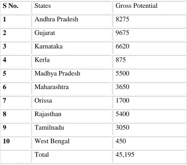
Table 1.1 GROSS POTENTIAL OF INDIA
S No.
States
Gross Potential
1
Andhra Pradesh
8275
2
Gujarat
9675
3
Karnataka
6620
4
Kerla
875
5
Madhya Pradesh
5500
6
Maharashtra
3650
7
Orissa
1700
8
Rajasthan
5400
9
Tamilnadu
3050
10
West Bengal
450
Total
45,195
5.2 CALCULATIONS
Total no of machines = 58 Total capacity = 13.5 MW Each machine capacity = 225/40 KW Minimum air velocity for the starting of wind turbine = 2m/s
Induction Generator
Over 1000 rpm Induction generator generate 40 KW Over 1500 rpm Induction generator generate 225 KW
Over 1650 rpm working must be stopped due to over speed fault
Height of windmill 30 m
Installation cost of per machine 1, 10, 00,000 Rs
Highest generation in a day 2, 02,900 KW
Date of highest generation 07/06/2003
Highest generation in a month 32,80,200kwh
Month of highest generation May 2002
Total Generation:
Production = 2686829 KWh Operating hours = 8429
Stopped hours = 12 Generator 1
Production = 22, 23,351 KWh Operating hours = 3,414
Mode = 1,234 times Speed = 1,500 rpm
Generator 2
Production = 4, 63,479 KWh Operating hours = 3,607
Mode = 6,089 times Speed = 1,000 rpm
Total hours in one year = 24 * 365 hours
= 8,760 hours
Operation time for generator 1(G1) = 3,414 hours Operation time for generator 2(G2) = 3,607 hours System fail time = 12 hours
Time when grid is not available = 76 hours in month Total hours in one year = 76 * 12 hours = 912 hours
Total Down time in a year = 912+12 = 924 hours Unavailability (FOR, q) = 924/ 924+8429 = 0.098 = 0.1 Availability (p) = 8429/ 924+8429 = 0.901 = 0.9
10.
CALCULATION FOR EXACT CAPACITY STATESWhen all units are available P(n) = ncr * pn-r * qr
Where
n = Total number of units r = number of units out p = availability
q = unavailability (FOR)
When all units are available then, n = 5 & r = 0
P(5) = 5c0 * 0.9(5-0) * 0.10 = 0.59049
When one unit is out then n = 5 & r = 1
P(4) = 5c1 * 0.9(5-1) * 0.11 = 0.32805
When two units is out then n = 5 & r = 2
P(3) = 5c2 * 0.9(5-2) * 0.12
= 0.0729
When three units is out then n = 5 & r = 3
P(2) = 5c3 * 0.9(5-3) * 0.13
= 0.0081 When Four units are out then
n = 5 & r = 4
P(1) = 5c4 * 0.9(5-4) * 0.14
= 0.00045 When all units are out then
n = 5 & r =5
P(0) = 5c5 * 0.9(5-5) * 0.15 = 0.00001
10.1.
CALCULATION FOR CUMULATIVE CAPACITY STATES:
A RECURSIVE ALGORITHM FOR CAPACITY MODEL BUILDING:The capacity model can be created using a simple algorithm which can also be used to remove a unit from the model. This approach can also be used for a multi-state unit, i.e. a unit which can exist in one or more Derated or partial output states as well as in the fully up and fully down states.
Case-1 NO DERATED STATES
The cumulative probability of a particular capacity outage state of X MW after a unit of capacity C MW and forced outage rate U is added is given by
P(X) = (1-U) P’(X) + (U) P’ (X-C) Eq. A
Where P’(X) and P(X) denote the cumulative probabilities of the capacity outage state of X MW before and after the unit is added. The above expression is initialized by setting P’(X) = 1.0 for X< 0 and P’(X) = 0 otherwise.
Case-2 DERATED STATES INCLUDED
Equation A can be modified as follows to include multi-state unit representations. n
P(X) = ∑ piP’(X - Ci) Eq. B i=1
where n= number of unit states
Ci=capacity outage of state I for the unit being added pi =probability of existence of the unit state i
when n=2, equation B reduces to equation A
now the system capacity outage probability is calculated sequentially as follows Total Up time = 8429 Hrs.
Total down time = 924 Hrs. A = 0.9
Hence U = 0.1
Step-1 Add the first unit:
P(0) = (1-0.1)1 + 0.1 P’(0-0) = 1
P(225) = (1-0.1)0 + 0.1P’ (225-225) = 0.1
Step-2 Add the second unit:
P(0) = (1-0.1)1 + 0.1*1 = 1
P(225) = (1-0.1)0.1 + 0.1 P’(225-225) = 0.19 P(450) = (1-0.1)0 + 0.1 P’(450-225) = 0.01 Step-3 Add the Third unit:
P(0) = (1-0.1)1 + 0.1(1) = 1
P(225) =(1-0.1)0.19 + 0.1 P’(225-225) = 0.271 P(450) = (1-0.1)0.01 + 0.1 P’(450-225) = 0.028 P(675) = (1-0.1)0 + 0.1 P’(675-225) = 0.001
Step-4 Add the Fourth unit:
P(0) = (1-0.1)1 + 0.1(1) = 1
P(225) = (1-0.1)0.271 + 0.1(1) = 0.3439 P(450) = (1-0.1)0.028 + 0.1(0.271) = 0.0523 P(675) = (1-0.1)0.001 + 0.1 (0.028) = 0.0037 P(900) = (1-0.1)0 + 0.1 (0.001) = 0.0001
Step-5 Add the Fifth unit:
P(0) = (1-0.1)1.0 + 0.1(1) = 1
P(225) = (1-0.1)0.3439 + 0.1(1) = 0.40951 P(450) = (1-0.1)0.0523 + 0.1(0.3439) = 0.08146 P(675) = (1-0.1)0.0037 + 0.1(0.0523) = 0.00856 P(900) = (1-0.1)0.0001 + 0.1(0.0037) = 0.000461 P(1125) = (1-0.1)0 + 0.1 (0.0001) = 0.00001
Step-6 Add the Sixth unit:
P(0) = (1-0.1)1 + 0.1(1) = 1
P(225) = (1-0.1)0.40951 + 0.1(1) = 0.468559
P(450) = (1-0.1)0.08146 + 0.1 (0.40951) = 0.114265 P(675) = (1-0.1)0.00856 + 0.1 (0.08146) = 0.01585 P(900) = (1-0.1)0.000461 + 0.1 (0.00856) = 0.0012709 P(1125) = (1-0.1)0.00001 + 0.1(0.000461) = 0.0000551 P(1350) = (1-0.1)0 + 0.1(0.00001) = 0.000001
Step-7 Add the Seventh unit:
P(0) =(1-0.1)1 + 0.1(1) = 1
P(225) = (1-0.1)0.468559 + 0.1(1) = 0.5217031
P(450) = (1-0.1)0.114265 + 0.1(0.468559) = 0.1496944 P(675) = (1-0.1)0.01585 + 0.1(0.114265) = 0.0256915 P(900) = (1-0.1)0.0012709 + 0.1(0.01585) = 0.00272881 P(1125) = (1-0.1)0.0000551 + 0.1(0.0012709) = 0.00017668 P(1350) = (1-0.1)0.000001 + 0.1(0.0000551) = 0.00000641 P(1575) = (1-0.1)0 + 0.1(0.000001) = 0.0000001
Step-8 Add the Eighth unit:
P(0) = (1-0.1)1 + 0.1(1) = 1
P(225) = (1-0.1)0.5217031 + 0.1(1) = 0.5695
P(450) = (1-0.1)0.1496944 + 0.1(0.5217031) = 0.1869 P(675) = (1-0.1)0.0256915 + 0.1(0.1496944) = 0.03809 P(900) = (1-0.1)0.00272881 + 0.00256915 = 0.00502 P(1125) = (1-0.1)0.00017668 + 0.000272881 = 0.000432 P(1350) = (1-0.1)0.00000641 + 0.000017668 = 0.0000234 P(1575) = (1-0.1)0.0000001 + 0.00000641 = 0.0000065 P(1800) = (1-0.1)0 + 0.1(0.0000001) = 0.00000001
Step-9 Add the Ninth unit:
P(0) = (1-0.1)1.0 + 0.1(1) = 1
P(225) = (1-0.1)0.5695 + 0.1(1) = 0.6126 P(450) = (1-0.1)0.1869 + 0.1(5695) = 0.2252 P(675) = (1-0.1)0.03809 + 0.1(0.1869) = 0.05297 P(900) = (1-0.1)0.00502 + 0.1(0.03809) = 0.00833 P(1125) = (1-0.1)0.000432 + 0.1(0.00502) = 0.00045 P(1350) = (1-0.1)0.0000234 + 0.1(0.000432) = 0.000064 P(1575) = (1-0.1)0.0000065 + 0.1(0.0000243) = 0.0000082 P(1800) = (1-0.1)0.00000001 + 0.1(0.0000065) = 0.00000066 P(2025) = (1-0.1)0 + 0.1(0.00000001) = 0.000000001
Step-10 Add the Tenth unit:
P(0) = (1-0.1)1.0 + 0.1(1) = 1
P(225) = (1-0.1)0.6126 + 0.1(1) = 0.65134 P(450) = (1-0.1)0.2252 + 0.1(0.6126) = 0.26394 P(675) = (1-0.1)0.05297 + 0.1(0.2252) = 0.070193 P(900) = (1-0.1)0.00833 + 0.1(0.05297) = 0.012794 P(1125) = (1-0.1)0.00045 + 0.1(0.00833) = 0.001238 P(1350) = (1-0.1)0.000064 + 0.1(0.00045) = 0.0001026 P(1575) = (1-0.1)0.0000082 + 0.1(0.000064) = 0.00001378 P(1800) = (1-0.1)0.00000066 + 0.1(0.0000082) = 0.000001414 P(2025) = (1-0.1)0.000000001 + 0.1(0.00000066) = 0.000000066 P(2250) = (1-0.1)0 + 0.1(0.000000001) = 0.0000000001
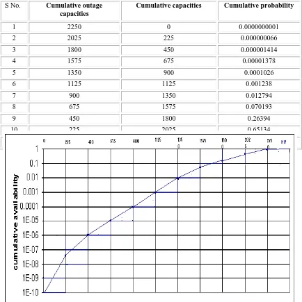
Table 2
RESULT OF DEWAS WIND POWER PLANT EXACT CAPACITY STATES No. Outage Capacities Available Capacities Probability
1 1125 000 0.00001
2 900 225 0.00045
3 675 450 0.0081
4 450 675 0.0729
5 225 900 0.32805
6 000 1125 0.59049
Table 3 RESULTS OF CUMULATIVE CAPACITY STATES
S No. Cumulative outage
capacities
Cumulative capacities Cumulative probability
1 2250 0 0.0000000001
2 2025 225 0.000000066
3 1800 450 0.000001414
4 1575 675 0.00001378
5 1350 900 0.0001026
6 1125 1125 0.001238
7 900 1350 0.012794
8 675 1575 0.070193
9 450 1800 0.26394
10 225 2025 0.65134
11 0 2250 1
Fig. 5.3.1 Cumulative capacity Vs cumulative availability
6.1 CONCLUSION
The case study of Dewas power plant Madhya Pradesh, India of 58 numbers of 225 KW each (13.5
MW).The reliability evaluation result of 10 units of Dewas plant connected to eastern grid were
estimated. The estimates are based on the performance data of the respective units over a period of one
year. As seen from the table in the beginning when all the units are in down state then the cumulative
probability of availability is very low 0.0000000001 and when the all 10 units are available the
cumulative probability of availability is 1. From each generating unit the probability of total generating
capacity not exceeding a given power level was computed using analytical method. The results were
shown in the form of graph. The graph is drawn between cumulative capacity state and cumulative
available probability. From the graph the system availability from the given capacity is evaluated. This
gives a measure of reliability of the system. The results presented give full insight into the generating
capacities of each unit. These can be taken as a guide to arrive at the deficit of energy that can be
expected. Thus the inevitable power cuts be planned in advance in rotational basis. The data also
pinpoints the weaker aspects of the generating system, which requires strengthen. The data can also be
used as a basis for reliability based expansion program of generating system, in order that future loads can
be served effectively. From above study it is also observed that the wind speeds from November to March
are low. This period is suitable for maintenance.
The power produced by the wind turbine increases from zero at the threshold wind speed (cut in speed)
(usually around 5m/s but varies with site) to the maximum at the rated wind speed. Above the rated wind
speed, (15 to 25 m/s) the wind turbine continues to produce the same rated power but at lower efficiency
until shut down is initiated if the wind speed becomes dangerously high, i.e. above 25 to 30m/s (gale
force). The exact specifications for energy capture by the turbine depend on the distribution of wind speed
over the year at the individual site. Air density has a significant effect on wind turbine performance. The
power available in the wind is directly proportional to air density. As air density increases the available
power also increases. Air density is a function of air pressure and temperature. It increases when air
pressure increases or the temperature decreases. Both temperature and pressure decrease with increasing
elevation. Consequently changes in elevation produce a profound effect on the generated power as a result
of changing in the air density.
REFERENCES
[1] R. Billinton, “Power System Reliability Evaluation”, Book, Gorodon & Breach, 1970, New York, USA.
[2] X. WANG & J.R.McDonald, ”Modern Power System Planning”,Book McGraw-HILL
[3] Shu Wang, “Reliability Assessment of Power Systems with Wind Power Generation” Thesis (A thesis submitted to the Graduate Faculty of North Carolina State University) 2008.
[4] R. Billinton, R. N. Allan, Reliability Evaluation of Engineering Systems: Concepts and Techniques, 2nd Edition, New York: Plenum Press, 1992.
[5] R. Billinton and R. N. Allan, “Reliability Evaluation of Power Systems”, 2nd Edition, New York: Plenum Press, 1996.
[6] M.D.Wadwa, “Wind data collection & Analyses of wind farms”, National conference on wind energy commercialization REC Bhopal, India , 1999 March, pp 171-177.
[7] Omar Badran, Emad Abdulhadi, Rustum Mamlook, “Evaluation of parameters affecting wind turbine generation”,
[8] Jun-Kyung Lee, In-Su Bae, Hyun-Soo Jung and Jin-O Kim, “Evaluating Reliability of Distributed Generation with Analytical Techniques”,
[9] J.F. Manwell, J. G. McGowan, and A. L. Rogers, “Wind Energy Explained:Theory, Design and Application”, New York: Wiley, 2002.
[10] J. Bhagwan Reddy, D.N. Reddy, “Reliability Evaluation of a Grid Connected Wind Farm – A case Study of Ramgiri Wind Farm in Andhra Pradesh, India”, IEEE 2004
[11] R. Piwko, G. Boukarim, K. Clark, G. Haringa, G. Jordan, N. Miller, Y. Zhou, and J. Zimberlin, “The effects of integrating wind power on transmission system planning, reliability, and operations phase 2,” GE Energy, Schenectady, NY, Feb. 2004.
[12] P. Flores, A. Tapia, and G. Tapia, “Application of a control algorithm for wind speed
Prediction and active power generation,” Renewable Energy, vol. 30, no. 4, pp 523-536, Apr. 2005.
[13] M. Ahlstrom, L. Jones, R. Zavadil, and W. Grant, “The future of wind forecasting and utility operations,” IEEE Power and energy Magazine, vol. 3, no. 6, pp. 57-64, Nov.-Dec. 2005.
[14] PJM Interconnection, [Online]. Available: http://www.pjm.com
[15] North American Electric Reliability Corporation [Online]. Available: http://www.nerc.com
[16] http://en.wikipedia.org/wiki/Wind_power
[17] http://en.wikipedia.org/wiki/Electricity_sector_in_India
[18] http://en.wikipedia.org/wiki/Wind_power_in_India
[19] M.P. Wind Farms Ltd. Dewas Wind Power Plant