Text dependent Forensic Voice Comparison: Likelihood Ratio Estimation with the Hidden Markov Model (HMM) and Gaussian Mixture Model

Text-dependent Forensic Voice Comparison: Likelihood Ratio

Estima-tion with the Hidden Markov Model (HMM) and Gaussian Mixture

Model – Universal Background Model (GMM-UBM) Approaches

Satoru Tsuge

Daido University, Japan [email protected]

Shunichi Ishihara

Australian National University [email protected]

Abstract

Among the more typical forensic voice comparison (FVC) approaches, the acous-tic-phonetic statistical approach is suitable for text-dependent FVC, but it does not fully exploit available time-varying infor-mation of speech in its modelling. The au-tomatic approach, on the other hand, es-sentially deals with text-independent cas-es, which means temporal information is not explicitly incorporated in the model-ling. Text-dependent likelihood ratio (LR)-based FVC studies, in particular those that adopt the automatic approach, are few. This preliminary LR-based FVC study compares two statistical models, the Hid-den Markov Model (HMM) and the Gaussian Mixture Model (GMM), for the calculation of forensic LRs using the same speech data. FVC experiments were car-ried out using different lengths of Japanese short words under a forensically realistic, but challenging condition: only two speech tokens for model training and LR estima-tion. Log-likelihood-ratio cost (Cllr) was

used as the assessment metric. The study demonstrates that the HMM system con-stantly outperforms the GMM system in terms of average Cllr values. However,

words longer than three mora are needed if the advantage of the HMM is to become evident. With a seven-mora word, for ex-ample, the HMM outperformed the GMM by a Cllr value of 0.073.

1 Introduction

After the DNA success story, the likelihood ratio (LR)-based approach became the new paradigm for evaluating and presenting forensic evidence in court. The LR approach has also been applied to speech evidence(Rose, 2006), and it is

increasing-ly accepted in forensic voice comparison (FVC) as well (Morrison, 2009).

There are two different approaches in FVC. They are the ‘acoustic-phonetic statistical ap-proach’ and the ‘automatic apap-proach’ (Morrison et al., 2018). The former usually works on compara-ble phonetic units that can be found in both the of-fender and suspect samples. In the latter, acoustic measurements are usually carried out over all por-tions of the available recordings, resulting in more detailed acoustic characteristics of the speakers. The common statistical models used in the auto-matic approach are the Gaussian mixture model – universal background model (GMM-UBM) (Reynolds et al., 2000) and i-vectors with proba-bilistic linear discrimination analysis (PLDA) (Burget et al., 2011). Due to its nature, the auto-matic approach is mainly used for text-‘independent’ FVC, and there is a good amount of research on this (Enzinger & Morrison, 2017; Enzinger et al., 2016). The acoustic-phonetic sta-tistical approach is a type of text-‘dependent’ FVC because it tends to focus on particular linguistic units, such as phonemes, words, phrases, etc. Hav-ing said that, even if one is targetHav-ing a particular word or phrase, for example ‘hello’, all obtainable features are not exploited in the acoustic-phonetic statistical approach because it still tends to focus on particular segments or phonemes of the word or phrase, e.g. the formant trajectories of the diph-thong and the static spectral information of the fricative (Rose, 2017).

One of the advantages of text-dependent FVC is the availability of the time-varying characteris-tics of a speaker, which is information that can be explicitly included in the modelling.

There are a good number of LR-based text-independent FVC studies in the automatic ap-proach (Enzinger & Morrison, 2017; Enzinger et al., 2016). However, although there are some

ies in which text-independent models (e.g. GMM) were applied to text-dependent FVC scenarios (Morrison, 2011), to the best of our knowledge, studies on LR-based text-dependent FVC in the automatic approach are scarce.

In this study, a text-dependent LR-based FVC system with the GMM-UBM based system (GMM system) and that with the hidden Markov model (HMM system) are compared in their per-formance using the same data. The transitional characteristic of individual speech can be explicit-ly modelled in the latter system.

Words of various length are used for testing purposes to see how word duration influences the performance of the systems. Having the forensi-cally realistic condition of data sparsity in mind, we used only two tokens of each word for model-ling and testing.

It is naturally expected that, given a sufficient amount of data, the HMM system outperforms the GMM system. However, it is not so clear whether the above expectation is realistic when the amount of data is limited. Even if the HMM system works better, it is important to establish how the HMM and GMM systems compare with respect to the calculation of strength of LR, and also how and under what conditions the former is more advan-tageous than the latter.

2 Likelihood Ratios

The LR framework has been advocated by many as the logically and legally correct framework for assessing forensic evidence and reporting the out-come in court (Aitken, 1995; Aitken & Stoney, 1991; Aitken & Taroni, 2004; Balding & Steele, 2015; Evett, 1998; Robertson & Vignaux, 1995). A substantial amount of fundamental research on FVC has been carried out since the late 1990s (Gonzalez-Rodriguez et al., 2007; Morrison, 2009; Rose, 2006), and it is now accepted in an increasing number of countries (Morrison et al., 2016).

In the LR framework, the task of the forensic expert is to estimate strength of evidence and re-port it to the court. LR is a measure of the quanti-tative strength of evidence, and is calculated using the formula in 1).

In 1), E is the evidence, i.e. the measured

prop-erties of the voice evidence; p(E|Hp) is the

proba-bility of E, given Hp, in other words the

prosecu-tion or same-speaker hypothesis; p(E|Hd) is the

probability of E, given Hd, in other words the

de-fence or different-speaker hypothesis (Robertson & Vignaux, 1995). The LR can be considered in terms of the ratio between similarity and typicali-ty. Similarity here means the similarity of evi-dence attributable to the offender and the suspect, respectively. Typicality means the typicality of that evidence against the relevant population.

The relative strength of the given evidence with

respect to the competing hypotheses (Hp vs. Hd) is

reflected in the magnitude of the LR. If the evi-dence is more likely to occur under the prosecu-tion hypothesis than under the defence hypothesis, the LR will be higher than 1. If the evidence is more likely to occur under the defence hypothesis than under the persecution hypothesis, the LR will be lower than 1. For example, LR = 30 means that the evidence is 30 times more likely to occur on the assumption that the evidence is from the same person than on the assumption that it is not.

The important point is that the LR is concerned with the probability of the evidence, given the

hy-pothesis (either Hp or Hd). The probability of the

evidence can be estimated by forensic scientists. They legally must not and logically cannot esti-mate the probability of the hypothesis, given the evidence. This is because the forensic scientist is not legally in a position to refer to the ultimate ‘guilty vs. non-guilty’ question, i.e. the probability of the hypothesis, given the evidence. That is the task of the trier-of-fact. Furthermore, the forensic scientist would need to refer to the Bayesian theo-rem to estimate the probability of the hypothesis, given the evidence, using prior information that is only accessible to the trier-of-fact; thus the foren-sic scientist cannot logically estimate the probabil-ity of the hypothesis.

3 Experimental Design

In this section, the nature of the database used for the experiments is explained first. This is followed by an illustration as to how the speaker compari-sons were set up for the experiments. The acoustic features used in this study will be explained

to-wards the end.

3.1 Database

Our data were extracted from the National Re-search Institute of Police Science (NRIPS)

data-LR=p(E|Hp)

base (Makinae et al., 2007). The database consists of recordings collected from 316 male and 323 female speakers. All utterances were read-out speech, consisting of single syllables, words, se-lected sentences and so on. The word-based re-cordings stored in the database provided the data used in this study.

Participants ranged in age from 18 to 76 years. The metadata provide information on the areas of Japan (or overseas in some cases) where they have resided, as well as their height, weight, and their health conditions on the day of recording. Only male speakers who completed the recordings in two different sessions separated by 2-3 months, without any mis-recordings for the target 66 words, were selected for the current study (result-ing in 310 speakers). Each word was recorded on-ly twice in each session.

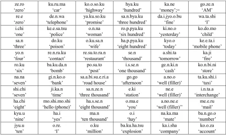
The rhythmic unit of Japanese is the mora. Based on mora, the 66 words, all listed in Table 1, consist of 25 two-, 16 three-, 22 four-, 2 five- and 1 seven-mora words.

The 310 speakers were separated into six dif-ferent, mutually exclusive groups: Gr1 (59 speak-ers), Gr2 (60), Gr3 (60), Gr4 (60), Gr5 (60) and Gr6 (13). Five different experiments were con-ducted using the six groups, as shown in Table 2.

The test database was used for simulating two types of offender-suspect comparisons: same-speaker (SS) and different-same-speaker (DS). An LR

was estimated for each of the comparisons. The development database was also called upon for simulating offender-suspect comparisons, but the derived scores (pre-calibration LRs) were specifi-cally used to obtain the weights for calibration (re-fer to §4.4 for details on calibration). The back-ground database was used to build the statistical model for typicality.

As mentioned earlier, there are two recordings per speaker for each word in each session. The suspect model was built using two recordings tak-en from one session, and an LR was estimated for each of the two recordings of the other session (offender evidence). The same process was re-peated by swapping the recordings of the sessions. In this way, 4 LRs were obtained for each SS comparison, and 8 LRs for each DS comparison.

Thus, the number of comparisons is 4*n (n =

number of speakers) for the SS comparisons, and

8*nC2 (C=combination) for the DS comparisons.

Using the five different groups (Gr1~5) separately

ze.ro ‘zero’ ku.ru.ma ‘car’ ko.o.so.ku ‘highway’ hya.ku ‘hundred’ ka.ne ‘money’;= go.ze.n ‘AM’ re.e ‘zero’ de.n.wa ‘telephone’ ya.ku.so.ku ‘promise’ sa.n.bya.ku ‘three hundred’ da.i.jyo.o.bu ‘fine’ wa.ta.shi ‘I’ i.chi ‘one’ ke.e.sa.tsu ‘police’ o.n.na ‘woman’ ro.p.pya.ku ‘six hundred’ ki.no.o ‘yesterday’ ko.do.mo ‘child’ sa.n ‘three’ do.ku ‘poison’ o.ku.sa.n ‘wife’ ha.p.pya.ku ‘eight hundred’ kyo.o ‘today’ ke.e.ta.i ‘mobile phone’ yo.n ‘four’ re.n.ra.ku ‘contact’ re.su.to.ra.n ‘restaurant’ se.n ‘thousand’ a.shi.ta ‘tomorrow’ ka.ji ‘fire’ ro.ku ‘six’ ba.ku.da.n ‘bomb’ po.su.to ‘post’ i.s.se.n ‘one thousand’ ge.n.ki.n ‘cash’ ko.n.bi.ni ‘store’ na.na ‘seven’ gi.n.ko.o ‘bank’ sa.a.bi.su.e.ri.a ‘road house’ go.go ‘afternoon’ a.no.o ‘well (filler)’ ta.ku.shi.i ‘taxi’ shi.chi ‘seven’ ji.ka.n ‘time’ sa.n.ze.n ‘three thousand’ e.ki ‘station’ ne.e ‘well (filler)’ i.n.ta.a ‘interchange’ ha.chi ‘eight’ mo.shi.mo.shi ‘hello (phone)’ ha.s.se.n ‘eight thousand’ o.ma.e ‘you’ a.no.ne.e ‘well (filler)’’ me.e.ru ‘mail’ kyu.u ‘nine’ ha.i ‘yes’ ma.n ‘ten thousand’ o.i ‘hay’ na.ka.ma ‘mate’ ba.n.go.o ‘number’ jyu.u ‘ten’ o.re. ‘I’ o.ku ‘million’ ba.ku.ha.tsu ‘explosion’ ka.i.sha ‘company’ ko.o.za ‘account’ Table 1: 66 target words with their glosses. Each mora is separated by a period.

Experiments Test Dev Back

Exp1 Gr1 Gr2 Gr3,4,5,6

Exp2 Gr2 Gr3 Gr1,4,5,6

Exp3 Gr3 Gr4 Gr1,2,5,6

Exp4 Gr4 Gr5 Gr1,2,3,6

Exp5 Gr5 Gr1 Gr2,3,4,6

Table 2: Usage of Gr1~6 for experiments (Exp). Test, Dev and Back refer to test, development and

as a test database, it was possible, altogether, to carry out 1188 SS comparisons and 69392 DS comparisons. The breakdowns of the SS and DS comparisons are given in Table 3 for the five ex-periments (Exp1~5).

The NRIPS database also contains the record-ings of 50 sentences that are based on ATR pho-netically balanced Japanese sentences (Kurematsu et al., 1990). These sentences were used to build the initial statistical models (refer to §4.1 and §4.2 for details).

3.2 Acoustic Features

Twelve mel-frequency cepstral coefficients (MFCCs), 12 Δ MFCCs and Δ log power (a

fea-ture vector of 25th_{-order) were extracted with a 20}

msec wide hamming window shirting every 10 msec.

4 Estimation of Likelihood Ratios

In this section, the two different modelling tech-niques used in the current study are explained. This is followed by an exposition of the method for calculating scores with these models. The method used for converting the scores to the LRs, namely calibration, will be explained last.

For this study, the suspect model, rather than being based solely on the data of the suspect speaker, was generated by adapting a speaker-unspecific model (background model) by means of a maximum a posteriori (MAP) procedure. Three different numbers of Gaussians (4, 8 and 16) were tried in the models.

4.1 GMM Models

The following is the process of building a er-specific word-dependent GMM for each speak-er.

1) To build a speaker-unspecific

word-independent GMM using the recordings of the phonetically balanced utterances;

2) To build a speaker-unspecific word-dependent

GMM for each word by training the

speaker-unspecific word-independent GMM, which was generated in 1), with the relevant word recordings of the background database;

3) To build the speaker-specific word-dependent

GMM (suspect model = λsus) for each word by

training the speaker-unspecific

word-independent GMM, which was built in 2), with the speaker specific data in the test data-base, while applying a MAP adaptation.

The speaker-unspecific word-dependent GMM, which was built in 2) for each word, was used as the background model (λbkg).

4.2 HMM Models

The following is the process of building a er-specific word-dependent HMM for each speak-er.

1) To build speaker-unspecific

phoneme-dependent HMMs using the recordings of the phonetically balanced utterances;

2) To build an initial speaker-unspecific

word-dependent HMM for each word by

concate-nating speaker-unspecific

phoneme-dependent HMMs, which were built in 1).

3) To build speaker-specific word-dependent

HMM (suspect model = λsus) by training the initial speaker-unspecific word-dependent HMM, which was built in 2), with the speaker specific data in the test database, while apply-ing a MAP adaptation.

The initial speaker-unspecific word-dependent HMM, which was built in 2), was trained with the relevant word recordings of the background data-base, and the resultant model was used as the speaker-unspecific word-dependent background model (λbkg).

4.3 Score Calculations

The score of each comparison can be estimated using the equation given in 2), in which s = score,

xt = an observation sequence of vectors of

acous-tic features constituting the offender data of which

there are a total of T, λsus = suspect model and λbkg

= background model.

𝑠 = 1

𝑇∑ log(𝑝(𝑥𝑡|𝜆𝑠𝑢𝑠))

𝑇

𝑡=1

− log (𝑝(𝑥𝑡|𝜆𝑏𝑘𝑔))

2)

Experiments SS DS

Exp1: Gr1 (59) 236 13688

Exp2: Gr2 (60) 240 14160

Exp3: Gr3 (60) 240 14160

Exp4: Gr4 (58) 232 13224

Exp5: Gr5 (60) 240 14160

Total 1188 69392

A score is estimated as the mean of the relative values of the two probability density functions for the feature vectors extracted from the offender da-ta, and was calculated for each of the SS and DS comparisons.

4.4 Scores to Likelihood Ratios

The outcomes of the GMM and HMM systems

are not LRs, but are known as scores. The value of

a score provides information about the degree of the similarity between the two speech samples, i.e. the offender and suspect samples, having taken in-to account their typicality with respect in-to the rele-vant population; it is not directly interpretable as an LR (Morrison, 2013, p. 2). Thus, the scores need to be converted to LRs by means of a cali-bration process. As we will see in §6, calicali-bration is an essential part of LR-based FVC.

Logistic-regression calibration (Brümmer & du Preez, 2006) is a commonly used method that converts scores to interpretable LRs by applying linear shifting and scaling in the log odds space. A

logistic-regression line (e.g. y = ax + b; x = score;

y = log10LR) whose weights (i.e. a and b in y = ax

+ b) are estimated from the SS and DS scores of

the development database is used to

monotonical-ly shift (by the amount of b) and scale (by the

amount of a) the scores of the testing database to

the log10LRs.

5 Assessment Metrics

A common way of assessing the performance of a classification system is with reference to its correct- or incorrect-classification rate: for in-stance, how many of the SS comparisons were correctly assessed as coming from the same speakers, and how many of the DS comparisons were correctly assessed as coming from different speakers. In the context of LR-based FVC, an LR can be used as a classification function with LR = 1 as unity. However, correct- or incorrect-classification rate is a binary decision (same speaker or different speakers), which refers to the ultimate issue of ‘guilty vs. non-guilty’. As plained in §2, it is not the task of the forensic ex-pert, but of the trier-of-fact, to make such a deci-sion. Thus, any metrics based on binary decision are not coherent with the LR framework.

As emphasised in §2, the task of the forensic expert is to estimate the strength of evidence as accurately as possible, and the strength of evi-dence, which can be quantified by means of a LR,

is not binary in nature, but continuous. For exam-ple, both LR = 10 and LR = 20 support the correct hypothesis for the SS comparisons, but the latter supports the hypothesis more strongly than the former. The relative strength of the LR needs to be taken into account in the assessment.

Hence, in this study, the log-likelihood-ratio

cost (Cllr), which is a gradient metric based on

LR, was used as the metric for assessing the per-formance of the LR-based FVC system. The

cal-culation of Cllr is given in 3) (Brümmer & du

Preez, 2006).

Cllr=1 2

( 1

NH_p∑ log2(1+

1 LRi) N_Hp

i forHp=true

+

1 NHd

∑ log2(1+LRj)

N_Hd

j forH_d=true ₎

3)

In 3), NHp and NHd are the number of SS and

DS comparisons, and LRi and LRj are the linear

LRs derived from the SS and DS comparisons, re-spectively. Under a perfect system, all SS compar-isons should produce LRs greater than 1, since or-igins are identical; as, in the case of DS compari-sons, origins are different, DS comparisons should

produce LRs less than 1. Cllr takes into account

the magnitude of derived LR values, and assigns

them appropriate penalties. In Cllr, LRs that

sup-port the counter-factual hypotheses or, in other words, contrary-to-fact LRs (LR < 1 for SS com-parisons and LR > 1 for DS comcom-parisons) are heavily penalised and the magnitude of the penal-ty is proportional to how much the LRs deviate from unity. Optimum performance is achieved

when Cllr = 0 and decreases as Cllr approaches and

exceeds 1. Thus, the lower the Cllr value, the better

the performance.

The Cllr measures the overall performance of a

system in terms of validity based on a cost func-tion in which there are two main components of

loss: discrimination loss (Cllrmin) and calibration

loss (Cllrcal) (Brümmer & du Preez, 2006). The

former is obtained after the application of the so-called pooled-adjacent-violators (PAV) transfor-mation – an optimal non-parametric calibration procedure. The latter is obtained by subtracting

the former from the Cllr. In this study, besides Cllr,

Cllrmin and Cllrcal are also referred to.

6 Experimental Results and Discussions

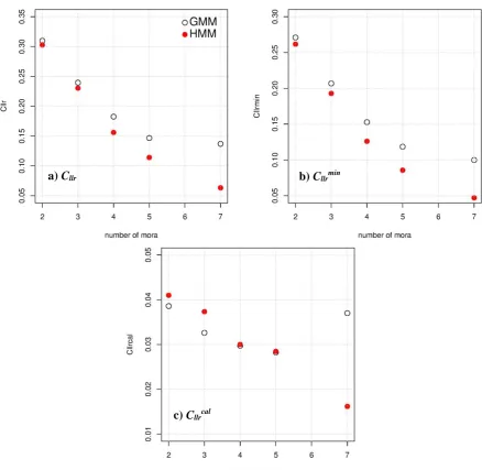
The average Cllr, Cllrmin and Cllrcal values were

cal-culated according to the mora numbers; they are plotted in Figure 1 as a function of word duration, separately for the HMM and GMM systems. The numerical values of Figure 1 are given in Table 4.

Although this was expected, it can be seen from Figure 1a and Table 4 that the overall

perfor-mance (Cllr) of both systems improves as the

words become longer in terms of mora, and also that the HMM system constantly outperforms the

GMM system as far as average Cllr values are

concerned. The performance gap between the two systems becomes wider as the number of mora in-creases, with the performance of the two systems being similar with words of two and three moras. For 12 out of the 25 two-mora words and 6 out of the 16 three-mora words, the GMM system per-formed better than the HMM system in terms of

Cllr. In other words, the evidence suggests that the

HMM may not be clearly advantageous for short words, e.g. two- or three-mora words. For the sake of reference, for only 6 out of the 22 four-mora words, the GMM system outperformed the HMM system. For the five- and seven-mora words, the HMM system constantly outperformed the GMM system.

The discriminability of the systems (Cllrmin)

(Figure 1b) also exhibits the same trend as the overall performance in that discriminability im-proves with more moras, the HMM system con-stantly performed better than the GMM system, and the performance of the former improves at a faster rate than that of the latter. As a result, there is a larger gap in discriminability between the two systems with the seven-mora word (0.052 = 0.099-0.047) than there is with the two-mora words (0.009 = 0.270-0.261).

The calibration loss of both systems (Cllrcal)

(Figure 1c) is very similar for two-, three-, four- and five-mora words, which are essentially the same for the two systems (2: 0.038 and 0.040; 3: 0.032 and 0.037; 4: 0.029 and 0.030; 5: 0.028 and

0.028). The calibration loss improves (albeit at a very small rate) as a function of word duration, except in the case of the GMM system with the seven-mora word.

As has been described by means of Figure 1 and Table 4, it is clearly advantageous to include temporal information in modelling in Japanese, even under the challenging condition of data spar-sity. However, the difference in performance may not be evident with short, e.g. two- and three-mora, words. Put differently, if a forensic speech expert is working on a comparable word or phrase of relatively good length, the decision to either in-clude transitional information in the modelling or not is likely to substantially impact on the out-come. For example, the HMM system

outper-formed the GMM system by the Cllr values of

0.073 (= 0.136 - 0.063) with the seven-mora word.

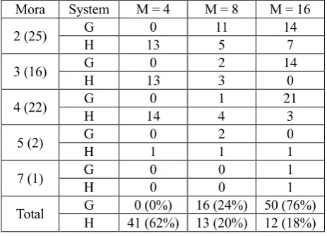
Three different numbers of Gaussians – 4, 8 and 16 – were used in the study. Table 5 shows which mixture number of Gaussians performed best for words of different mora duration accord-ing to the different systems. For example, out of the 25 two-mora words, the GMM system with a mixture number of 8 (M = 8) returned the best re-sult for 11 words, and the HMM system with a mixture number of 4 (M = 4) yielded the lowest

Cllr value for 13 words.

According to Table 5, there is a clear difference between the two systems with respect to the best performing mixture number of Gaussians, in that the GMM tends to require a higher mixture num-ber for optimal performance (overall, 76% of words worked best with a mixture number of 16), while the HMM generally does not require a

2 3 4 5 7

Cllr G 0.309 0.239 0.182 0.146 0.136

H 0.302 0.230 0.156 0.114 0.063 Cllrmin G 0.270 0.206 0.152 0.118 0.099

H 0.261 0.192 0.126 0.085 0.047 Cllrcal G 0.038 0.032 0.029 0.028 0.037

H 0.040 0.037 0.030 0.028 0.016 Table 4: Numerical information of Figure 1.

G = GMM and H = HMM.

Mora System M = 4 M = 8 M = 16

2 (25) G _{H 13} 0 11 ₅ 14 ₇

3 (16) G _H 0 2 14

13 3 0

4 (22) G 0 1 21

H 14 4 3

5 (2) G 0 2 0

H 1 1 1

7 (1) G 0 0 1

H 0 0 1

Total G 0 (0%) 16 (24%) 50 (76%) H 41 (62%) 13 (20%) 12 (18%) Table 5: Best-performing Gaussian numbers (M) for

higher mixture number (overall, 62% of words performed best with a mixture number of 4).

To investigate whether there are any differences in the nature and magnitude of the derived LRs, a Tippett plot was generated for each word in each experiment, and this was done separately for the GMM and HMM systems. Figure 2 has Tippett plots of the five-mora word ‘daijyoobu’ with 16 Gaussians: Panel a) = GMM and Panel b) = HMM. The plots are fairly typical and illustrate

the differences between the two systems.

Tippet plots show the cumulative proportion of the LRs of the DS comparisons (DSLRs), which are plotted rising from the right, as well as of the LRs of the SS comparisons (SSLRs), plotted ris-ing from the left. The solid curves are for LRs and

the dotted curves are for scores (pre-calibration LRs). For all Tippett plots, the cumulative propor-tion of trails is plotted on the y-axis against the log10 LRs on the x-axis.

As can be seen in Figure 2, the derived scores (pre-calibration LRs), which are given in dotted curves, are uncalibrated in different ways for the GMM and HMM systems: the former (Figure 2a) is uncalibrated to the left and the latter (Figure 2b) is uncalibrated to the right. This indicates that cal-ibration is essential in both systems. In fact, cali-brating system output is recommended as standard practice (Morrison, 2018).

The dotted curves are more widely apart in Figure 2a (GMM) than in Figure 2b (HMM). This means that the magnitude of the derived scores is

Figure 1: Cllr (Panel a), Cllrmin (b) and Cllrcal (c) values are plotted as a function of mora duration, separately for

GMM (empty circle) and HMM (filled circle) systems. Note that the Y-axis scale in Panel c is different from that in Panels a and b.

a) Cllr b) Cllrmin

greater with the GMM system than with the HMM system. However, after calibration (solid curves), it can be seen that the magnitude of the DSLRs is very similar between the two systems while the SSLRs are far stronger for the HMM system than for the GMM system. That is, the cal-ibration causes different effects in the two sys-tems; it brings about more conservative LRs for the GMM system, but enhanced LRs for the HMM system.

Although calibration usually results in a better performance, its impact on the magnitude of LRs seems to be different depending on various fac-tors, including the types of features and modelling techniques. Many FVC studies, in particular those based on the acoustic-phonetic statistical ap-proach, report that calibration results in more

con-servative LRs than scores (Rose, 2013), while it contributes to stronger LRs for the automatic ap-proach (Morrison, 2018). However, it is not clear at this stage what the observed differences be-tween the two systems with respect to the rela-tionship between the scores and LRs entail. This warrants further investigation.

Apart from the similar degree of magnitude of the DSLRs (including both consistent-with-fact and contrary-to-fact LRs) that were obtained for the GMM and HMM systems, Figure 2 shows that the magnitude of the consistent-with-fact SSLRs is far greater for the HMM system (Figure 2b), and also that all of the SS comparisons were accurately classified as being from the same speakers for the HMM system. As a result, the

HMM system is assessed to be better in Cllr than

the GMM system (GMM: Cllr = 0.182 and HMM:

Cllr = 0.156).

7 Conclusions

This is a preliminary study investigating the use-fulness of speaker-individuating information man-ifested in the time-varying aspect of speech in a text-dependent FVC system, in particular in the automatic FVC approach. In this study, perfor-mance of the GMM and HMM systems was com-pared using the same data under a forensically re-alistic, but challenging condition, which is sparsi-ty of data. Even with short durations of two-, three-, four-, five- and seven-mora words, the HMM system constantly outperformed the GMM

system in terms of average Cllr values. However,

the benefits of the transitional information become evident when the HMM system is built with words longer than two- or three mora. With a sev-en-mora word, for example, the HMM system

performed better than the GMM system by a Cllr

value of 0.073.

This study also demonstrates that the outcomes (scores) of the GMM and HMM systems are not well-calibrated; thus calibration is an essential part of the FVC if they are to be used as models in the system.

Acknowledgments

The authors thank the reviewers for their valuable comments.

Figure 2: Tippett plots of the five-mora word ‘daijyoobu’ (Exp5) with 16 Gaussians: Panel a) =

GMM and Panel b) = HMM a) GMM

References

Aitken, C. G. G. (1995). Statistics and the Evaluation of Evidence for Forensic Scientists. Chichester: John Wiley.

Aitken, C. G. G., & Stoney, D. A. (1991). The Use of Statistics in Forensic Science. New York; London: Ellis Horwood.

Aitken, C. G. G., & Taroni, F. (2004). Statistics and the Evaluation of Evidence for Forensic Scientists. Chichester: John Wiley & Sons.

Balding, D. J., & Steele, C. D. (2015). Weight-of-evidence for Forensic DNA Profiles. Chichester: John Wiley & Sons.

Brümmer, N., & du Preez, J. (2006). Application-independent evaluation of speaker detection. Computer Speech and Language, 20(2-3), 230-275. Burget, L., Plchot, O., Cumani, S., Glembek, O.,

Matějka, P., & Brümmer, N. (2011). Discriminatively trained probabilistic linear discriminant analysis for speaker verification. Proceedings of the Acoustics, Speech and Signal Processing (ICASSP), 2011 IEEE International Conference on, 4832-4835.

Enzinger, E., & Morrison, G. S. (2017). Empirical test of the performance of an acoustic-phonetic approach to forensic voice comparison under conditions similar to those of a real case. Forensic Science International, 277, 30-40.

Enzinger, E., Morrison, G. S., & Ochoa, F. (2016). A demonstration of the application of the new paradigm for the evaluation of forensic evidence under conditions reflecting those of a real forensic-voice-comparison case. Science & Justice, 56(1), 42-57.

Evett, I. W. (1998). Towards a uniform framework for reporting opinions in forensic science casework. Science & Justice, 38(3), 198-202.

Gonzalez-Rodriguez, J., Rose, P., Ramos-Castro, D., Toledano, D. T., & Ortega-Garcia, J. (2007). Emulating DNA: Rigorous quantification of evidential weight in transparent and testable forensic speaker recognition. Ieee Transactions on Audio Speech and Language Processing, 15(7), 2104-2115.

Kurematsu, A., Takeda, K., Sagisaka, Y., Katagiri, S., Kuwabara, H., & Shikano, K. (1990). Atr Japanese Speech Database as a Tool of Speech Recognition and Synthesis. Speech Communication, 9(4), 357-363.

Makinae, H., Osanai, T., Kamada, T., & Tanimoto, M. (2007). Construction and preliminary analysis of a large-scale bone-conducted speech database. Proceedings of the Institute of Electronics,

information and Communication Engineers, 97-102.

Morrison, G. S. (2009). Forensic voice comparison and the paradigm shift. Science & Justice, 49(4), 298-308.

Morrison, G. S. (2011). A comparison of procedures for the calculation of forensic likelihood ratios from acoustic-phonetic data: Multivariate kernel density (MVKD) versus Gaussian mixture model-universal background model (GMM-UBM). Speech Communication, 53(2), 242-256.

Morrison, G. S. (2013). Tutorial on logistic-regression calibration and fusion: Converting a score to a likelihood ratio. Australian Journal of Forensic Sciences, 45(2), 173-197.

Morrison, G. S. (2018). The impact in forensic voice comparison of lack of calibration and of mismatched conditions between the known-speaker recording and the relevant-population sample recordings. Forensic Science International, 283, E1-E7.

Morrison, G. S., Enzinger, E., & Zhang, C. (2018). Forensic Speech Science. In I. Freckelton & H. Selby (Eds.), Expert Evidence. Sydney, Australia: Thomson Reuters.

Morrison, G. S., Sahito, F. H., Jardine, G., Djokic, D., Clavet, S., Berghs, S., & Dorny, C. G. (2016). INTERPOL survey of the use of speaker identification by law enforcement agencies. Forensic Science International, 263, 92-100. Reynolds, D. A., Quatieri, T. F., & Dunn, R. B.

(2000). Speaker verification using adapted Gaussian mixture models. Digital Signal Processing, 10(1-3), 19-41.

Robertson, B., & Vignaux, G. A. (1995). Interpreting Evidence: Evaluating Forensic Science in the Courtroom. Chichester: John Wiley.

Rose, P. (2006). Technical forensic speaker recognition: Evaluation, types and testing of evidence. Computer Speech and Language, 20 (2-3), 159-191.

Rose, P. (2013). More is better: Likelihood ratio-based forensic voice comparison with vocalic segmental cepstra frontends. International Journal of Speech, Language and the Law, 20(1), 77-116. Rose, P. (2017). Likelihood ratio-based forensic voice