University of South Carolina
Scholar Commons
Theses and Dissertations
1-1-2013
Spectral Analysis of Randomly Generated
Networks With Prescribed Degree Sequences
Clifford Davis Gaddy
University of South CarolinaFollow this and additional works at:https://scholarcommons.sc.edu/etd Part of theMathematics Commons
This Open Access Thesis is brought to you by Scholar Commons. It has been accepted for inclusion in Theses and Dissertations by an authorized administrator of Scholar Commons. For more information, please [email protected].
Recommended Citation
Spectral Analysis of Randomly Generated Networks with
Prescribed Degree Sequences
by
Clifford Davis Gaddy
Bachelor of Arts
Washington and Lee University 2010
Submitted in Partial Fulfillment of the Requirements
for the Degree of Master of Arts in
Mathematics
College of Arts and Sciences
University of South Carolina
2013
Accepted by:
Éva Czabarka, Major Professor
Linyuan Lu, Second Reader
c
Acknowledgments
First of all, I want to say thank you to my advisor Dr. Éva Czabarka. From my
first semester here, she has been extremely helpful and eager to discuss any topic
I was curious about. She has given me much personal, career, and mathematical
advice during the last two years. Thank you for leading me through this thesis and
the enormous amount of time that you have invested. You have made this whole
process and my time at the University of South Carolina a very enjoyable experience.
Thank you to Dr. Linyuan Lu for being the second reader of my thesis. I enjoyed
taking Probabilistic Methods with you in the fall. It was an extremely interesting
course and during this whole year, you have been very willing to discuss anything
with me. I thank you for that. Thank you to Dr. Zoltán Toroczkai for introducing
me to this project and giving me the network data that was fundamental to this
project. Thanks to Dr. Aaron Duttle for the discussions that we have had this year
regarding graphs and Markov chains. Also thanks for introducing me to the program
Geogebra that allows one to draw graphs. Thanks to Dr. László Székely for helpful
discussions throughout the thesis process, especially with regards to enumeration of
graphs with a given degree sequence and Markov chains. I also enjoyed your Discrete
mathematics class this year. Thank you to Dr. Richard Anstee, an extremely friendly
person full of advice. Thanks to Dr. George Mcnulty and Dr. Francisco Blanca-Silva
for help with Latex. Thanks to the technical staff of the mathematics department
for giving me extra hard drive space to store all my data. Lastly, thanks to all of
my friends and family for the loving support during the last two years: my Mom
Toby, Pat and Steph; and my two best friends Jordan and Asel, who have supported
me all along. And lastly, thanks to the other graduate students for long hours spent
Abstract
Network science attempts to capture real-world phenomenon through mathematical
models. The underlying model of a network relies on a mathematical structure called
a graph. Having seen its early beginnings in the 1950’s, the field has seen a surge of
interest over the last two decades, attracting interest from a range of scientists
in-cluding computer scientists, sociologists, biologists, physicists, and mathematicians.
The field requires a delicate interplay between real-world modeling and theory, as
it must develop accurate probabilistic models and then study these models from a
mathematical perspective. In my thesis, we undertake a project involving computer
programming in which we generate random network samples with fixed degree
se-quences and then record properties of these samples. We begin with a real-world
network, from which we extract a sample of at least one-hundred vertices through
the use of snowball sampling. We record the degree sequence, D, of this sample and
then generate random models with this same degree sequence. To generate these
models, we use a well-known graph algorithm, the Havel-Hakimi algorithm, to
pro-duce an initial non-random sample GD. We then run a Monte Carlo Markov Chain
(MCMC) on the sample space of graphs with this degree sequence beginning at GD
in order to produce a random graph in this space. Denote this random graph by
HD. Lastly, we compute the eigenvalues of the Laplacian matrix of HD, as these
eigenvalues are intricately connected with the structure of the graph. In doing this,
we intend to capture local properties of the network captured by the degree sequence
Table of Contents
Acknowledgments . . . iii
Abstract . . . v
List of Tables . . . vii
List of Figures . . . viii
Chapter 1 Background . . . 1
1.1 Introduction . . . 1
1.2 Graph Theory . . . 3
1.3 Probability . . . 7
1.4 History . . . 11
Chapter 2 Project . . . 18
2.1 Degree Sequence . . . 18
2.2 Markov Chains . . . 28
2.3 Laplacian Spectrum . . . 32
2.4 Program . . . 36
2.5 Results . . . 41
Bibliography . . . 44
Appendix A Code. . . 47
List of Tables
List of Figures
Figure 1.1 Representation of real life problem as a network . . . 3
Figure 1.2 Example Graph . . . 6
Figure 2.1 Switch in which {v1, v4} and {v3, v5} are deleted, and {v1, v5}
and {v3, v4} are added . . . 19
Figure 2.2 Iterations of Havel-Hakimi algorithm for degree sequence (3,3,3,2,1) 23
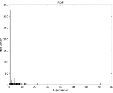
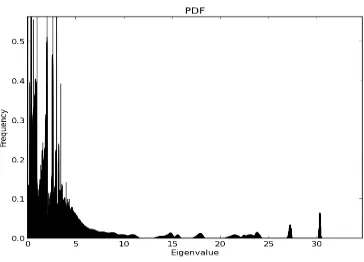
Figure B.1 Spectrum of Network Sample 1 . . . 60
Figure B.2 Degree Multiplicity of Degree Sequence of Network Sample 1 . . . 61
Figure B.3 Spectrum of MCMC Generated Graphs with Degree Sequence
of Network Sample 1 . . . 62
Figure B.4 Zoomed in view of Figure B.3 . . . 62
Figure B.5 Spectrum of Network Sample 2 . . . 63
Figure B.6 Degree Multiplicity of Degree Sequence of Network Sample 2 . . . 63
Figure B.7 Spectrum of MCMC Generated Graphs with Degree Sequence
of Network Sample 2 . . . 64
Figure B.8 Zoomed in view of Figure B.7 . . . 64
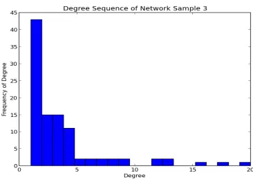
Figure B.9 Spectrum of Network Sample 3 . . . 65
Figure B.10 Degree Multiplicity of Degree Sequence of Network Sample 3 . . . 65
Figure B.11 Spectrum of MCMC Generated Graphs with Degree Sequence
of Network Sample 3 . . . 66
Figure B.12 Zoomed in view of Figure B.11 . . . 66
Figure B.13 Spectrum of Network Sample 4 . . . 67
Figure B.15 Spectrum of MCMC Generated Graphs with Degree Sequence
of Network Sample 4 . . . 68
Chapter 1
Background
1.1 Introduction
The field of complex networks is an exciting area of current study. Having been
a topic of interest since the middle of the last century, the field has very recently
seen a surge in interest from a broad range of disciplines. To help solve important
problems, the field has attracted attention from biologists, physicists, sociologists,
computer scientists, and mathematicians [5]. Thus its development has seen a delicate
interplay between theory and applications. Its beauty lies in its ability to model and
understand real-world phenomenon as well as demonstrate deep theoretical results.
At first glance, a network ultimately is an abstract representation of a set of
dis-crete objects and connections between these objects. In mathematical terms, a
net-work is a graph and thus the objects are referred to as vertices, and the connections
between them are referred to as edges. A network abstracts away from properties of
the underlying system it represents, and captures only topological and connectivity
properties of the system. One of the goals of network science is to understand and
ex-plain properties of a system by the structural connectedness properties of its network
representation. Many scientific phenomenon have very natural representations as
net-works. The internet and world wide web are two of the most studied and prominent
examples of networks. The world wide web is an example of a “directed” network.
Each webpage represents a vertex. Then if pageuhas a hyper-link to another pagev,
mean there is an edge from v to u. Thus the edge is “directed”. Many networks do
not distinguish direction in their edges, and thus, in these cases, two vertices sharing
an edge is not an ordered relationship. We would call this a “simple” network. Other
examples of networks include protein interaction networks, metabolic networks, and
social networks. In a social network, it could be the case that vertices are people and
edges represent relations among the people such as friendship or familial ties. See [3]
for many more examples.
One could claim that graph theory and network science have their origins in the
same story. In 1736, the mathematician Leonard Euler attempted to solve a question
involving bridges in the old city of Königsberg, Prussia. The city lie on the banks of
the Pregel River, and consisted of two islands in the middle of the river. Seven bridges
connected the islands with each other and both sides of the river. The problem was
to determine if there was a path along the network that crosses each bridge exactly
once. The is known as the Königsberg Bridge Problem. This is often cited as the
first problem of graph theory. By abstracting the network of different landmasses
and bridges connecting them to just represent vertices and edges, respectively, the
problem then turns into a graph theoretical question. It turns out that the graph
representing this network does not permit an Eulerian path, which is the correct
mathematical concept to describe the desired path that crosses each bridge exactly
once. Thus by considering this fact, one attains a negative answer to the question. [5]
Figure 1.1 shows the city [13], the network of bridges [31], and graph representation
of this network [32].
Since this time, both fields have been the subject of intense theoretical and
prac-tical study. Barabási et al. present a detailed summary of the field in the book The
Structure and Dynamics of Networks [5]. In this introduction, I present a brief
his-tory of the field along with a discussion of major theoretical developments. Most of
City of Königsberg [13] Bridges of Königsberg [31] Graph representation of bridges of Königsberg [32]
Figure 1.1 Representation of real life problem as a network
invited to consult the book for further details.
In the 1950’s, social scientists saw a need to quantify the methods of their sciences,
such as sociology and anthropology. Thus many adopted terms and concepts from
graph theory to help describe problems they faced. They used these ideas to help
cre-ate models as well as analyze collected empirical data, linking graph theoretical ideas
with social ideas such as “status, influence, cohesiveness, social roles, and identities
in social networks,” [5] page 3. Around the same time, graphs became an accepted
model for means of disease and information transmission. Furthermore, it was around
this time that the notion of random graphs saw its early developments. This new
approach saw graphs as stochastic, or probabilistic, objects rather than deterministic.
All these events thus produced a surge of interest in the new field of network science.
[5] chapter 1. Before any further discussion of the historical development of network
science, it is important to introduce several basic concepts from graph theory. For a
complete introduction to graph theory, see e.g. Diestel’s bookGraph Theory [9].
1.2 Graph Theory
Notation 1.1. Letn ∈N. [n] ={z ∈Z: 1≤z≤n}
Notation 1.2. If V is a set and k is a positive integer, then [V]k is the set of all
Notation 1.3. If V is a set and k is a positive integer, then Vk is the set of all
k-tuples of elements ofV.
Definition 1.4. A simple, non-directed graph Gis a pair of sets (V, E) where V is a
set of objects which we call vertices and E ⊆[V]2, elements of which are referred to
as edges.
Note that we do not allow for more than one edge between any two vertices.
Definition 1.5. A directed graph is a graph G= (V, A), where A ⊆V2.
For this work, we always assume that V is of finite cardinality. If|V|=n, we can
create a bijection between [n] and V and refer to the vertices asvi, wherei∈[n]. We
assume that a graph is non-directed and simple, unless otherwise stated.
Now we introduce several definitions associated with a graph. In the following,
assume G= (V, E) is a graph with n vertices.
Definition 1.6. A vertex v ∈ V is said to be incident upon an edge e ∈ E if
e={v, w} for some w∈V. In words, v is incident upon e if v is an end-vertex of e.
Conversely, e is also said to be incident upon v.
Definition 1.7. A vertex v ∈ V is said to be adjacent to a vertex w ∈ V if they
share an edge, that is, if {v, w} ∈E.
Definition 1.8. Two vertices are said to beneighbors if they are adjacent.
Definition 1.9. Given a vertex v ∈ V, its neighborhood is the set of its neighbors.
We denote it by N(v) ={y∈V :{y, v} ∈E}.
Definition 1.10. Given a vertex v, its degree, denoted by d(v), is the number of
edges that it is incident with, or equivalently the number of vertices it is adjacent
Definition 1.11. Two edges eand f are said to beindependent if they do not share
an end-vertex.
Definition 1.12. Theorder ofGrefers to the number of vertices in G. It is denoted
by|G|:=|V|.
Definition 1.13. Thesize of Grefers to the number of edges in G. It is denoted by
||G||:=|E|.
Definition 1.14. A path in G is a sequence of vertices v0, v1, . . . , vm where m ≥ 0
such that {{vi, vi+1} : 0 ≤ i ≤ m −1} is a set of m different edges of G, and no
vertices are repeated with the exception thatv0 could equal vm. Denote such a path
as a v0−vm path.
Definition 1.15. A cycle is a path P =v0, v1, . . . , vm in which v0 =vm and m >0.
Note that it follows that in a cycle, m ≥3.
Definition 1.16. The length of a path is the number of edges in the path.
Definition 1.17. The girth of Gis the length of the shortest cycle in G.
Definition 1.18. Given two vertices, u and v, their distance is the length of the
shortestu−v path in G.
Definition 1.19. A subsetU ⊆V of vertices is connected if for every pair of vertices
v, w∈U, there exists av−w path in G.
Definition 1.20. A graph G is connected if and only if the entire vertex set V is
connected.
Definition 1.21. A maximally connected set of vertices of a graph is called a
com-ponent. Thus a connected graph has one component.
v1
v2
v3
v4
Figure 1.2 Example Graph
Definition 1.23. Adominating setDis a subset ofV such that every vertex not inD
has at least one neighbor in D. A dominating component is a connected dominating
set.
Definition 1.24. Two graphsG= (V1, E1) and H= (V2, E2) are isomorphicif there
exists a bijection φ:V1 →V2 such that {u, w} ∈E1 if and only if {φ(u), φ(v)} ∈E2.
Definition 1.25. If Ω is a set, then P(Ω) is the set of all subsets of Ω, called its
power set.
Definition 1.26. : Given a graph G on vertex set {v1, . . . , vn}, there exists an
associated degree sequence D. D is the list of non-negative integers (d1, d2, . . . , dn)
such that d(vi) = di.
Figure 1.2 is an example of a graph that has degree sequence (3,3,3,3).
As the order and size of a graph becomes very large, it is often computationally
impractical to obtain exact measurements of graph parameters, such as the diameter,
all graphs on a fixed number of vertices, n, as a probability space. Letting n go to
infinity, one can often obtain average measurements of these parameters in terms of
n. One can obtain a probability measure of the set of graphs on n vertices having
properties of interest. Thus a random graph in this space will have these properties
of interest with this associated probability. Thus it is important to understand some
basic notions from probability.
Modern probability relies on the mathematical axioms, definitions, and results
of set theory and mathematical analysis, specifically measure theory. By rigorously
defining probability spaces, one is able to use powerful tools from analysis. To begin
with, a probability space is a special kind of mathematical object called a measure
space. Several background definitions are needed. Many of the following definitions
are taken from Resnick’s book A Probability Path. See this for further reference [27].
1.3 Probability
Definition 1.27. An experiment is a hypothetical or realistic scenario in which a
range of outcomes are possible.
Examples include rolling a six-sided dice or flipping a two-sided coin.
Definition 1.28. The set of outcomes that can occur in an experiment is referred to
as the sample space. A sample space is typically denoted by Ω. Flipping a coin, the
sample space could be {0,1}where 0 represents a tails and 1 represents a heads.
Definition 1.29. Given an experiment, we can associate probabilities to each
out-come in the sample space. This is called a probability distribution.
Definition 1.30. If Ω is a an arbitrary set, then a set,A, of subsets of Ω is aσ-algebra
on Ω provided that the following conditions hold:
(i) Ω∈ A;
(iii) If C ∈ A, then its complement C0 = Ω−C∈ A.
Condition (ii) is referred to as being closed under countable unions. It quickly
follows from these axioms that∅ ∈Ω, and A is closed under countable intersections.
P(Ω) is a simple example of a σ-algebra on Ω.
Definition 1.31. : A measurable space is a pair (Ω,A) where Ω is a set and A is a
σ-algebra over Ω.
Definition 1.32. Let A be a σ-algebra on a set Ω. A measure on A is a function
µ:A → R∪ {+∞} which obeys the following axioms:
(i) Empty set: µ(∅) = 0;
(ii) Non-negativity: µ(E)≥0 for all E ∈Ω;
(iii) Countable additivity: For a countable collection {Ci}i∈N of pairwise disjoint
elements in Ω, µ(∪∞
i=1Ci) =P∞i=1µ(Ci).
Definition 1.33. A measure space is a triple (Ω,A, µ) where Ω is a set, A is a
σ-algebra of subsets of Ω, andµ is a measure on A.
Definition 1.34. A probability space is a measure space (Ω,A, P) where P(Ω) = 1.
A probability distribution can be thought of as a probability measure on the sample
space.
Definition 1.35. : Given a probability space (Ω,A, P), each element of A is called
anevent.
So if Ω is the set of all possible outcomes of an experiment, an event A∈ A is a
subset of outcomes. We say that the eventAoccurs if the outcome of the experiment
is an element of A.
Definition 1.36. : Given a sample space Ω, a random variable is a measurable
For example, suppose that a two-sided coin is tossed n times. Using the same
encoding as before, let then-tuple (o1, o2, . . . , on) represent a possible outcome of the
n tosses where oi ∈ {0,1} for 1 ≤ i ≤ n. Thus Ω consists of all 2n such n−tuples.
Then the variable X : Ω → {0, . . . , n} is a random variable where X outputs the
number of heads of a given outcome. Given a random variable X and a probability
measure P on Ω, there is an associated probability distribution (measure), D, on
R. That is, for y ∈ R, D(y) = P(X−1(y)). In the example above, supposing each
outcome has an equal probability of 1
2n, D(k) =
(n k)
2n for 0≤k ≤n. Several common
distributions arise frequently and thus are given names. When necessary, we will
define such a distribution.
Definition 1.37. Given a random variable X on a probability space (Ω,A, P), the
expected value of X is defined formally as the Lebesgue integral E[X] =R
ΩXdP. In
the discrete case, this turns out to beP
ixipi wherexi ranges over all possible values
of X and X takes the value ofxi with probability pi.
The expected value of a random variable can be viewed as its average value. Here
we talk about the notion of dependence between events in a probability space, as this
is important in understanding Markov Chains, to be discussed later.
Definition 1.38. IfE, F are events in some sample space Ω withP(F)6= 0, we define
theconditional probability of the eventE occurring given thatF occurs asP(E|F) =
P(E∩F)
P(F) . This can be generalized to an arbitrary number of events. IfA, E1, E2, . . . , En
are events with P(∩n
i=1Ei)6= 0,then P(A|E1, E2, . . . , En) =
P(A∩(∩n i=1Ei))
P(∩n i=1Ei)
is the
prob-ability of A given the occurrence of the eventsE1, . . . , En.
Definition 1.39. : Two eventsE, F in a probability space are said to beindependent
if P(E∩F) = P(E)·P(F). If P(F)6= 0, this is equivalent with P(E|F) =P(E).
Independence is important in understanding random graph processes. As said
combina-torics and graph theory, the asymptotic limiting behavior of a random process is of
most importance. Also, one often speaks of an event occurring with high probability.
We will define this formally.
Definition 1.40. Given some propertyAand a probability space (Ω,A, P), it is said
that A holds almost surely if there exists a set N ∈ A such that P(N) = 0 and for
w∈N0, A holds. Thus A will hold always, except for on a set of probability zero.
Definition 1.41. Given an arbitrary function real-valuledf, limn→∞f(n) =Lmeans
that given an arbitrary >0, there existsN ∈Nsuch that for alln≥N,|f(n)−L|<
. Lis the asymptotic limit of f.
Sometimes, an exact limit of a function is not known. But it is known that its
limiting behavior is similar to that of a simpler function which is better understood.
Thus a function is spoken about with reference to its asymptotic order. Letf(n), g(n)
be two non-negative functions. The following notation is used:
f(n)∈O(g(n)) means that there exists n0 such that for all n≥n0, f(n)≤kg(n)
for some positive constant k.
f(n)∈Ω(g(n)) means that there existsn0 such that for all n≥n0, f(n)≥kg(n)
for some positive constant k.
f(n) ∈ Θ(g(n)) means that there exists n0 such that for all n ≥ n0, k2g(n) ≤
f(n)≤k1g(n) for some positive constants k1, k2.
f(n) ∈ o(g(n)) means that for every > 0, there exists n0 such that for all
n≥n0, f(n)≤g(n).
f(n)∼g(n) means that f(n)−g(n)∈o(g(n)).
1.4 History
Here we will discuss several developments historically important to the field,
develop-ments coming from biologists, sociologists, and mathematicians. Graph theorists are
familiar with the Erdős-Rényi random graph model, introduced by Paul Erdős and
Alfréd Rényi in the 1960 paper, “On The Evolution of Random Graphs” [11]. It is
interesting to note, though, that several of the basic notions were actually introduced
a decade earlier by the biologists Anatol Rapoport and Ray Solomonoff in their 1951
paper, “Connectivity of Random Nets” [29]. Rapoport, one of the earliest
mathemat-ical biologists, was interested in statistmathemat-ical aspects of networks. This was a new notion
at the time, looking at averages over random models rather than individual graphs.
In their paper, they considered a random graph model. They studied the component
structure of networks, and predicted a deep theoretical result proven by Erdős-Rényi,
that is the phase transition of the component structure. Their model is essentially
the same as the Erdős-Rényi model in that it considers a set of vertices with edges
randomly placed between them. For a randomly chosen vertex, they looked at its
ex-pected component size, referred to by them as “weak connectivity”. They concluded
that the weak connectivity is dependent on the mean degree a of the vertices. For
a <1, the network has many small components, but for a >1, a giant, dominating
component arises. This is essentially the phase transition of the component structure
proven rigorously by Erdős-Rényi. The authors suggest several problems for which
their model might be useful. These problems involve neural networks, epidemiology,
and genetics [5], page 11-12.
Erdős and Rényi were not aware of the contributions by Solomonoff and Rapoport
and treated the subject independently of them. Nonetheless, the Erdős-Rényi
treat-ment was mathematically thorough and delved deeper into the subject than their
predecessors. They produced many papers and results involving random graphs over
network science as well as for the purely mathematical topic of probabilistic
com-binatorics, or rather the so-called “probabilistic method”. See Alon and Spencer’s
book The Probabilistic Method for an exhaustive treatment of this subject [2]. This
random graph model is one of the points where network science shares an unclear
boundary with deep theoretical, mathematical results. We will discuss particulars of
this model later when we also introduce several other network models [5], page 12.
One of the most influential sociological papers was put forth in 1978 by the
po-litical scientist Ithiel de Sola Pool and the mathematician Manfred Kochen in their
paper “Contacts and Influence” [8]. The paper concerns social network structure and
patterns. Written in 1958, it was not published until twenty years later because the
authors were not satisfied with the depth of their work. A manuscript was produced
though, and the paper was un-officially circulated amongst the relevant research
com-munity. The paper put forth many of the crucial issues that came to define the field
for some time after. In this network, they treat people as vertices and acquaintances
between two people as an edge. Issues addressed involve an individual person’s
de-gree, degree distributions, average and range of degrees, high-degree people, network
structure, probability of a random acquaintance, probability of shared acquaintances
or neighbors, and shortest path lengths. Due to the insufficiency of empirical data,
they used the random graph model. They were also the first to scientifically
intro-duce the notion of the small-world effect, popularized as “6 degrees of separation”,
which refers to the idea that everybody in the world is within a relatively short social
distance of everybody else [5], page 15.
The scientific community itself also gives rise to several networks. One of these
was first studied by Derek de Solla Price in his 1965 paper “Networks of Scientific
Papers” [24]. In this directed network, each paper is a vertex, and a citation of another
paper is represented by a directed edge from the first to the cited. Each paper has an
namely the distributions of them and discovered that they have power-law tails. This
phenomenon has later been observed in many naturally occurring networks, and a
network with such a degree distribution is referred to as a “scale-free network.” In
1976, he published another paper which proposed an explanation for the existence
of power-laws in certain networks. This explanation has been widely accepted and
adopted and is known today as “preferential attachment” [25]. The explanation claims
that “citations receive further citations in proportion to the number they already
have” [5], page 18. Thus vertices with a large degree are more likely to accumulate
more neighbors. Preferential attachment and scale-free networks are notions of much
interest in network science today [5], page 17-18.
As for the current state of the field, networks have seen a very recent surge in
scientific interest over the last two decades. The most influential reason for this is
probably the advent of the use of computers, the internet, and the world wide web
in everyday society. With this surge, the field has also undergone some changes in
the way research is conducted. Barabási highlights three major points in this change
in [5]. He claims that there is more emphasis on empirical questions than before;
networks are seen as evolving rather than static; and the dynamical structure of the
underlying system on which the network lies is being taken into consideration more,
thus viewing the network no longer as a purely topological object [5], chapter 1.2.
There is now a concerted effort to find accurate models of the empirical networks
at hand. One reason this has not been a practical concern up until now is the
inability to sufficiently collect meaningful data. Obviously, we need the computer
to facilitate this [5], page 4-5. Networks evolve in the real sense that a person’s
number of acquaintances might change over time in a social network, the number of
citations of a paper can change in a citation network, and a web-page can add or
delete hyper-links with time. Thus models capturing time-evolving networks rather
of the system underlying a network, it is important to take real properties of the
network into account. For example, in epidemiology, it should not be assumed that
all people have equal interaction probabilities. Social rules will dynamically affect
the probability of two specific vertices interacting. Corresponding models need to
account for that [5], page 8.
It is important to look at the theoretical models that have been developed and used
over time. Given real networks with certain properties of interest, we want models
that accurately capture these properties. To find such models and then analyze them
from a theoretical standpoint is obviously one of the tasks of network science. We
discuss theoretical properties of several models and highlight where they have fallen
short. [5] highlights three significant models: the Erdős-Rényi random graph, the
small-world model, and the scale-free model.
The Erdős-Rényi random graph model takes two different forms: G(n, p) and
G(n, m). G(n, m) refers to the space of all graphs with n vertices and m edges,
equipped with uniform probability. For 0 ≤ p≤ 1, G(n, p) refers to the space of all
graphs on [n], in which for i, j ∈ [n], Pr[{i, j} ∈ E(G)] = p. For any two possible
edges e, f, the events that e ∈ E(G) and f ∈ E(G) are independent. We will focus
on G(n, p). In this space, each graph has a certain probability which is a function
of n, p, and its size m: pm(1−p)(n2)−m. One is concerned with the behavior of the
space asymptotically, as n → ∞. p is typically treated as a function of n, denoted
p(n), and in this sense we can define threshold functions. Given some graph property
A, one wishes to determine whether there is a threshold function r(n), such that
when r(n) ∈ o(p(n)), the probability that G(n, p) satisfies A goes to 1 and when
p(n)∈o(r(n)), this probability goes to 0. Thus when we say that a certain property
holds in G(n, p) for certainp, we are saying that the property holds almost surely as
n goes to infinity. The most noted result regarding this model is the phase transition
evolution of G(n, p) goes as follows: (1) when p < 1−
n , all components are trees or
unicyclic, having one cycle, and of size ≤ o(ln(n)); (2) when p > 1+n, there exists
a giant component of size Θ(n), and all other components are of size o(ln(n)); (3)
when p = 1+λn
1 3
n for λ a real constant, the largest component has size Θ(n
2 3); (4)
p∼(1 +o(1))ln(nn) is the threshold for G(n, p) being connected [2].
Also of note in this model is that it can be proven that its underlying probabilistic
structure only allows for the existence of one large component. This, as well as the
predicted component framework, is reflected in many real-world networks [5], page
230. The problem with this model though is that it does not accurately reflect degree
distributions. Given a random vertexv, the probability that it has degree k is given
bypk =
n−1
k
pk(1−p)n−k−1, i.e. the binomial distribution. This is because for each
choice ofkneighbors from the remainingn−1 vertices, there is a probability ofpkthat
allk of them are neighbors and a (1−p)n−k−1 probability that the remainingn−k−1
vertices are non-neighbors. Note that the expected value of the degree is (n−1)p.
If a model assumes that the average (or expected) value of the degree is constant,
i.e. p(n) = c
n−1, then as n → ∞, pk →
(pn)ke−pn
k! . Thus the degree distribution of
any vertex v approaches the Poisson distribution as n → ∞. [5] claims that this
distribution is not the degree distribution seen in many empirical networks. This
is an important issue, since the degree distribution significantly affects the network
structure [5], page 233. We discuss random graphs with given degree distributions or
sequences at a further point, as this is directly related to our project.
The small-world model attempts to capture two properties that appear in many
real-world networks. The first of these is the condition that the distance between
two vertices in a network is relatively short. Specifically, the average distance is a
logarithmic function of the order of the network and thus is growing slowly with the
number of vertices in the network. Secondly, the network experiences high clustering,
share a neighbor. A noteworthy fact about this model is that it has some connections
to statistical physics [5], page 286. See Watts and Strogatz for the first appearance
of and further details to this model [33].
The last model of discussion, the scale-free network, has only recently been of
intense interest. A scale-free network is characterized by the fact that its degree
distribution follows a power law. A power law is a function which outputs a power of
the input value. For example, F(k) = k−2 is a power law function. There has been
recent interest in them, because it has been shown that many real-world networks
follow power laws. The random graph and small-world models do not follow power
laws, in their general form, even though the random graph model can be modified
to follow any desired distribution [1]. Thus the need for models which follow power
laws along with their mathematical analysis has arisen. This problem has attracted
attention from some of the most well-known network scientists and mathematicians.
The celebrated first paper on scale-free networks was by Barabási and Albert in 1999,
titled “Emergence of Scaling in Random Networks” [4]. The paper put forth several
ideas. First, they argued that power-law distributions are common among many
networks, evidencing this with the World Wide Web, a network of film actors [33], and
citation networks [26]. Next, they put forth a model with allows for growth and claim
that models of this kind help explain the existence of power-laws [5], page 335. The
explaining properties of such a model are that they grow, continuously adding new
vertices, and that a vertex gains new edges at a rate proportional to its current degree.
This second property is known as preferential attachment in the literature. In the
real world, it makes sense that the aforementioned networks follow these properties.
The model put forth by Barabási and Albert treats the network as a discrete growth
process, in which at each time step a new vertex is added along withmedges incident
with this vertex and already existent vertices randomly chosen proportionally to their
preferential attachment model have been developed since, and give rise to exponents
in the power law varying from 2 to ∞ depending on the parameters of the model,
thus allowing for a good deal of flexibility [5], page 335-337. Barabási and Albert’s
analytical treatment of their model falls short from a mathematical perspective. Thus
Bollobás et al. took on the role of performing such an analysis [6]. They gave a
mathematical confirmation of the results of Barabási and Albert, rigorously defining
the model and proving the main claim of [4]. They later went on to derive new results
as well, such as the calculation of average path lengths between all pairs of vertices
in Barabási-Albert’s model. This is an interesting example in which phenomenon
were predicted heuristically to later be proven mathematically. Likewise, Aiello,
Chung, and Lu [1] devoted attention to random scale-free networks, thus signifying
an effort from the mathematical community to develop theory pertaining to real-world
Chapter 2
Project
2.1 Degree Sequence
Any graph on vertex set {v1, . . . , vn} has an associated degree sequence, i.e. a finite
sequence of integers (d1, . . . , dn) such thatd(vi) = di. The converse is not always true
though: given an arbitrary finite sequence of non-negative integersL, there does not
necessarily exist a simple graph which hasL as its degree sequence. We give a name
to sequences which are the degree sequence of some simple graph.
Definition 2.1. A finite sequenceD of n non-negative integers is called graphical if
there exists a graph on n vertices which has D as its degree sequence. Likewise, we
call such a sequence non-graphical if no such graph exists.
Definition 2.2. If a degree sequence, D, is graphical, we call a realization of D a
graph which has D as its degree sequence.
For example, D = (3,3,1,1) is non-graphical. To see this, assume GD is a
real-ization ofDwith vertex set {v1, v2, v3, v4}. Thenv1 andv2 are attached to all others.
Then since v3 and v4 are adjacent with both v1 and v2, the degree of both is greater
than 1. Thus we have a contradiction and see that D is not graphical.
In general, a realization of a graphical sequence, D = (d1, . . . , dn), is not unique.
LetSD refer to the set of graphs which haveDas its degree sequence. Obviously SD
is finite. Generating all graphs inSD is in general not an easy problem. But once at
least one graph inSD is generated, there is an operation called “switching” (sometimes
v1
v2
v3
v4
v5
Figure 2.1 Switch in which {v1, v4} and {v3, v5} are deleted, and {v1, v5}and
{v3, v4} are added
SD. That is, given a graph G with a prescribed degree sequence D, performing a
“switch” produces a different graph with the same degree sequence, given that G is
not the unique realization ofD. Switching goes as follows:
1. Find two independent edges {u, v},{w, x} such that both {u, w} and {v, x}
are non-edges.
2. Switch end-vertices to produce a graph G0 in which {u, v} and {w, x} are no
longer edges and {u, w}and {v, x} are edges.
Note that all involved vertices maintain the same degree, and thus G0 has the
same degree sequence as G. Thus this operation is closed with respect to the state
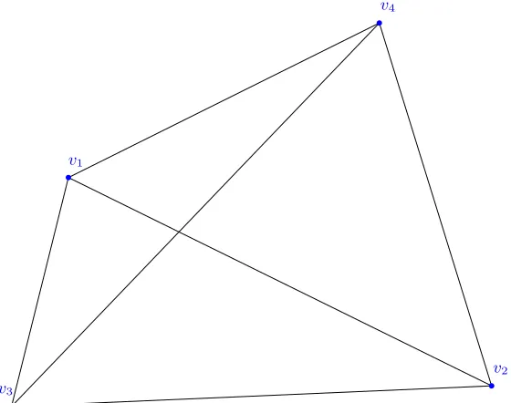
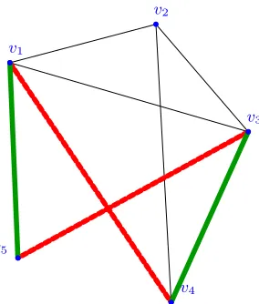
space SD. Figure 2.1 shows an example of a switch.
As stated above, provided that one has a realization, switching allows one to
generate every graph in SD. That is, every realization inSD can be reached by every
other realization inSD by a finite sequence of switches. We prove this below. We can
think of the state space SD as a graph, in which each event (realization) is a vertex,
and there is an edge between two realizations if and only if one can be reached from
the other by one switch. Note that switching is commutative, in that if realizationA
is non-directed. Since there is an A−B path from each realization to every other
realization, we say that this state space is connected with respect to switching.
Lemma 2.3. Given a realizable degree sequence D onn ≤3vertices, the state space
SD is connected with respect to switching.
Proof: Forn= 1,2,and 3,for any degree sequence onnvertices, the corresponding
state space is a single point, and so it is connected.
Claim 2.4. Let G be a graph with degree sequence (d1, d2, . . . , dn) where d1 ≥ d2 ≥
. . . ≥ dn−1, dn > 0. For a graph with such a degree sequence, let its vertex set be
{v1, v2, . . . , vn}, where deg(vi) =di. Let G(G) be the set of graphs that can be realized
from G by a sequence of switches. Then there exists a graph G0 in G(G) such that
NG0(vn) ={v1, v2, . . . , vdn}.
Proof: Clearlydn ≤n−1. If dn=n−1,then NG(vn) = {v1, . . . , vn−1}and so we
are done. So assumedn < n−1. LetG0 ∈ G(G) be such that|NG0(vn)∩{v1, . . . , vdn}|
is maximal. Assume NG0(vn) 6= {v1, . . . , vdn}. Let i be the smallest index such
that vi ∈/ NG0(vn). There exists j > dn such that vjvn ∈ E(G0). Now note that
i < j implies that di ≥ dj. Since vn ∈ NG0(vj)\NG0(vi), there must exist some
k /∈ {i, j, n} such that vk ∈ NG0(vi) \ NG0(vj). Then {vi, vk},{vn, vj} ∈ E(G0)
while {vi, vn},{vk, vj}∈/ E(G0). So we can perform a switch, making vi ∈ NG0(vn),
contradicting the maximality of G0. Thus the claim is proven.
Lemma 2.5. Given a realizable degree sequence D on n vertices, the state space SD
is connected with respect to switching.
Proof: The proof goes by induction on n. By Lemma 2.3, we know the statement
holds forn = 1,2,and 3. These serve as the base cases. So now assume the statement
holds for any graph on n − 1 vertices. Let D = (d1, d2, . . . , dn) be a realizable
LetG, H ∈SD. Ifdn = 0, thenvnis isolated in both Gand H.DefineG∗ =G\ {vn}
and H∗ =H\ {vn}. By the inductive hypothesis, there exists a sequence of switches
from G∗ to H∗ that is also a sequence of switches from G to H. In this case, we
are done. So assume dn > 0. By Claim 2.4, we know that there exists a graph
G0 ∈SD such thatNG0(vn) = {v1, . . . vdn}, and there exists a sequenceS1 of switches
that take G to G0. Likewise, there is such a graph H0 with the same property,
and there exists a sequence S3 of switches that take H to H0. Now observe that
NG0(vn) =NH0(vn) = {v1, . . . , vdn}. This if we remove vn from both G0 and H0, we
remove the same edges from both, that is{vn, vi}for 1 ≤i≤dn. Then bothG0\{vn}
andH0\{vn}have the same degree sequencesd1−1, d2−1, . . . , ddn−1, ddn+1, . . . , dn−1.
So by the induction hypothesis, there exists a sequence of switchesS2 fromG0\ {vn}
toH0\ {vn}. Note that the switches in S2 are also switches fromG0 toH0 since the
switches do not involve any edges with vn as an end-vertex. LetS30 be the reversal of
S3. ThenS1S2S30 is a sequence of switches fromGtoH. SinceGandH are arbitrary,
we see thatSD is connected. SinceDis arbitrary, we see that for any degree sequence
on n vertices, its state space is connected. By induction, the statement holds for all
n∈N.
A natural question involving degree sequences is how to determine whether a
given finite sequence of non-negative integers, L, is graphical or not. Call this the
Graphicality Problem. One quick way to attain a negative answer to this question
relies on one of the most fundamental theorems of graph theory:
Lemma 2.6. (Handshaking [9]) - The sum of the degrees of the vertices of G equals
twice the size of G and thus is always even. Notationally, P
v∈V(G)deg(v) = 2· |E|.
So if the sum of the elements of L is odd, L must be non-graphical. A more
substantial answer to the Graphicality Problem is given by the Erdős-Gallai theorem
which uses this fact plus an extra condition to establish a complete characterization
Theorem 2.7. (Erdős-Gallai [10]) A sequence of non-negative integersd1 ≥. . .≥dn
is graphical if and only if Pn
i=1di is even and Pki=1di ≤k(k−1) +Pni=k+1min(di, k)
holds for 1≤k ≤n.
This theorem answers the Graphicality problem. It does not provide a concrete
realization in the affirmative case though. The Havel-Hakimi Theorem provides a
simple algorithm to determine whether a sequence is graphical, and in the affirmative
case actually produces a realization of the prescribed degree sequence. The proof was
given independently by Havel in 1955 [15] and Hakimi in 1962 [14].
Theorem 2.8. (Havel-Hakimi) A sequence of integers d1 ≥ d2 ≥ . . . ≥ dn > 0 is
graphical if and only if (d2−1, d3−1, . . . , dd1+1−1, dd1+2, dd1+3, . . . , dn) is graphical.
Proof: This is a quick corollary of Claim 2.4 (we need to renumber vertices).
As stated, if the sequence is graphical, this theorem provides an iterative algorithm
to produce a realization. The algorithm follows the following steps:
1. Start with an empty graph, G, and a dictionary L of n vertices as the keys
and a residual degree requirement assigned as the values. The starting list of residual
values will be the degree sequence.
2. If all residual degrees are zero, output G and stop. If any residual degree is
less than 0, output FAILURE and stop.
3. Maintain the dictionary in non-increasing order according to the residual degree
values.
4. Assume the first vertex in the dictionary has a degree requirement ofd. For the
nextd vertices in the list, attach an edge between each vertex and the first vertex.
5. Remove the first vertex from the dictionary and decrease the degree requirement
of these nextd vertices by 1.
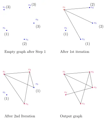
(3) (3) (3) (2) (1) (2) (2) (1) (1)
Empty graph after Step 1 After 1st iteration
v1
v2
v3
v4
v5
v1 v2
v3
v4
v5
(1)
(1)
After 2nd Iteration Output graph
v1
v2
v3
v4
v5
v1 v2
v3
v4
v5
Figure 2.2 Iterations of Havel-Hakimi algorithm for degree sequence (3,3,3,2,1)
Figure 2.2 shows the graphs that are produced after each iteration of the
Havel-Hakimi algorithm when (3,3,3,2,1) is the input degree sequence. The numbers in
parentheses next to the vertices represent the residual degree requirement of the
corresponding vertex after that iteration.
When dealing with SD for a given D, it is natural to ask how many graphs are
realized by this sequence and thus lie in this space. We can easily characterize when
this space only has one graph. Note that for everyn ∈N, there is a uniquely realizable
sequence. The complete graph on n vertices provides a trivial example. There is a
way to characterize all such uniquely realizable graphs.
Define a graph G to be a threshold graph if for every vertex x, y ∈V(G), N(x)⊆
N(y)\ {x}orN(y)⊆N(x)\ {y}. The name of threshold graphs comes from the fact
that they can also be obtained as follows: assign non-negative weights to vertices and
set a threshold T. Let {i, j} ∈E(G) if and only ifw(i) +w(j)> T.
Lemma 2.9. Threshold graphs are precisely those that are uniquely realizable.
Proof: Suppose that a graphGis not a threshold graph. Then there isx, y ∈V(G)
such that neither N(x)6⊆N(y)\ {x} nor N(y)6⊆N(x)\ {y}. Then neither x nor y
is isolated, and there exists a vertex w∈N(x)\N(y) and a vertex v ∈N(y)\N(x).
This means that {x, w},{v, y} ∈ E(G) and {x, v},{y, w} ∈/ E(G); also x 6= v and
y 6= w. Thus we can perform a switch from {x, w} and {y, v} to {x, v} and {y, w},
making a new graph with the same degree sequence. So Gis not uniquely realizable.
On the other hand, suppose that G is a threshold graph. Let {x, w} and {y, v}
be two independent edges in G. Since N(x)⊆N(y)\ {x} orN(y)⊆N(x)\ {y}, we
havev ∈N(x)\ {y} orw∈N(y)\ {x}. In either case, a switch from these two edges
is not permitted. Since these are arbitrary independent edges, we see that no switch
is permitted and thus Gis uniquely realizable.
Thus we may speak of uniquely realizable graphs in terms of threshold graphs.
We make several claims.
Claim 2.10. Let I be the set of isolated vertices of the graph G. G is a threshold
graph if and only if G\I is a threshold graph.
This is self-evident.
Claim 2.11. If G is a threshold graph and contains no isolated vertices, then there
Proof: Letxbe a vertex of maximal degree inG. Suppose thatd(x)<|V(G)| −1,
i.e. N(x)6=V(G)\ {x}. Then there exists a vertexysuch thaty /∈N(x)∪ {x}. Since
there are no isolated vertices, there is an edge {y, z} in G for some vertex z 6= x.
SinceG is a threshold graph, eitherN(z)⊆N(x)\ {z} orN(x)⊆N(z)\ {x}. Since
y ∈ N(z)\N(x), N(z) 6⊆N(x)\ {z}. Suppose N(x)⊆ N(z)\ {x}. Then |N(x)| ≤
|N(z)|. Then since the degree of xis maximal,|N(x)|=|N(z)|which further implies
that N(x) =N(z). But y ∈N(z), andy /∈N(x), which is a contradiction. Thus we
see thatN(x) = V(G)\ {x}.
From the previous two claims and the definition, the following claim follows:
Claim 2.12. If G is a graph and x is adjacent with every other vertex in the graph,
then G is a threshold graph if and only if G\ {x} is a threshold graph.
Thus from these three claims, we have an iterative algorithm to check whether a
graph Gis uniquely realizable or not:
1. Delete all isolated vertices. If the remaining graph is empty, stop and output
that G is a threshold graph.
2. Search for a vertex that is adjacent with every other vertex. If not found, then
stop and output that G is not uniquely realizable. If found, then delete that vertex
and all its incident edges. Go back to Step 1.
This characterizes situations in which the state space consists of a single graph.
There are several results regarding the enumeration of graphs with certain degree
sequences. Linyuan Lu and László Székely apply the Lovász Local Lemma to the
space of random multi-graphs with a given degree sequence to obtain asymptotic
enumeration results in [19]. See [2] for an overview of the Lovász Local Lemma, a
celebrated tool in the probabilistic method. They also outline a brief history of results
involving enumeration of d-regular graphs, that is graphs in which every vertex has
degree d. They attribute the strongest result to McKay and Wormald (strongest in
following best asymptotic boundary on the regularity d. Let (N −1)!! = N!
N/2)!2N/2
for N even. They show that the number of simple graphs in which all vertices have
degree d ford∈o(n1/2) is
(1 +o(1))e1−d
2 4 −
d3
12n+O( d2
n)(dn−1)!!
(d!)n .
Lu and Székely first state a result involving d-regular graphs and then generalize
to a larger class of degree sequences. We state the generalization here. Let xi be real
numbers and assume xi >0 for each i∈[n] for some n∈ N. Define x= (Pni=1xi)/n
and ˜x= (Pn
i=1x2i)/x.
Theorem 2.13. Let di ∈ N for i ∈ [n]. Assume N = d1 +d2 +. . .+dn is even,
d≥3, and every di ≥2. Let Di =di(di−1). Then the number of graphs with degree
sequence d1, d2, . . . , dn and girth g ≥3 is
(1 +o(1))(NQ−1)!!
idi!
exp(−
g−1 X
i=1 1 2i(
D d) i) assuming that (g 2 n + g2 n2 ˜ D d)( D d) g−1
=o(1)
and
g6(D
d)
2g−4
d2n=o(N).
This is the state of the art with respect to the enumeration of graphs with general
degree sequences.
There has been significant attention devoted to random generation of graphs with
given degree distributions, a task of importance to network science. Much significant
work has been done by treating degree sequences rather than distributions. This
distinction is not problematic though in that they correspond to each other: one
determines the other. Since the Havel-Hakimi algorithm produces a graph inSD and
we theoretically can attain every other graph inSD by switches, these methods serve
we generate a realization, G, of D via the Havel-Hakimi algorithm. We then run a
Monte-Carlo Markov Chain on SD with starting point GD via the use of switches.
2.2 Markov Chains
The following definitions are taken from [16], chapters 1,2, and 3. A Markov chain
is a specific kind of probabilistic model. It is an example of a more general notion
called a stochastic process.
Definition 2.14. A stochastic process is a family of random variables defined on
some sample space Ω.
For our purposes, there is a countable number of random variables, and so we
enumerate them asX0, X1, X2, X3, . . .. Intuitively, the indices of the random variables
refer to the time-step of the process. When we say that the process lies in statei at
the nth step, we really mean that Xn takes on the value i. This is called a
discrete-time process. We define the state space of the stochastic process as the union of the
possible values of the individual random variables.
Definition 2.15. A Markov chain, C, consisting of the random variables {Xk}, k =
0,1,2, . . . with state space S is a stochastic process that satisfies the following
prop-erties:
1. It is a discrete-time process.
2. S is countable or finite.
3. Markov property: If for everymand all statesi1, i2, . . . , imwhereij is a possible
value ofXj, it is true that
P(Xm =im|Xm−1 =im−1, Xm−2 =im−2, . . . , X1 =i1) =P(Xm =im|Xm−1 =im−1)
In words, the proximate value of a random variable at a point in time only depends
on its current value and does not depend on previous values in the process. The
process is “memoryless.” Intuitively, a Markov chain travels along a state space. We
will only work with finite state spaces, so we may say S = [N] for some N ∈ N. At
the state space with a given probability. The factors determining the movement of a
Markov chain are governed by the set of conditional probabilities
P(Xm =j|Xm−1 =k)
for every pair of statesk, j in the state space. We can also refer to these as transitional
probabilities at timem. We can further classify these processes according to whether
these conditional probabilities are time-dependent or not.
Definition 2.16. A Markov chain ishomogeneousin time if the transition probability
from any given state to any other given state is independent of the time-step. That
is, for arbitrary m and every pair j, i∈S,
P(Xm =j|Xm−1 =i) =P(Xm+k=j|Xm−1+k =i)
for all k such that−(n−1)≤k.
The Markov Chain we use is finite and homogeneous. Set N = |S|. We can
describe the transition probabilities by anN×N transition matrix,T = (pi,j), where
pi,j =P[X1 =j|X0 =i] =P(Xm+1 =j|Xm =i).
It follows from this definition that
1 = P[X1 ∈[N]|X0 =i] =
N
X
j=1
pi,j.
The transition matrix serves as a very useful tool in understanding a Markov chain.
In fact, the analysis of a Markov chain can often be done completely by looking at
its transition matrix. One might ask what is the probability that the chain lies in a
given state at a given time. Transition matrices aid in answering this question.
First, given a current state at timek, the transition matrix can be used to calculate
the probability of being in all other states after m steps for m≥1. This probability
is given by Tm. The entry Tm
that we have some information about the starting point in the chain, specifically we
have a probability distribution for X0. We may encode this information as a vector
α0 = (p1, p2, . . . , pN) wherepi refers to the probability thatX0 is in statei. Note that
this allows for a deterministic or non-deterministic starting point. If deterministic,
then we assign a probability of 1 to its determined value in α0 and a probability of 0
everywhere else. It turns out thatT and α0 is all that is needed to give a probability
distribution for the state of C at a certain time, or rather a probability distribution
of Xm. Letαm =α0 ·Tm. Then αm gives this probability distribution. That is, αmi
gives the probability that C lies in state i at the mth step given the starting vector
α0. Note that this is not a contradiction of being homogeneous. The distinction is
that the probabilities of transitioning from a specific state to another do not change
with time, but rather the probability that C lies in a certain state do change with
time. Often, one is not interested in the behavior of a Markov chain,C, at a specific
point in time but rather interested in its long-term behavior. Does αm converge as
m→ ∞? Some Markov chains do have this property while some do not.
Definition 2.17. Stateiisaccessiblefrom statej if Pr(Xn =i|X0 =j)>0 for some
n∈N.
Definition 2.18. Statei and j communicate if statei is accessible from state j and
state j is accessible from state i.
Definition 2.19. A Markov chain is said to be irreducible if for every pair of states
i < j, iand j communicate.
Using the language we used above with the degree sequence, this is the same as
saying that the state space is connected.
Definition 2.20. The period, R, of a state i is defined as
where gcdis the greatest common denominator.
Definition 2.21. A state i is said to be aperiodic if its period is 1.
Definition 2.22. A Markov chain is said to beaperiodic if each state is aperiodic.
Definition 2.23. A vectorπthat satisfiesπ=π·T is called asteady-state distribution
of C.
Theorem 2.24. A time-homogeneous, irreducible and aperiodic Markov chain with
a finite state space has a unique steady-state distribution.
Note that for a time-homogeneous, irreducible and aperiodic Markov chain, π =
limm→∞α0·Tm for any initial distribution α0, i.e. the chain converges to the
steady-state distribution regardless of the initial distribution.
Definition 2.25. Suppose a Markov Chain, C, converges to a steady-state
distribu-tionπ. Then themixing timetofC is the minimumtsuch that|Pr(Xm =i)−π(i)| ≤
1/4 for all m ≥t and all statesi in the sate space.
Intuitively, the mixing time refers to how many steps are necessary to get
suffi-ciently close to the steady-state distribution. Before we describe our project exactly,
it is important to give an introduction to one more theoretical concept, that is spectral
graph theory.
The Markov Chain we use will have state space SD for some realizable degree
sequence D. The steps of the chain will be defined as follows: Given D, X0 = H,
whereHis created by the Havel-Hakimi algorithm. The transition steps will be
time-independent (thus, the chain is homogeneous); and each step will be defined either
as a switch or staying in place, i.e. P(Xm+1 =G0|Xm =G)>0 if and only ifG0 =G
orG0 can be reached from G by a single switch. We will describe these probabilities