Color Separation for Background Subtraction

Western University Western University

Scholarship@Western

Scholarship@Western

Electronic Thesis and Dissertation Repository

12-6-2016 12:00 AM

Color Separation for Background Subtraction

Color Separation for Background Subtraction

Jiaqi Zhou

The University of Western Ontario Supervisor

Olga Veksler

The University of Western Ontario Graduate Program in Computer Science

A thesis submitted in partial fulfillment of the requirements for the degree in Master of Science © Jiaqi Zhou 2016

Follow this and additional works at: https://ir.lib.uwo.ca/etd Part of the Other Computer Sciences Commons

Recommended Citation Recommended Citation

Zhou, Jiaqi, "Color Separation for Background Subtraction" (2016). Electronic Thesis and Dissertation Repository. 4272.

https://ir.lib.uwo.ca/etd/4272

This Dissertation/Thesis is brought to you for free and open access by Scholarship@Western. It has been accepted for inclusion in Electronic Thesis and Dissertation Repository by an authorized administrator of

Background subtraction is a vital step in many computer vision systems. In background subtraction, one is given two (or more) frames of a video sequence taken with a still camera. Due to the stationarity of the camera, any color change in the scene is mainly due to the pres-ence of moving objects. The goal of background subtraction is to separate the moving objects (also called the foreground) from the stationary background. Many background subtraction ap-proaches have been proposed over the years. They are usually composed of two distinct stages, background modeling and foreground detection.

Most of the standard background subtraction techniques focus on the background modeling. In the thesis, we focus on the improvement of foreground detection performance. We formulate the background subtraction as a pixel labeling problem, where the goal is to assign each image pixel either a foreground or background labels. We solve the pixel labeling problem using a principled energy minimization framework. We design an energy function composed of three terms: the data, smoothness, and color separation terms. The data term is based on motion information between image frames. The smoothness term encourages the foreground and background regions to have spatially coherent boundaries. These two terms have been used for background subtraction before. The main contribution of this thesis is the introduction of a new color separation term into the energy function for background subtraction. This term models the fact that the foreground and background regions tend to have different colors. Thus, introducing a color separation term encourages foreground and background regions not to share the same colors. Color separation term can help to correct the mistakes made due to the data term when the motion information is not entirely reliable. We model color separation term with L1 distance, using the technique developed by Tang et.al. Color clustering is used to efficiently model the color space. Our energy function can be globally and efficiently optimized with graph cuts, which is a very effective method for solving binary energy minimization problems arising in computer vision.

To prove the effectiveness of including the color separation term into the energy function for background subtraction, we conduct experiments on standard datasets. Our model depends on color clustering and background modeling. There are many possible ways to perform color clustering and background modeling. We evaluate several different combinations of popular color clustering and background modeling approaches. We find that incorporating spatial and motion information as part of the color clustering process can further improve the results. The best performance of our approach is 97% compared to the approach without color separation that achieves 90%.

Keywords: background subtraction, graph cuts, color separation, energy optimization

Acknowledgements

I would like to express my deepest gratitude to my supervisor, Dr. Olga Veksler, who gave me great help by providing me with necessary materials, advice of great value and inspiration of new ideas. She walked me through all the stages of the writing of this thesis. It is her suggestions that draw my attention to a number of deficiencies and make many things clearer. Without her strong support, this thesis could not been the present form.

I would like to express my sincere thanks to Dr. Yuri Boykov, whose lectures have a great influence on my study in computer vision and image analysis. I feel grateful that I had the change to attend his lectures. The clear and detailed ways he explained a problem impressed me a lot.

Special thanks are given to the members of my examining committee, Dr. John Barron, Dr. Robert Mercer and Dr. Jagath Samarabandu.

I would like to thank Dr. Lena Gorelick for her valuable and helpful suggestions to my thesis. She taught me how to explain a problem in a more comprehensive way.

I also owe my heartfelt gratitude to my friends and other members in our vision group, who gave me their help and time in listening to me and helping me work out my problems during the difficult course of the thesis. I want to give special thanks to Meng Tang who did the prior work of this thesis. He answered my questions patiently when I came to him for help.

I would extend my thanks to the help and support of the staffmembers in the main office and system group.

I especially appreciate the support of my parents, who give me continuous encouragement and love through all these years.

Abstract i

Acknowledgements ii

List of Figures v

List of Tables ix

1 Introduction 1

1.1 Background Subtraction . . . 1

1.2 Our Approach . . . 4

1.3 Outline of the Thesis . . . 8

2 Background Subtraction Techniques 9 2.1 Basic Models . . . 9

2.1.1 Static Frame Difference . . . 9

2.1.2 Further Frame Difference . . . 10

2.1.3 Mean Filter . . . 12

2.2 Gaussian Average . . . 12

2.3 Gaussian Mixture Model . . . 14

3 Image Segmentation Techniques 17 3.1 Kmeans . . . 17

3.2 Mean Shift . . . 18

3.3 Efficient Graph-based Image Segmentation . . . 21

3.3.1 Graph-based segmentation . . . 21

3.3.2 Pairwise region comparison metric . . . 21

3.3.3 Algorithm . . . 22

4 Energy Minimization using Graph Cuts 25 4.1 Labeling Problem and Energy Minimization Framework . . . 25

4.2 Optimization with Graph Cuts . . . 27

4.3 Color Separation Term . . . 32

5 Background Subtraction using Color Separation Term 37 5.1 Overview . . . 38

5.2 Graph Construction for Energy Function . . . 43

5.2.1 Data Term . . . 44

5.2.2 Color Separation Term . . . 46

5.2.3 Smoothness Term . . . 48

6 Experimental Results 51 6.1 Image Database . . . 51

6.2 Parameter Selection . . . 52

Parameters in Kmeans . . . 52

Parameters in Meanshift . . . 53

Parameters in Efficient Graph-based Image Segmentation Algorithm . . 53

Parameters in Energy Function . . . 54

6.3 Evaluation Methods . . . 55

6.4 Evaluation of the Results . . . 57

Results without Color Separation and without Motion Information . . . 57

Results with Color Separation and without Motion Information . . . 57

Results with Color Separation and with Motion Information . . . 59

6.5 Results Comparison . . . 59

Background Modeling Techniques Comparison . . . 60

Comparison with Color Separation . . . 62

Comparision with Motion Information . . . 62

6.6 Failure Cases . . . 67

7 Conclusion and Future Work 68

Bibliography 69

Curriculum Vitae 71

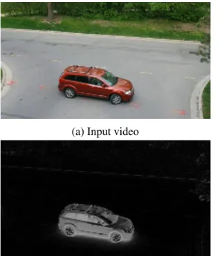
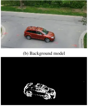
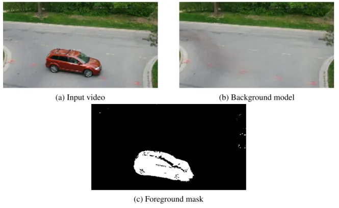
1.1 Example of input to the background subtraction algorithm. The background model is estimated from the scene without moving objects, as shown in (b). Usually, more than one frame is used for estimating the background model, to be robust to illumination changes. Given a new, previously unobserved frame (a), the task is to find pixels that belong to the new object (the red car in this case). It is done by thresholding the difference between the current frame and the background model, as shown in (c). The foreground detection results with

different thresholds 15, 25, 40 are shown in (d), (e), (f) separately. . . 2

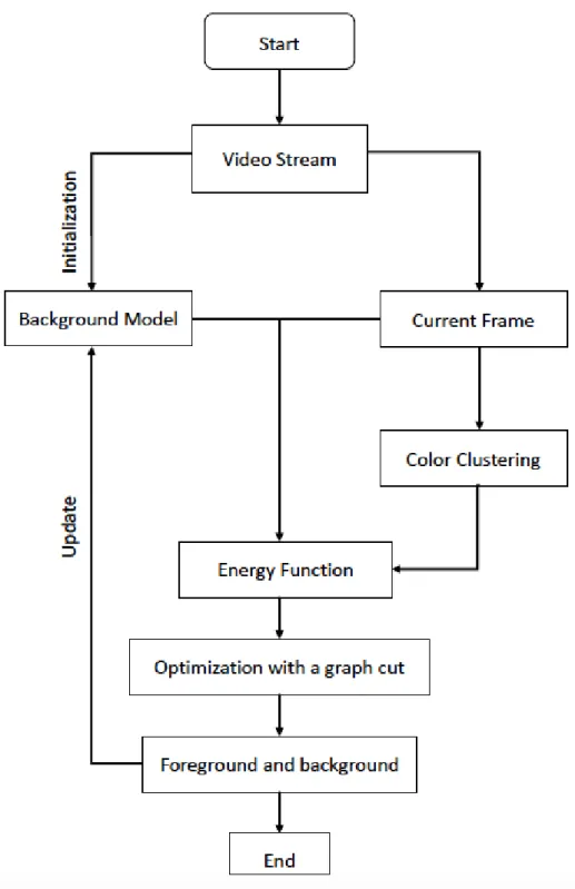
1.2 The flow chart of the algorithm . . . 6

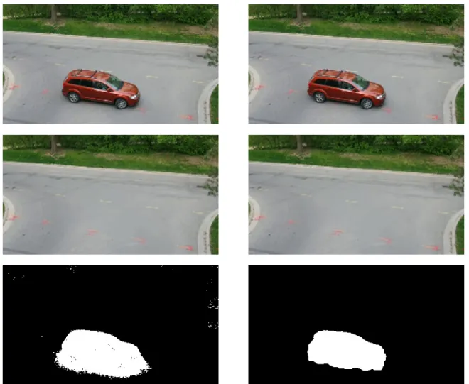
1.3 Example of background subtraction results using GMM (left) and our algo-rithm (right): (top) original image; (middle) background model; (bottom) fore-ground mask. . . 7

2.1 Background subtraction using static frame difference . . . 10

2.2 Background subtraction using further frame. We chose the threshold that leads to the best result. . . 11

2.3 Background subtraction using mean filter . . . 13

2.4 Background subtraction using Gaussian average . . . 14

2.5 Background subtraction using Gaussian mixture model . . . 16

3.1 Example of mean shift for 1D histogram . . . 19

3.2 Example of mean shift segmentation with different color features: (a) Ori-gianl image, (b)-(g) mean shift segmentation using scale bandwidth 7 and color bandwidths 3, 7, 11, 15, 19 and 23 respectively. [28] . . . 20

3.3 A synthetic image (320×240 grey image), and the segmentation results (σ = 0.8,k=300) [11]. . . 23

3.4 A street scene (320× 240 color image), and the segmentation results (σ = 0.8,k=300) [11]. . . 23

3.5 A baseball scene (432×294 grey image), and the segmentation results (σ = 0.8,k=300) [11]. . . 23

4.1 Illustration of 4 and 8 neighborhood systems in images . . . 27

4.2 An example of a graph with source and sink terminals. [Image credit: Yuri Boykov] . . . 28

4.3 An example of as−tcut on a graph. [Image credit: Yuri Boykov] . . . 29

4.5 Binary segmentation for 3 by 3 image. (top-left): Original image; (top-right): Graph constructed based on original image with source and sink terminals; (bottom-right) A minimum cut for the graph separating all pixels into two dis-joint sets; (bottom left): Segmentation result, one color stands for one label. [Image credit: Yuri Boykov] . . . 31 4.6 Color separation gives segments with low entropy. [Image credit: Meng Tang] . 33 4.7 Plots for different energy terms. . . 34 4.8 Graph construction forL1color separation term in one color bin. [Image credit:

Meng Tang] . . . 34 4.9 Overall graph construction for energy withL1 color separation term. This

ex-ample shows three different color bins, blue, orange and green. Three auxiliary nodes are added for these color bins. All pixels are connected to the corre-sponding auxiliary node. [Image credit: Meng Tang] . . . 35 4.10 Example of segmentation results with one graph cut. [Image credit: Meng Tang] 36

5.1 The flow chart of the algorithm . . . 39 5.2 An example of background subtraction using Gaussian average model: a

se-quence of images from a video stream (first row and third row) and corre-sponding background subtraction results (second row and last row). . . 40 5.3 Illustrates motion information using the mean filter background modeling. . . . 41 5.4 An example of the foreground mask (left) and background mask (right) using

mean filter. White area in the two images represents the pixels that prefer to be foreground and background respectively. . . 41 5.5 Color clustering results using different algorithms. . . 42 5.6 An example of the visualization of edge contrast between neighboring pixels. . 43 5.7 An example of color clustering results using the efficient graph-based

segmen-tation algorithm. . . 44 5.8 Overall graph construction for energy withL1 color separation term. . . 50

6.1 Sample frames (top) and the corresponding ground truth (bottom) from our dataset: (a) a general sequence from object detection dataset used in [7], (b)-(c) sequences from wallflower dataset [32], (d) sequence obtained by ourselves. 52 6.2 Example of kmeans clustering results with different number of clusters: (a)

original image, (b)-(g) kmeans color clustering with number of clusters 3, 5, 8, 10, 15, 20 and 50 respectively. . . 53 6.3 Example of meanshift clustering results with different color bandwidths: (a)

original image, (b)-(g) mean shift clustering using scale bandwidth 10 and color bandwidths 3, 5, 6, 6.5, 8 and 10 respectively. . . 54 6.4 Example of an efficient graph-based clustering results with different color

fea-tures: (a) Original image, (b)-(g) graph-based clustering using cluster threshold 100, 150, 200, 300, 500, 1000 and 1500 respectively. . . 54 6.5 Example of background subtraction results with different weight of

smooth-ness term using mean filter background modeling techniques without the color separation term: (a) original image, (b)-(d) background subtraction results with

information: (a) original image, (b)-(d) background subtraction results with

λ= 50 andβ=1, 10, 100, 200, 1000 respectively. . . 56 6.7 Background subtraction results on an indoor scene with different background

modeling techniques without color separation term. First column shows the original image (top) and the corresponding ground truth (bottom). The second column is the data term mask (top) and background subtraction result (botton) using mean filter background modeling technique. Red is the foreground and blue is the background masks for the background modeling step. The third column is the data term mask (top) and background subtraction result (bottom) using Gaussian average background modeling technique. The fourth column is the data term mask (top) and background subtraction result (bottom) using Gaussian mixture model background modeling technique. . . 60

6.8 Background subtraction results on a moving person scene with different back-ground modeling techniques without color separation term. First column shows the original image (top) and the corresponding ground truth (bottom). The second column is the dataterm mask (top) and background subtraction result (bottom) using mean filter background modeling technique. Red is the pri-ori foreground information from the background modeling process and blue is the priori background information. The third column is the dataterm mask (top) and background subtraction result (bottom) using Gaussian average back-ground modeling technique. The fourth column is the dataterm mask (top) and background subtraction result (bottom) using Gaussian mixture model back-ground modeling technique. . . 61

6.9 Background subtraction results on a waving tree scene with different back-ground modeling techniques without color separation term. First column shows the original image (top) and the corresponding ground truth (bottom). The second column is the dataterm mask (top) and background subtraction result (bottom) using mean filter background modeling technique. Red is the pri-ori foreground information from the background modeling process and blue is the priori background information. The third column is the dataterm mask (top) and background subtraction result (bottom) using Gaussian average back-ground modeling technique. The fourth column is the dataterm mask (top) and background subtraction result (bottom) using Gaussian mixture model back-ground modeling technique. . . 61

6.10 An example of background subtraction results on an indoor scene with dif-ferent combinations of background modeling techniques and color clustering algorithms. Left: background subtraction method using mean filter. Middle: background subtraction method using Gaussian average. Right: background subtraction method using Gaussian mixture model. From top to bottom are background subtraction methods: without color separation, with kmeans color clustering algorithm, with meanshift color clustering algorithm and with effi -cient graph-based color clustering algorithm. . . 63

6.11 An example of background subtraction results on a waving tree scene with dif-ferent color clustering algorithms using Gaussian average background model-ing technique. (a) original image, (b) ground truth, (c) background subtraction result without color separation, (d) background subtraction result with kmeans color clustering, (e) background subtraction result with meanshift color cluster-ing, (f) background subtraction result with efficient graph-based color clustering. 64 6.12 An example of background subtraction results on an indoor scene with diff

er-ent background modeling techniques using kmeans color clustering algorithms with motion information. Left: background subtraction method using mean filter. Middle: background subtraction method using Gaussian average. Right: background subtraction method using Gaussian mixture model. From top to bottom are background subtraction methods: without color separation, with kmeans color clustering algorithm without motion, with kmeans color cluster-ing algorithm with motion. . . 65 6.13 An example of background subtraction results on an indoor scene with diff

er-ent background modeling techniques using efficient graph-based color cluster-ing algorithms with motion information. Left: background subtraction method using mean filter. Middle: background subtraction method using Gaussian av-erage. Right: background subtraction method using Gaussian mixture model. From top to bottom are background subtraction methods: without color sep-aration, with efficient graph-based color clustering algorithm without motion, with efficient graph-based color clustering algorithm with motion. . . 66 6.14 An example of background subtraction results on a waving tree scene using

Gaussian average background modeling method with two color clustering al-gorithms including motion information. From left to right are background sub-traction methods: without color separation, with color clustering algorithm without motion, with clustering algorithm with motion. Top: with kmeans color clustering algorithm. Bottom: with efficient graph-based color clustering algorithm. . . 67

6.1 Average error rate, recall, precision and F-measure of different methods in backgound modeling. . . 57 6.2 Average error rate, recall, precision and F-measure of different backgound

modeling techniques using kmeans color clustering. This table shows the ef-fectiveness of color separation. . . 58 6.3 Average error rate, recall, precision and F-measure of different backgound

modeling techniques using meanshift color clustering. This table shows the effectiveness of color separation. . . 58 6.4 Average error rate, recall, precision and F-measure of different backgound

modeling techniques using an efficient graph-based color clustering. This table shows the effectiveness of color separation. . . 58 6.5 Average error rate, recall, precision and F-measure of different backgound

modeling techniques using kmeans color clustering with motion information. This table shows the benefits of motion information. . . 59 6.6 Average error rate, recall, precision and F-measure of different backgound

modeling techniques using an efficient graph-based color clustering with mo-tion informamo-tion. This table shows the benefits of momo-tion informamo-tion. . . 59

Chapter 1

Introduction

1.1

Background Subtraction

Background subtraction is a vital step in many computer vision applications and it is mainly used for detecting moving objects in videos from static cameras. The rationale of this approach is to segment out foreground objects from their background in a video sequence by using the difference between the current image and a background image (see Figure 1.1). Here the background image represents the scene without moving objects. Background subtraction is composed of two distict steps, background modeling and foreground detection. These two steps are performed successively. In the background modeling, a background model is estimated in the beginning of the algorithm and usually it is updated regularly during the deployment of the algorithm. The need to update the background is due to multiple factors. For example, the illumination in the scene may change due to the change in the weather conditions, or due to the change in time of the day. Also, if an object was moving but then stops moving for a sufficient long time (for example a car that has been parked), then it should be considered as part of the background. Thus a reliable background model should adapt with time to the changing circumstances in the scene. In foreground detection, a decision is made about whether a pixel fits the background model or not. The result is ususlly fed back to background modeling, so that no foreground pixels are used when constructing the background model.

Many background subtraction approaches have been proposed previously. The simplest way to build a background model it to manually select a static image that represents the back-ground and has no moving object. By thresholding the difference between the current image and the chosen image, the foreground can be detected, as shown in Figure 1.1.

A static image is not the best choice. If the light changes suddenly, then the foreground segmentation may fail due to the large intensity difference in the background induced by the changing light. Some other previous works propose to use the frame previous to the current one instead of the static image [3]. This approach fails if the moving object has large areas of uniform color. In [21], they suggest to compute the arithmetic mean or weighted mean of the pixels in the previous frames as the background image. The main advantage of this method is that the background model is updated and might be able to handle large changes in the scene over time. Assuming that the background is more likely to appear in a scene, in [24] the authors proposed to use the median value of the previous several frames as the background

(a) Input video (b) Background model

(c) Difference between current frame and background model

(d) Foreground detection with a threshold 15

(e) Foreground detection with a threshold 25

(f) Foreground detection with a threshold 50

1.1. BackgroundSubtraction 3

model. However, the approach has a high memory requirement with a buffer for the previous pixels.

After obtaining the background model, foreground detection is the next step. It can be done by thresholding the absolute difference computed from the current image and the back-ground image. However, the detection results are sensitive to threshold selection, as shown in Figure 1.1. The works in [2][14][15][36] suggest other ways to improve the performance of foreground detection by using color, texture and edges features. Firstly, a simple approach to integrate the texture and color features for background subtraction is proposed in [36]. The method can handle the background that contain jittering background objects such as waving tree branches and detect the moving objects in the scene efficiently. In [15], the author presents a new background subtraction technique based on a combination of texture feature, color fea-ture and intensity information. The approach works robustly both in rich texfea-ture areas and uniform areas and can also deal with noise and shadows effectively. A new algorithm for back-ground modeling is presented by combining texture, RGB color information and Sobel edge detector [2]. The proposed method is robust and effective against illumination variation and scene motion.

In [34], Wren et al. propose to build the background model independently at each pixel location. It is based on an assumption that the intensity values of a pixel in the previous several frames fit a Gaussian distribution. So only two parameters need to be maintained for each pixel in background modeling, the average of previous pixels and standard deviation. But a single valued background is not an adequate model if the background changes are complex. In [30], the authors propose to model intensity of a pixel by a mixture of Gaussians distribution. This model has proved to be more appropriate as it provides a description of multiple background objects. After computing the difference between the current frame and previous average, the foreground detection can be done by comparing this value with standard deviation.

In this thesis, our main goal is to show that the color separation term is useful for the background subtraction energy. Thus rather than focusing on sophisticated background models, we chose three simple background modeling methods in our experiment: mean filter, Gaussian average and Gaussian mixture model, see Chapter 2 for details. If the color term is useful with simple models of the background, it should also be useful when more complex models are introduced.

In order to achieve a good performance in a practical application system, such as people tracking, traffic monitoring and video surveillance, foreground should be accurately segmented. Most recent studies on background subtraction are mainly about background modeling, the main difference between most methods is how the background model is represented. Few of them focus on foreground detection. Besides the practical needs, our work is motivated by the foregound segmentation through graph cuts, which achieves accurate and efficient foreground detection accuracy [13]. Segmentation with graph cuts to detect foreground is attractive be-cause it allows formulation of an objective function that encodes the desired property of seg-mentation, such as color coherence of the object/background, smoothness of the boundary, etc, as well as providing a method for globally optimizing this objective function.

term to encourage smooth boundaries. If we want to apply the graph cut framework to back-ground subtraction, what we need to consider is how to build the appearance model which is unknown in advance. In image segmentation, to estimate appearance models, a user input is needed first for initialization, usually through a box placed by the user roughly around the ob-ject. We can estimate the foreground model inside the box and the background model outside. After the initial appearance model is known, the image is segmented by a graph cut. Model estimation and segmentation are repeated until covergence to a local minimum [1]. However, we do not have user input for background subtraction within a video stream. So the appearance model can only be estimated by using the information from the background modeling. We fol-low the basic framework introduced in [13] to design an energy function for the background subtraction problem. The key difference is that we introduce the color separation term in the energy.

Color is a useful feature for segmentation. Background separation is also a type of segmen-tation problem, and so incorporating color should help to achieve better results. The main goal of this thesis is to incorporate color information into background subtraction. For this purpose, we incorporate the color separation term from [31] into the energy function for background subtraction.

In this thesis, we need to model color space efficiently. There are various approaches for modeling color, such as color histogram, kmeans, Gaussian Mixture Models (GMM), etc. Color space partitioning is usually performed independently from segmentation process, as a preprocessing step. There is a limited prior work, such as [25], where the authors propose to make color clustering an integral part of segmentation, by including a new color clustering term into the energy function. However, the approach in [25] is computationally intensive. There-fore, instead of integrating the search for a good color space as part of the energy function, we empirically search over a various ways to construct color space to determine what works the best for our application. In addition, there are multiple background modeling methods, and we search over them as well.

1.2

Our Approach

In this thesis, we formulate the background subtraction problem as a binary pixel labeling problem, where the goal is to assign each image pixel a ”background” or ”foreground” labels. We solve the pixel labeling problem using a principled energy minimization framework. We design an energy function composed of three terms: the data, smoothness, and color separation. The data term uses the background model. It assigns each pixel a cost of being assigned to the foreground and background labels. If a pixel fits the background model well, then its cost to be background is low. Otherwise the background cost is high. The smoothness term encourages the foreground and background regions to have spatially coherent boundaries. We use the standard pairwise term [5] [29] in this work. Commonly used pairwise potential is edge contract sensitive smoothness penalty. The higher the intensity contrast between two adjacent pixels, the smaller the smoothness penalty. This model is effective because the object boundaries are likely to align with strong image edges.

1.2. OurApproach 5

term into the energy function for background subtraction. This term models the fact that the foreground and background regions tend to have different colors. Thus, introducing a color separation term encourages foreground and background regions not to share the same colors. Color separation term can help to correct the mistakes made due to the data term when the motion information is not entirely reliable. We model color separation as L1 distance term using the model proposed in [31]. Color clustering is used to model the color space efficiently. Our energy function can be globally and efficiently optimized with a single graph cut [31], which is a big advantage of the framework.

Figure 1.2 shows the flow chart of our method, which can be roughly divided into three parts. Given an input video stream, we first build a background model including background initialization and background maintenance, based on a fixed number of frames. This model can be designed in various ways. The initialization should be done first, but it varies according to the chosen background modeling method. The background model needs to be upated during each step after the foreground detection process. These result images are analyzed in order to update the background model learned at the initialization step, with respect to a learning rate. After we get the background model, we compare the current frame with the background model and construct the data term in our energy function.

Another early step of our approach is to cluster the color space. This step is necessary for constructing the color separation term. We also found it helpful to augment the color feature with the spatial coordinates and motion features to obtain more accurate results.

The pairwise term in the eneryg function measures the smoothness of the boundary. This can be built using the intensity gradient information from the current frame. The last step is to use one graph cut to optimize the energy function and finish background subtraction for the current frame. This iteration comes to an end at the last frame of the video.

We evaluate our novel algorithm on an object detection dataset used in [7], wallflower dataset [32] and a video stream recorded by ourselves. Our approach with color separation term performs better compared with the results without color separation term and also better than results from previous background subtraction methods with the same modeling process. For instance, in Figure 1.3, we show a sample image from a video. We get more precise background subtraction for the moving object than the work in [30], which uses the Gaussian mixture model to build the background model. To make the comparison fair, in our proposed algorithm, we use the same background modeling method as the previous approach in the background subtraction process. The framework is shown in Figure 1.2. We also compare the result with and without color separation. Our approach reaches higer accuracy compared to the method [30]. More comparisons among different background modeling methods and color quantization methods are shown in Chapter 6.

This work contributes in many aspects, which are summarized as follows:

We propose to focus on the foreground detection in background subtraction by using binary energy minimization framework with the color separation term [31]. Unlike NP-hard multi-label problems discussed in [18], the high-order color separation constraint can be efficiently and globally minimized.

We propose to enhance the color separation term with spatial and motion information. Motion information is especially useful for the background subtraction problem. Thus the combination of the color and motion features performs more robustly.

1.2. OurApproach 7

modeling methods and color clustering algorithms in experiments, such as mean filter, Gaus-sian mixture model, kmeans, meanshift, etc.

1.3

Outline of the Thesis

Chapter 2

Background Subtraction Techniques

Given an input image, in most cases it is the objects in the scene that are of interest, not the scene itself. Examples include car tracking, people counting, etc. Background subtraction is widely used in such cases. Background subtraction is especially useful when no prior knowl-edge about object appearance is available. Background subtraction is among the most robust and efficient methods in computer vision.

Most background subtraction methods follow a similar procedure. It consists of two main stages: background initialization and maintenance and foreground detection. Background ini-tialization builds an initial background model based on a fixed number of frames. In fore-ground detection, for each frame, the comparison is made between the current frame and the background model leading to the computation of the foreground of the scene. Usually the re-sults of the foreground detection are fed back into the background modeling module to update the background model. This is called background maintenance.

In our principled energy minimization approach to background subtraction, we need to build a background model to be used as the data term in the energy function. We choose three background subtraction techniques for our experiments and compare the performance to find the method that shows the largest background subtraction accuracy. In this chapter, we will start with the basic background subtraction model including mean filter and further describe a simple statistical model, Gaussian average (one Gaussian). Finally, we introduce a robust statistical model, Gaussian mixture model (GMM).

2.1

Basic Models

2.1.1

Static Frame Di

ff

erence

Without any prior knowledge about the moving object, we first aim to build a background model. The simplest way is to manually select a static image that represents the background. This method is called the static frame difference. So we initialize the background with one static image. For each video frame, we then compute the absolute difference between the current frame and the selected static image. Based on the assumption that a moving object is made of colors that differ from those in the background, every pixel at time t whose color is significantly different from the ones in the background is more likely to be in motion. We can

apply a threshold,T h, to the absolute difference to get the foreground mask. In particular, the foreground mask image is defined as M(x,y)= 1, if the condition in Equation 2.1 is satisfied, andM(x,y)= 0 otherwise.

|I(x,y,t)−I(x,y,t0)|> T h (2.1)

Here I(x,y,t) denotes the intensity of a pixel at position (x,y), time t. I(x,y,t0) denotes the intensity of the pixel at the same position in background image. Instead of using just the intensity value at each pixel, we can use the full color information avaliable at that pixel to get a more accurate result. In this simplest approach to background modeling, there is not mechanism for updating the background model, which is a significant drawback. Figure 2.1 shows a sample frame in a video and background subtraction result using this method.

(a) Input video (b) Background model

(c) Difference between current frame and background model

(d) Foreground maskM

Figure 2.1: Background subtraction using static frame difference

The obtained foreground is very noisy. This is because the background is very likely to undergo through changes due to illumination, etc. between the static image chosen some time in the past and the current frame.

2.1.2

Further Frame Di

ff

erence

2.1. BasicModels 11

initialized with the first input image. Here we maintain the background to be the previous frame of current frame in the algorithm. Based on the same assumption as Static Frame Difference, we also apply a threshold,T h. The background subtraction equation then becomes as follows:

|I(x,y,t)−I(x,y,t−1)|> T h (2.2)

whereI(x,y,t) is the intensity of a pixel at position (x,y), timetandI(x,y,t−1) is the intensity of a pixel at position (x,y), time t−1. Similarly, one can also use multiple component color spaces, such as (R, G, B), (Y, U, V), (L, A, B), instead of intensity. As in the previous section, the foreground mask M(x,y) is defined to be 1 for any pixel (x,y) that satisfies condition in Equation 2.2, and 0 otherwise.

Since any change in the background is much smaller between two constitutive frames, this methods is more robust to the changes in the background. However, if the object is moving slowly and has regions of uniform color, then motion of such pixels can go undetected. That is there may be no significant difference in color corresponding to the moving areas of a uniformly colored object. This can be observed in Figure 2.2. Notice that most of the background noise observed in Figure 2.1(d) is gone now. But now many interior parts of the car are not detected as the foreground, since the color difference between the two frames is small in the areas of uniform color. This figure shows the result on the same frame from the test video by using this method.

(a) Input video (b) Background model

(c) Difference between current frame and background model

(d) Foreground mask

2.1.3

Mean Filter

Another commonly used method is the mean filter. In this approach, the initialization and maintenance of the background model is performed by computing the arithmetic mean (or weighted mean) of the pixels between successive images [21]. The background model B is defined by:

B(x,y,t)= 1 n ·

n−1

X

i=0

I(x,y,t−i) (2.3)

If implemented naively, the mean background model has a relatively high memory require-ments, as all the frames to compute the average from have to be stored in memory. However, there is a memory efficient way to implement mean filter. First one uses equation 2.3 to ini-tialize the background model. After the initialization, to perform the background maintenance, Equation 2.3 is computed recursively via:

B(x,y,t)=(1−α)B(x,y,t−1)+αI(x,y,t) (2.4) whereαis a learning rate. The larger is theαthe faster the background gets updated. The main advantage of the mean filter method is the adaptive maintenance of the background model so that it can handle changes of the background to some degree, see Figure 2.3.

After building the background model, the next step is the foreground detection. Just as before, we compute the absolute difference between the current frame and the background model. At image positions where the difference is greater than some threshold the position is classified as a foreground pixel. The foreground detection equation is:

|I(x,y,t)−B(x,y,t)|>T h (2.5)

where I(x,y,t) is the intensity or color of pixel (x,y) at time t. The background subtraction result from the same frame as in Figures 2.1 and 2.2 is shown in Figure 2.3.

Although the result is less noisy than in Figure 2.1 and less object parts are missing than in Figure 2.2, there are still many mislabeled background pixels. There is a shadow behind the ob-ject, since the color difference between the two frames is big in the some areas of background, it is not only present at colored object areas.

The three methods I have introduced above are easy to implement and use. All three are very efficient. And for the mean filtering method, the corresponding background model changes over time. But there is one global threshold for all pixels in the image in all these methods. And even a bigger problem, this threshold is not a function of timet. If the back-ground appearance is bimodal or multi-modal, or if the light conditions in the scene change with time, these approaches will not give satisfactory results.

2.2

Gaussian Average

2.2. GaussianAverage 13

(a) Input video (b) Background model

(c) Difference between current frame and background model

(d) Foreground mask

Figure 2.3: Background subtraction using mean filter

as

N(x|µ, σ2)= √ 1

2πσ2e −(x−µ)2

2σ2 (2.6)

For each Gaussian function, only two parameters (µ, σ) need to be stored. Parameter µ is estimated as the average value of previous pixels. Parameterσ is the standard deviation and is estimated through previous pixel samples as well. There seems to be the same problem as with the mean filter, in order to estimate the parameters of the Gaussian function, we need to store all the previous images in the memory at each new frame time. This memory problem is solved as before, by computing and storing only the running average:

µ(x,y,t)=αI(x,y,t)+(1−α)µ(x,y,t−1) (2.7) whereI(x,y,t) is the current intensity of pixel at (x,y). Parameterαis the empirical learning rate which is a tradeoffbetween background stability and the speed of update. The lower the learning rate, the less quickly a background model can respond to the background changes. Meanwhile, the standard deviation can be computed in a memory efficient manner as:

At each frame timet, the current image pixel is labeled as a foreground pixel if it satisfies this inequality:

|I(x,y,t)−µ(x,y,t)|>kσ(x,y,t) (2.9)

otherwise, it will be classified as background pixel. The parameterkis usually set to a number between 2 and 3. This model can be extended to other color spaces, such as (R, G, B), (Y, U, V), (L, A, B) and etc. The background subtraction result from the same test frame is shown in Figure 2.4. There is a small amount of noise in the foreground mask. But almost the entire car

(a) Input video (b) Background model

(c) Foreground mask

Figure 2.4: Background subtraction using Gaussian average

object is segmented, compared to the basic background subtraction methods.

In [19], the author suggests that the background model in Equation 2.7 is updated unneces-sarily at pixels which are regarded as foreground. So a modified background model is proposed as:

µ(x,y,t)= Mµ(x,y,t−1)+(1− M)(αI(x,y,t)+(1−α)µ(x,y,t−1)) (2.10) where Mis a binary image mask set to 1 if a pixel is classified as the foreground, and set to 0 otherwise. This method is known as selective background update.

2.3

Gaussian Mixture Model

2.3. GaussianMixtureModel 15

pixel is modeled as a sum of weighted Gaussian distributions defined in a given color space. Namely, the intensity is modeled as:

P(I(x,y,t))=

K X

i=1

w(i,x,y,t)·G(I(x,y,t), µ(i,x,y,t), σ(i,x,y,t)) (2.11)

At any timet, what is known about a particular pixel is its history. The history is modeled by a mixture of KGaussiansG. Thus, the probability of occurrence of an intensity at a given pixel (x,y) is represented as Equation 2.11.Gis theith Gaussian model andw(i,x,y,t) is its weight. The mixture of Gaussians model is capable of modeling appearance as a mixture of several objects. If the background has animated textures such as waves on the water or tree branches shaken by the wind, or even just changing illumination conditions throughout the day, then a background pixel is best modeled as a mixture of several (usually a small) number of objects.

The parameters in the Gaussian functions, that is the means, standard deviations, and the mixing weights need to be initialized. We can initialize them randomly. But the standard de-viation should be large enough, the weight of a new coming Gaussian should be small enough. Because the Gaussian model is not accurate when just initialized, we need to update it in the following process. If the standard deviation is larger, more samples can be included in one model, so that we get a more accurate model. Another way to initialize is with kmeans results obtained on training samples. We can set the value of µas the average value for one cluster obtained by kmeans,σcan be computed from the same cluster and the corresponding weight is the ratio of samples from this cluster. Then, pixels which are at more thank(2 or 3) standard deviations away from any of the estimated Gaussian distributions are labeled ”in motion”.

|I(x,y,t)−µ(i,x,y,t−1)|>kσ(i,x,y,t−1) (2.12)

If a new pixel value, I(x,y,t), can be matched to one of the existing Gaussians (within kσ), then the matched Gaussian’sµ(i,x,y,t) andσ(i,x,y,t) are updated as follows:

µ(i,x,y,t)=(1−ρ)µ(i,x,y,t−1)+ρI(x,y,t) (2.13)

σ2

(i,x,y,t)=(1−ρ)σ2(i,x,y,t−1)+ρ(I(x,y,t)−µ(i,x,y,t))2 (2.14) where ρ = αG(I(x,y,t), µ(i,x,y,t), σ(i,x,y,t)) and αis a learning rate. Non-matched Gaus-sians are left unchanged. Prior weights of all GausGaus-sians are adjusted as follows:

w(i,x,y,t)= (1−α)w(i,x,y,t−1)+α(M(i,t)) (2.15) where M(i,t) = 1 for the matching Gaussian andM(i,t) = 0 for all the others. In this model, objects are allowed to become part of the background.

IfI(x,y,t) does not match to any of theKexisting Gaussians, the least probably distribution is replaced with a new one. ”Least probably” means in thew/σ sense. New distribution has

µ(i,x,y,t) = I(x,y,t), a high σand a low weight. Once every Gaussian has been updated, the K weightsw(i,x,y,t) are normalized so they sum up to 1.

probability. The assumption is that the distribution with the largest area of support and low variance (high probability) belongs to the background. Then the smallest number bof distri-butions whose weights add up to a sufficiently large potion of the space T are chosen as the background model:

B=argminb( b X

i=1 wi σi

>T) (2.16)

whereT is a threshold. Here is the background subtraction result from the same testing frame in Figure 2.5.

(a) Input video (b) Background model

(c) Foreground mask

Figure 2.5: Background subtraction using Gaussian mixture model

There is still noise in the foreground mask. But among all these methods, Gaussian mixture model technique performs the best in terms of getting the whole foreground object. However, it performs much worse than the mean Gaussian average method in getting accurate results at object boundary.

Chapter 3

Image Segmentation Techniques

The goal of image segmentation is to assign labels to image pixels. As a result, the image is partitioned into distinct regions such that pixels within each region have high similarity and are very different between the regions. Image segmentation is a useful tool in many areas, such as object recognition, image processing, medical image analysis, 3D reconstruction, etc. In this work we focus on a specific segmentation task - background subtraction, where the goal is to segment the foreground object from the background in an image or a sequence of images. In this case the segmentation is binary, meaning there are only two labels. Our main contribution is incorporating color/feature separation energy term [31] into the segmentation energy. We show that color separation significantly improves background subtraction.

In this chapter, we will review three different segmentation techniques, the K-means clustering-based segmentation algorithm [26], the meanshift-clustering-based segmentation algorithm [9] and an efficient graph-based segmentation algorithm [11].

3.1

Kmeans

There is an extensive literature in computer vision that views segmentation problem as an instance of clustering [12]. Clustering is an unsupervised method in which given data points are partitioned into distinct groups/clusters based on their features. Many different clustering methods exist [17]. One of the most popular methods is K-means clustering. It was developed by J. MacQueen in 1967 and then by J. A. Hartigan and M. A. Wong around 1975. Given a set of data points, K-means partitions the points into kdisjoint clusters, where the number of clusters is given by positive integerk. K-means algorithm consists of alternating between two major steps. In the first step, given current assignment of the data points to clusters, a centroid (mean point) is computed for each cluster. In the second step, each data point is assigned to the cluster with the closest centroid. These basic two steps are alternated until convergences, that is until there is no change in the cluster assignments. There are different approaches to compute the distances between data points and cluster centroids. The most commonly used is the Euclidean distance. As a part of this work, we have implemented one version of the K-means algorithm.

Given an input image, let p∈Ω ⊂ R2_{be a pixel and let f}

p be a vector of features for pixel

p. This vector can include geometric location of the pixel in the image as well as color and

other descriptors. LetLbe the set of labels, namelyL= {1. . .k}. We denote bylp ∈Lthe label

of pixelp, namely the cluster to which pbelongs. Let 1≤i≤k. We denote byΩiall the pixels

that have labeli. That isΩi ={p|lp= i}.

The algorithm is given by the following pseudo-code: 1. Initialize cluster assignmentslp.

2. Iterate till convergence

2.1 Compute new cluster centroids

ci = X

p∈Ωi

fp (3.1)

2.2 Compute new cluster assignment for each pixel

lp= mini∈L||fp−ci|| (3.2)

Although K-means is a very simple algorithm, it has some drawbacks. First, it is very sensitive to initialization. That is, the quality of the final clustering results strongly depends on the initial assignment of data points to clusters. Second, K-means might be computationally expensive as there is no guarantee of the convergence time.

There are many ways to initialize the cluster assignments to improve the results. Most initializations rely on Euclidean distances between pairs of the data points. In [27] they itera-tively remove data points that are close to other data points from the original set, pruning the initial clustering. In this algorithm, they reported reduced running time without sacrificing the accuracy of clusters.

Madhu Yedla and etc [35] also focus on the centroid initialization to enhance the K-means clustering algorithm. They proved their proposed algorithm has more accuracy with less com-putational time compared to original k-means clustering algorithm. For each data point, they calculate the distance from origin. Then, the original data points are sorted according to the distances. After sorting, they partition the sorted data points into k equal sets. In each set take the middle points as the initial centroids. This algorithm does not require any additional parameters.

In this work we make use of both color and position of the pixels into account, which results in 5-dimensional feature space.

3.2

Mean Shift

3.2. MeanShift 19

Let Ω = p1, ...,pN be a set of N image pixels, each described by a feature vector fp. Let

H = (b1,b2, ...,bM) be the image intensity histogram with M bins. Here each biniis represented

by its center. Let g(bi) be the count of data points in binbi. A window of the histogram is a

consecutive subset of 2w +1 bins centered at some bin bi. The mean shift algorithm starts

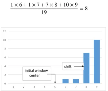
at a random bin as the center of the window. Then, the center of the window is shifted in the direction of the centroid of all the points that fall within the window, namely towards the higher density region. This is repeated until the window converges at a mode of the histogram. This mode represents a cluster and all bins that converge to the same mode are assigned to the same cluster. The process is repeated until all bins are associated with one of the computed modes/clusters. The details of the above iterative mode search are shown below.

1. Place a window center at a randomly selected binbi.

cw =bi (3.3)

2. Repeat till convergence:

2.1. compute the weighted centrorid which will be the new center of the window

cw= P

bj≤cw+w and bj≥cw−wbig(bi)

P

bj≤cw+w and bj≥cw−wg(bj)

(3.4)

The shift procedure is illustrated in Figure 3.1 for a one-dimensional feature vector, e.g., intensity. In the figure, a nine bins window is shown, centered on bin five. The first five bins have count zero, while the other four bins have nonzero values giving nineteen in total. The new mean is computed as

1×6+1×7+7×8+10×9

19 = 8 (3.5)

Figure 3.1: Example of mean shift for 1D histogram

Naturally the mean shift approach can be applied to multidimensional vectors. In our work, feature vectors for each pixel are comprised from color and location.

Finding the mode associated with each data point helps to smooth the image while preserv-ing discontinuities. Two points that are far from each other in the feature space would not fall in the same window and therefore will likely converge to two different clusters. Hence, pixels on either side of a strong discontinuity will not attract each other. By controlling the size of the window in color and space with bandwidth (hs,hc), we can determine the resolution of the

mode detection. If the window size is not appropriate the results can be noisy. In this case it is possible to run a filtering post-processing which will remove/merge small neighboring clusters. In [9], a simple linkage clustering is used for grouping modes which are less than one window size apart and their corresponding data points are merged. This simple procedure ef-fectively converts the noisy results into smooth. The authors in [8] suggest to build a region adjacency graph to hierarchically cluster the modes. But color information may not be suffi -cient, since there might be color overlap between the object and the background. They also proposed to combine edge information with color information to get better clustering results.

Figure 3.2 shows examples of mean shift segmentations for different values of the window bandwidth parameter hc in the color space. Small changes in this parameter can make large

differences in the segmentation results. Figure 3.2(a) shows the original image. When the color bandwidth is small, we get an over-segmented image in Figure 3.2(b). As we increase the value of the color bandwidth, we get reasonable segmentation results with clear objects boundary in Figure 3.2(f). Figure 3.2(g) shows a segmentation result for a large color bandwidth.

(a) (b) (c) (d)

(e) (f) (g)

Figure 3.2: Example of mean shift segmentation with different color features: (a) Origianl image, (b)-(g) mean shift segmentation using scale bandwidth 7 and color bandwidths 3, 7, 11, 15, 19 and 23 respectively. [28]

3.3. EfficientGraph-basedImageSegmentation 21

3.3

E

ffi

cient Graph-based Image Segmentation

Another method to cluster image pixels in the feature space is efficient graph-based image segmentation as described in [11]. Different from mean shift, this method does not need to perform a filtering step first. It directly works on the data points in feature space and uses a adaptive threshold instead of a constant threshold on single linkage clustering. In this section, we first introduce the graph-based representation of the image, then describe the metric for comparing the dissimilarity inside one region and between regions, and give a brief overview of the complete algorithm at last.

3.3.1

Graph-based segmentation

LetG =(V,E) represent an undirected graph, in whichVis the set of vertices andEis the set of edges. It is the set of verticesVthat needs to be segmented in image segmentation. To measure the dissimilarity between neighboring verticesvi andvj, we use an edge between them with a

corresponding weightw(vi,vj). This dissimilarity between the vertices can be simply measured

by the difference in intensity. Or even more complex, it can be based on color, depth, motion, location or any other local attributes. In [11], an edge weight is based on the color information in the RGB space. Then, the goal of this method is to partition the vertices into two sets such the variance within each set is low compared to the boundary between the sets. The principle of such a partition is that the data points which belong to the same parts are similar and yet data points which belong to different parts are dissimilar. The edge weights give a measurement of dissimilarity between two vertices as we described above, so that edges between vertices belonging to the same region will have low weights whereas edges between vertices belonging to different regions will have high weights.

3.3.2

Pairwise region comparison metric

Using a constant threshold as a criterion for merging clustering does not consider the variability between different regions. This may cause some problems. For example, neighboring regions with low contrast between them may be merged together, whereas neighboring regions with high internal variability may be separated into several components. To avoid this, a metric which has an adaptive threshold taking into account the variability of the region is used. The metric has two dissimilarity components. One is to measure the dissimilarity between two neighboring regions by comparing the data points along their boundary. The other is to measure the dissimilarity of the data points within each region. Internal difference is defined as follows:

Int(C)= max

e∈MST(C,E)w(e) (3.6)

The difference between two different regions is measured as the minimum edge weight connecting these two parts. External difference is defined as follows:

Diff(Ci,Cj)= min vi∈Ci,vj∈Cj,(vi,vj)∈E

w(vi,vj) (3.7)

If there is no edge betweenCiandCj, it means that these two regions are not neighbors, so that

Diff(Ci,Cj) = ∞. And then if the external difference between the two regions is less than the

internal difference inside either of the region plus a variable threshold term, the two regions are allowed to be merged. We define the merged difference as follows:

MInt(Ci,Cj)= min(Int(Ci)+τ(Ci),Int(Cj)+τ(Cj)) (3.8)

More specifically, we compare Equation 3.7 with the formula 3.8. If Equation 3.7 is less than the Equation 3.8, the regions are merged. Therefore, the regions are not combined if there is a strong evidence of a boundary between them. A strong evidence of a boundary is required for small regions and vice versa, so the threshold function is written as follows:

τ(C)= k/|C| (3.9)

The above threshold function implies that a largerk produces larger regions and yet smaller kproduces smaller regions. Instead of constant threshold in traditional linkage clustering, the key to success of this algorithm is this data-dependent thresholding. It is also possible to define

τ(C) based on prior information to favor some desired shape. Using adaptive dissimilarity metric above is robust to outliers, but makes the partition problem NP-hard [11].

3.3.3

Algorithm

Below we describe the algorithm in detail. First, the graphG = (V,E) is formed withmedges andnvertices. Each vertex is a pixel. The final segmentation will beS = (S1, ..,Sr) whereSi

is a cluster of data points. The pseudo-code for the efficient graph-based image segmentation is illustrated in Algorithm 1.

Algorithm 1Efficient Graph-based Image segmentation

Input: G =(V,E) andw(vi,vj)∀vi,vj ∈V andvi , vj

1: SortE intoE0 = (e1, ...,em) in non-decreasing order

2: start with a segmentationS0 _{where each vertexv}

iis in a component by itself

3: Leteq =(vi,vj). Repeat step 3 forq=1, ...,mto findSq givenSq−1

4: if viandvjare in disjoint components ofSq−1then

5: ifw(eq) is less than MInt(Ci,Cj) wherevi ∈Ci andvj ∈Cj then

6: MergeCiandCj

7: end if

8: end if

Output: Sm

3.3. EfficientGraph-basedImageSegmentation 23

Figure 3.3: A synthetic image (320× 240 grey image), and the segmentation results (σ = 0.8,k= 300) [11].

Figure 3.4: A street scene (320×240 color image), and the segmentation results (σ=0.8,k = 300) [11].

Gaussian filter is often used first to remove artifacts and smooth the image before segmentation. Some segmentation results implemented in [11] are shown here.

Chapter 4

Energy Minimization using Graph Cuts

For each frame in a video, we formulate background subtraction as a binary labeling problem where the goal is to assign each image pixel either a ”foreground” (or object) or a ”background” label. We solve this binary pixel labeling problem in a principled energy minimization frame-work. The advantage of using energy minimization framework is that we can encode useful problem constraints, such as the requirement that the foreground and background regions are spatially coherent. After the energy function is formulated, we can use optimization algorithm to do energy minimization. The advantage of our energy is that it can be efficiently and globally optimized with a single graph cut [5].

In this chapter, we introduce the labeling problems and a common form of energy function first. Then we give an overview of the energy minimization method based on graph cuts and finally describle a new color separation energy term used in the energy function, which can be globally minimized with a single graph cut [31].

4.1

Labeling Problem and Energy Minimization Framework

Many problems in computer vision can be formulated as labeling problems. In a labeling problem, one has a set of sites and a set of labels. The set of sites is usually all the image pixels. The set of labels are application dependent. The goal is to to assign each site a label from the label set.

To describe the labeling problem more formally, let P be the set of sites and L be the set of labels. The set of sites could be image pixels, medical volume voxels, and any other image entity to which we wish to assign a label. In this thesis, we will assume that sites are image pixels. A labeling problem now can be described as assigning a label fp to each pixel

p∈ P. The collection of all pixel label assignments will be denoted by f. The labels can have a semantic meaning, such as ”house”, ”person”, ”vehicle”, or geometric meaning such as ”left oriented surface”, ”right oriented surface”, etc. Many other meanings of labels are possible. In this work, we need only two labels, the ”foreground” and the ”background”. We identify the foreground with label 1 and the background with label 0. Thus our label set is binary and is equal to{0,1}.

If the label set for all pixels is the same, i.e. L, then the labeling f belongs to the set

L= L × L ×...× L (4.1)

Thus the total number of different possible labelings f is exponentially large, even in the case when the label setL is binary. Any naive method for optimization, such as exhaustive search, is not feasible.

To solve the labeling problem in the energy minimization framework, we design an energy function E(f). The energy function E(f) measures whether labeling f is a good solution to the problem or not. That is E(f) should output a small value if labeling f is considered good labeling, andE(f) should output a large number if f is not satisfactory. A number of criteria can be used by the energy function to judge whether f is a good labeling or not. Most commonly E(f) consists of two terms, the data and the smoothness, both evaluating different aspects of how good a labeling f is. The typical form of energyE(f) is as follows:

E(f)= Edata(f)+λ·Esmooth(f) (4.2)

In Equation 4.2, the Edata is called data term, because this term penalizes labels

inconsis-tency with the observed data according to some data model known a priori, or estimated from the user marked regions, or learned from a dataset with ground truth. Esmooth term is called

smoothness term, it measures how smooth or regular the boundaries between regions with dif-ferent labels are. A typical model used in the smoothness term penalizes any two adjacent pixels that have different labels. If the label set has many labels, then typically a larger label difference is penalized more. However in our case, there are only two labels. Thus either two nearby pixels have exactly the same label, in which case there is no penalty, or they have diff er-ent labels, in which case there is a penalty. The weightλ >0 measures the relative importance of smoothness versus the data terms. Ifλis small, then the smoothness term is not so important and we are looking for a labeling which fits the data terms closely. Ifλis large, then the data term is less important and a labeling with less discontinuities between the labels of nearby pix-els is preferred. Thus the choice ofλis very important. It is chosen either through a parameter learning technique, or estimated experimentally on validation data through grid search.

The typical form for data term is as follows:

Edata(f)= X

p∈P

Dp(fp) (4.3)

where Dp measures the penalty for assigning pixel p to the label fp, according to the data

model. The data model can be based on image intensity, color and etc. For example, let us consider a simple case. Suppose we know a priori that the background should have intensity 20 or lower and the object should have intensity 220 or higher. Then a good choice for the data term isDp(0)=max(Ip−20,0) andDp(1)= max(220−Ip,0).

The smoothness term is typically written as,

Esmoothness(f)= X

pq∈N

Vpq(fp, fq) (4.4)

4.2. Optimization withGraphCuts 27

Figure 4.1: Illustration of 4 and 8 neighborhood systems in images

The smoothness term penalizes the discontinuties between neighboring pixels. The more similarity the two neighboring pixels have, the larger is the penalty if they are assigned different labels. Parameterλis used to adjust the relative weight of the smoothness term versus the data term.

4.2

Optimization with Graph Cuts

A graph cut is a popular energy optimization algorithm in computer vision. It has been suc-cessfully used in many applications [3]. In this work, the optimization algorithm is also based on computing a graph cut of minimum cost [5]. In this section, we will briefly describe the graph cut optimization algorithm which is based on the max-flow/min-cut theorem. Then we discuss how a graph cut is applied to the binary labeling problem.

Let G = (V,E) be a connected weighted graph with vertices V and edges E. The set of vertices contains two special vertices, called the source sand the sinkt. Figure 4.2 shows an example of a graph with source and sink vertices. An s−tcutC = (S,T) segments vertices V into two setsSand T, such that s ∈ S, t ∈ T and V = S ∪ T. More specifically, a cutC is a subset of edgesE, such that when edges inC are removed from the graphG, verticesV is partitioned into two disjoint setsSandT. The cost of the cutCis computed as follows,

|C|= X

e∈C

we (4.5)

wherewe is the weight of edgee ∈ E. Figure 4.3 shows an example of s−t graph cut with

terminals s and t. It is shown for a 4-connected neighborhood. The thickness of the edge is directly proportional to the edge weight. The aim of the minimum cut problem is to find a cut with the minimum cost among all possible cuts in the graphG. The green dashed curve shown in Figure 4.3 illustrates a minimum cut, that is the cut with the lowest cost.

to the sink t. In [16], they describe each edge of the graph as a pipe with a capacity that is equal to its weight. Thus the flow that one can push through an edge cannot be larger than the capacity of that edge. Then, maximum flow is explained as the maximum ”amount of water” that can be sent from the source to the sink [6]. A maximum flow from source to tink saturates a set of edges in the graph. An edge is saturated if the flow through that edge is equal to the weight (or capacity) of that edge. These saturated edges divides the nodes into two disjoint parts corresponding to a minimum cut [16]. Thus, the minimum cut problem is equivalent to the maximum flow problem.

More specifically, the flow from one node to another is denoted as a function f : V×V →

R. The value of the flow for the graphG=(V,E) is defined as follows:

|f|= X

v∈V

f(s,v) (4.6)

where f(s,v) means the flow sent out of the source s tov. If the edge (u,v) is non saturated, we call the additional amount of flow as residual capacitycf(u,v).

cf(u,v)=c(u,v)− f(u,v) (4.7)

wherec(u,v) denotes the capacity of the edge, f(u,v) denotes the flow sent fromutov. Consider a path p = (s,v1,v2, ...,t) with no repeated vertices from s to t, we define the residual capacity of the path as below:

cf(p)=min{cf(u,v)|(u,v)∈ p} (4.8)

If we iteratively send flows from the source to the sink till no more flow can pass through the edges, each path reach the lowest residual capacity with a saturated edge, then we have sent the maximum flow from the source to sink.

Figure 4.2: An example of a graph with source and sink terminals. [Image credit: Yuri Boykov]

Then, the process of max-flow/min-cut algorithm is described as following steps. Figure 4.4 also gives an intuitive description.

1. First, find a flow path f from sto t along non saturated edges, which means that the capacity of the flow f is smaller than all edges weight along the path.

2. Increase flow f along this path until some edge saturates. The edge become saturated when the capacity of the flow f is equal its edge weight.

4.2. Optimization withGraphCuts 29

Figure 4.3: An example of as−tcut on a graph. [Image credit: Yuri Boykov]

(a) (b)

(c)

4. All the saturated edges found in the former steps form the minimum cut.

The algorithm introduced before is one of the popular algorithms to compute the maximum flow of a given graph. It is the basic maximum flow algorithm proposed by Ford-Fulkerson. Edmonds-Karp presented another method to compute the maximum flow, which is an improve-ment of Ford-Fulkerson’s algorithm in terms of computational efficiency. More details are in [10].

Generally, the optimization of the energy Equation 4.2 is an NP-hard problem, even when dealing with the binary energy. But in some special cases, a global optimum of the energy function can be found by finding a minimum cut on a certain graph. In particular, if a binary energy function is submodular, then it can be minimized exactly with finding a minimum cut on a certain graph. In this thesis, we choose to use the max-flow/min-cut algorithm developed by Boykov and Kolmogorov [6] as it is particularly efficient in practice for the graphs that arise in computer vision problems.

For binary energies, Kolmogorov [20] showed that the energy function is submodular if

Vpq(0,0)+Vpq(1,1)≤Vpq(0,1)+Vpq(1,0) (4.9)

whereVpqis the pairwise smoothness term in the energy function,

E(f)= X

p∈P

Dp(fp)+λ X

pq∈N

Vpq(fp, fq) (4.10)

Consider a simple 3 by 3 image as an example for binary energy optimization. As shown in Figure 4.5, we first need to construct a graph G = (V,E) based on the original image. The pixels in the image correspond to graph verticesVand the neighboring pixels are connected by graph edgesE. There are two special terminal nodes source sand sinkt, corresponding to the two different labels in binary optimization problem. Each pixel node in the constructed graph is connected to the terminal nodes source sand sinkt by an edge usually calledt−link. The data termDp(fp) in the energy function is used for the weight oft−link, and it corresponds to

the penalty of assigning label fpto pixel p∈ P. In this work,Dp(fp) is computed based on the

difference between background model and the current image, where fp ∈0,1.

The links between neighboring pixel nodes are usually called n−links. The smoothness term is used for the weight ofn−link, which penalizes the discontinuity between the neigh-boring pixel nodes. More specifically, the more similar the two neighneigh-boring pixel nodes pand qare, the higher the Vpq is to prevent assigning them to different labels. The measurement of

the weight between neighboring pixel nodes is performed in different ways. For example, in grayscale images the similarity can be computed on local gradient of intensity.

4.2. Optimization withGraphCuts 31