Scholarship@Western
Scholarship@Western
Electronic Thesis and Dissertation Repository
5-3-2017 12:00 AM
Developing and Testing a Model of Site Amplification for Southern
Developing and Testing a Model of Site Amplification for Southern
Ontario
Ontario
Sebastian Braganza Western University
Supervisor Dr. Gail Atkinson
The University of Western Ontario Graduate Program in Geophysics
A thesis submitted in partial fulfillment of the requirements for the degree in Master of Science © Sebastian Braganza 2017
Follow this and additional works at: https://ir.lib.uwo.ca/etd
Part of the Geophysics and Seismology Commons
Recommended Citation Recommended Citation
Braganza, Sebastian, "Developing and Testing a Model of Site Amplification for Southern Ontario" (2017). Electronic Thesis and Dissertation Repository. 4544.
https://ir.lib.uwo.ca/etd/4544
This Dissertation/Thesis is brought to you for free and open access by Scholarship@Western. It has been accepted for inclusion in Electronic Thesis and Dissertation Repository by an authorized administrator of
ii
Commonly-applied methods to estimate ground-motion amplification for earthquake
hazard applications in southern Ontario are highly generalized. Site amplification effects
have typically been estimated by a parameter that is not well-known in the region, the
time-averaged shear-wave velocity in the top 30 metres of soil; VS30. Moreover, VS30 is not well
correlated with site amplification in this region. This study develops a model that can better
estimate ground motions and shaking intensities in southern Ontario based on
readily-available information. The model is based on a site’s peak response frequency (fpeak), which
can be estimated from depth-to-bedrock. This fpeak-based model estimates ground motions
differently compared to a VS30-based model, as given by the National Building Code of
Canada (NBCC). Field surveys show that the estimate of fpeak is stable over a distance of 1
km. The developed model can be used to estimate site response for building code and
ShakeMap applications.
Keywords
Earthquakes, Ground motion, Site amplification, Peak frequency of response (fpeak),
iii
Co-Authorship Statement
This thesis is prepared in integrated-article format and includes the following
manuscripts written by Sebastian Braganza and the co-authors. Sebastian is the first author
on studies of site amplification in southern Ontario. Sebastian performed the analyses
described in this thesis and authored these reports with assistance from the co-authors.
1) Braganza, S., Atkinson, G.M., Ghofrani, H., Hassani, B., Chouinard, L., Rosset, P.,
Motazedian, D., Hunter, J. (2016). Modeling Site Amplification in Eastern Canada on a
Regional Scale, manuscript published in Seismological Research Letters.
2) Braganza, S., Atkinson, G.M. (2017). A Model for Estimating Amplification Effects on
Seismic Hazards and Scenario Ground Motions in Southern Ontario, manuscript accepted for
publication in the Canadian Journal of Civil Engineering.
3) Braganza, S., Atkinson, G.M., Molnar, S. (2017). Assessment of the Spatial Variability of
Site Response in Southern Ontario, manuscript submitted to Seismological Research Letters.
The thesis and composed articles were completed under the supervision of Dr. Gail
iv
Acknowledgments
First and foremost, I would like to express my utmost gratitude to my supervisor, Dr.
Gail Atkinson, for providing me with the opportunity to work in the engineering seismology
group over the past few years. Under her guidance, I was able to grow as a geoscientist and
successfully complete the three papers related to my thesis. The skills that I learned and
developed as her student are skills that I will undoubtedly use for the rest of my life.
I would also like to thank everyone in the engineering seismology group at Western,
especially Dr. Karen Assatourians, Dr. Hadi Ghofrani, Dr. Behzad Hassani and Dr. Sheri
Molnar. Their help, teachings and suggestions greatly improved the quality of this research.
Last, but not least, I would like to thank my parents. Their love, support and
encouragement have helped me to persevere and are what have made all of my academic
v
Table of Contents
Abstract ……….…….……….……….. ii
Co-Authorship Statement ..……….………….……….. iii
Acknowledgments ………..……….……….……….………... iv
Table of Contents ….……..……….……….……... v
List of Tables ………..……….…….………... viii
List of Figures ………..………..………... ix
List of Appendices ………..……….…….………... xiv
List of Abbreviations ………..……….………….……….……….. xv
Chapter 1 ………..……….……..……….………... 1
1 Introduction …….………..………..……….………..…………... 1
1.1 Motivation for this Research ...…...……….………...……..…………... 1
1.2 Seismicity in Southern Ontario ...………….………...…..…………... 2
1.3 Review of Studies on Site Response Parameters …....………..…………... 4
1.4 Organization of Work ……….………..…………... 6
References …..……….…….………..…………... 7
Chapter 2 ………..………..………….…….……….. 9
2 Modeling Site Amplification in Eastern Canada on a Regional Scale ……..…………... 9
2.1 Introduction………...……….……...……..….………... 9
2.2 Database Information and the Computation and Classification of H/V Curves.... 11
2.3 H/V Characteristics and Correlation between Peak Frequency and Depth to Bedrock ... 14
vi
2.6 Comparisons with a Typical Site Response Model Used in California...28
2.7 Summary and Conclusion ...30
References...31
Chapter 3 ………..………..………….…….………...….. 34
3 A Model for Estimating Amplification Effects on Seismic Hazards and Scenario Ground Motions in Southern Ontario ……….…....……….………... 34
3.1 Introduction………...……..……….…...……..….………... 34
3.2 Derivation of the fpeak-based Amplification Model …………...…..…..….………... 36
3.3 Methods used to Estimate Ground Motion and Intensity ………...…...………... 39
3.3.1 Motions for a Reference Site Condition ………...…...…..….………... 39
3.3.2 Calculation of Site Amplifications Relative to the Reference Site Condition ………...…...…..………….……….………... 42
3.3.3 Conversion of Ground Motion to Intensity ………...…...….………... 44
3.4 Ground Motions and Intensity for the City of Ottawa …….…...…...………... 44
3.5 Felt Intensity Comparisons for Downtown Ottawa ………...………...………... 47
3.6 Ground Motion and Intensity Maps for Southern Ontario ………...…...…...…... 50
3.7 Summary and Conclusions ………...………...………... 54
References...55
Chapter 4 ………..………..………….………...….. 59
4 Assessment of the Spatial Variability of Site Response in Southern Ontario ..……….. 59
4.1 Introduction………...……..………...……..….………... 59
4.2 Microtremor Technique Background ………...……..….………... 61
4.3 Survey Analysis and Methodology……….………...……..….………... 62
vii
References...75
Chapter 5 ………..………..………….………...….. 77
5 Discussion, Conclusions and Future Work..………..………. 77
5.1 Discussion ………...………...………... 77
5.2 Summary and Conclusions ………...………...………... 79
5.3 Future Work ………...……….………...………...80
References...80
Appendices ………..………..………….………...….. 82
viii
List of Tables
Table 3-1: Normalized 2015 NBCC site factors (class A reference) corresponding to
ShakeMap parameters ... 43
Table 4-1: The fpeak values from all (H/V)EQ and (H/V)MT at the 10 stations. The average
difference between log(fpeakEQ/fpeakMT) is computed as the average of all absolute value
ix
List of Figures
Figure 1-1: Horizontal (east-west) acceleration time histories from two strong motion stations
in Mexico City during the M8.0 Michoacan earthquake. Station UNAM was situated on
basaltic rock, while SCT was located on soft soil (from Kramer, 1996) ………. 2
Figure 1-2: The earthquake size and distribution in southern Ontario. Earthquakes are
presented as Nuttli magnitudes (MN). The cluster of events in the northeast corner of the map
originate from the Western Quebec Seismic Zone (from Assatourians et al, 2013) ………... 3
Figure 1-3: Examples of H/V spectra from Class I (left) and Class II (right) regions. H/V
spectra in Class I regions are typically more distinct and have greater peak amplitudes. Note
that the H/V is in base 10 log units. A standard Gaussian curve, derived from empirical data
from Japan, is superimposed on both plots (from Ghofrani and Atkinson, 2014) …………... 5
Figure 2-1: Sediment thickness (D) across southern Ontario and the locations of seismograph
stations used in this study ……….…………. 13
Figure 2-2: Average velocity-depth profiles for the study region. The dashed lines represent
profiles for the cities of Montreal and Ottawa while the solid black line is the profile
proposed for the entire region. Note that these profiles are derived primarily from sand/clay
sites ………..……….…………. 16
Figure 2-3: Site peak frequencies plotted as a function of depth-to-bedrock. Three fpeak =
Vsav/(4D) relations, based on three average velocity profiles (discussed in text), are
superimposed …………...……….…………. 17
Figure 2-4: H/V spectra from 15 seismograph stations on till, plotted by f/fpeak with the
weighted average H/V curve and till amplification function. The spectra have an average
Apeak of 3.0 .…………...………..………..…………. 19
Figure 2-5: H/V spectra from 7 seismograph stations on sand/clay, plotted by f/fpeak with
weighted average H/V curve and sand/clay amplification function. The spectra have an
x
f/fpeak, and the soft organic sediment amplification function. The H/V spectrum has an Apeak
of 9.5 ………...………..……….…………. 21
Figure 2-7: H/V spectra from 15 seismograph stations on bedrock with the weighted average
H/V curve and bedrock amplification function. The spectra rise gently with increasing
frequency …...………..………..…………. 23
Figure 2-8: Comparison of site amplification functions for different surficial geology types.
Till, sand/clay and very soft sediment/fill are plotted with respect to normalized
frequency………...………..………..………….. 25
Figure 2-9: Suggested amplification functions for generic sites with poorly-known fpeak,
normalized by fpeak …...………..……….……….…….……. 27
Figure 2-10: The three proposed generic sediment amplification functions for eastern Canada
and the corresponding functions for California (Seyhan and Stewart, 2012) assuming nominal
values of VS30 of 1000 m/s, 300 m/s and 150 m/s for till, sand/clay and soft soil, respectively.
Light shades refer to very soft sediment/fill; intermediate to sand/clay; dark to till ...….…. 29
Figure 3-1: The Braganza et al. (2016) linear amplification model for southern Ontario,
showing amplification factors for 1 Hz (a) and 10 Hz (b) ground motions. Soil nonlinearity
may reduce these factors for strong levels of shaking ...………...…. 36
Figure 3-2: Linear amplification functions for sites with unknown fpeak, normalized by
fpeak ……….………. 38
Figure 3-3: Attenuation curves for the Val-des-Bois and scenario M6.0 earthquakes for PSA
at 1 and 10 Hz (a) and expected response spectra for the city of Ottawa for the Val-des-Bois
and 2% in 50 year motions (b). The response spectrum for the M6.0 scenario event at a
distance of 20 km is also shown. All curves are for a class A (hard rock) reference ……… 41
Figure 3-4: Estimated 1 Hz (a) and 10 Hz (b) log(PSA) for Ottawa for the M5.0 Val-des-Bois
xi
The locations of Orléans (discussed in text) and downtown Ottawa are indicated ……...… 46
Figure 3-5: Estimated 1 Hz (a) and 10 Hz (b) horizontal log(PSA) for Ottawa from its 2% in
50 year probability ground motions, using the fpeak-based amplification model ………...… 47
Figure 3-6: Estimated NEHRP site class and depth-to-bedrock from microzonation
information (Motazedian et al., 2011) for downtown Ottawa and Orléans. Pal and Atkinson
(2012) examined reported felt intensity for the M5.0 Val-des-Bois earthquake for this area ………. 48
Figure 3-7: Estimated MMI for the M5.0 Val-des-Bois earthquake, along with differences
between observed and predicted intensities ………..………. 49
Figure 3-8: Estimated 1 Hz (a) and 10 Hz (b) horizontal log(PSA) for southern Ontario for
the M5.0 Val-des-Bois earthquake, using the fpeak-based amplification model ………. 51
Figure 3-9: Estimated 1 Hz (a) and 10 Hz (b) horizontal log(PSA) for a subregion of southern
Ontario for a scenario M6.0 earthquake, using the fpeak-based amplification model. The
estimated log(PSA) differences computed from the NBCC minus the fpeak-based
amplification models are shown for 1 Hz (c) and 10 Hz (d) motions ………...………. 52
Figure 3-10: Estimated intensity map of southern Ontario for the M5.0 Val-des-Bois
earthquake using the fpeak-based model. Observed intensities for six cities are superimposed
for comparison ………..………. 53
Figure 3-11: Estimated intensity map of the Niagara Peninsula region of southern Ontario for
a scenario M6.0 earthquake using the fpeak-based model (a). The intensity differences
computed from the NBCC and fpeak-based models are also shown (b) ...……..………. 54
Figure 4-1: Site amplification functions from Braganza et al. (2016) for sites in southern
Ontario (fpeak to be determined from regionally mapped depth-to-bedrock estimates). The
functions for sediment (till, sand/clay and very soft sediment) are normalized to a
dimensionless f/fpeak value of 1, whereas the function for bedrock is a function of frequency
xii
stations. Stations are on sediments of varying type and thickness. Note that station TORO is
located on a small, man-made peninsula south of the city of Toronto ...……..………. 62
Figure 4-3: The MoHo s.r.l. Tromino® used to perform ambient noise (microtremor) surveys
in this study………. 63
Figure 4-4: Examples of poor and good ambient noise recordings near station ACTO.
Individual component spectra for the 0 m survey do not exhibit a distinct “eye-shape”
divergence between the vertical and horizontal components, resulting in a (H/V)MT that is
without a clear peak. By contrast, the 40 m survey shows a divergence between components
at ~8-15 Hz, resulting in a clear spectral peak at ~13 Hz ...………..………. 65
Figure 4-5: Station TORO's (H/V)EQ (heavy line) and the six (H/V)MT surveys, at distances
up to 1 km. All surveys show a consistent fpeak of 1.0 Hz ..……..………. 66
Figure 4-6: Station PKRO's (H/V)EQ (heavy line) and the six (H/V)MT surveys, at distances
up to 1 km. An fpeak of 1.6 Hz is seen at distances < 80 m, which decreases to 1.3 Hz (0.1 log
units) from 160 m to 1 km ………..……..………. 66
Figure 4-7: Station ELFO's (H/V)EQ exhibits a fairly broad peak with fpeak at 2.5 Hz, followed
by a secondary smaller peak at 4.0 Hz. This is reflected in the (H/V)MT, which show either
double peaks or broad spectra at all survey distances ………....……..………. 68
Figure 4-8: DRWO's (H/V)EQ has an fpeak at 4.0 Hz, but the spectrum is similar in H/V ratio
between 3.3 Hz to 5.0 Hz. The (H/V)MT show fpeak variations in this entire range, with a
higher fpeak of 5.0 Hz for the 500 and 1000 m surveys ………...……..………. 69
Figure 4-9: (H/V)MT at station BRCO show noise contamination below ~1 Hz, but the spectra
still show a general agreement in fpeak (2.0 Hz) with that from the (H/V)EQ ………. 70
Figure 4-10: H/V ratios at station ACTO. The 40 and 80 m surveys exhibit a log(fpeak) that is
within 0.1 units of the fpeak from (H/V)EQ (10.2 Hz), while the 160 m survey shows greater
xiii
ambient noise H/V ratios at 1 km distance from each station. fpeak is shown to be in
agreement to within 0.13 log units, on average ………. 73
Figure 5-1: Map of the study area (Greater Toronto Area) from Mihaylov (2011), in addition
to interpolated values of fpeak, determined from ambient noise surveys at 187 test sites.
Nearby seismograph stations (ACTO, TORO and PKRO) and their station fpeak values are
superimposed ………. 77
Figure 5-2: Measured fpeak, as determined from a microzonation study in the Greater Toronto
Area (Mihaylov, 2011) versus estimated fpeak, as determined using equations (2.1) and (2.4)
xiv
List of Appendices
Appendix A: The log horizontal-to-vertical (H/V) ratios of the 38 seismograph stations in
eastern Canada ………..………. 82
Appendix B: The standard deviations of the log horizontal-to-vertical (H/V) ratios of the 38
seismograph stations in eastern Canada ………….………...………. 84
Appendix C: The 38 stations’ site and horizontal-to-vertical (H/V) spectral characteristics ………. 86
Appendix D: Tromino deployment and processing methods, and horizontal-to-vertical (H/V)
xv
List of Abbreviations
ENA Eastern North America
OGS Ontario Geological Survey
GMICE Ground-motion-to-intensity conversion equation
NEHRP National Earthquake Hazards Reduction Program
NBCC National Building Code of Canada
MMI Modified Mercalli Intensity
GMPE Ground-motion prediction equation
PSA Pseudo-spectral acceleration
PGV Peak ground velocity
PGA Peak ground acceleration
PGAref Expected PGA for a reference site class C
PGAr PGA as estimated by GMPE from Boore et al. (2014)
UHS Uniform hazard spectrum
SEED Standard for the Exchange of Earthquake Data
H/V Horizontal-to-vertical spectral ratio
(H/V)EQ Earthquake horizontal-to-vertical spectral ratio
(H/V)MT Microtremor horizontal-to-vertical spectral ratio
VS Shear-wave velocity
xvi
Fnl Linear component of site amplification
Flin Nonlinear component of site amplification
Fs Total site amplification
fpeak Peak frequency of response
Apeak Peak amplitude of response
A Amplification factor
g Acceleration due to gravity (9.81 m/s2)
D Depth-to-bedrock
T Fundamental site period
n Number of felt intensity reports
M Moment magnitude
Chapter 1
1
Introduction
1.1
Motivation for this Research
The amplification of seismic waves in soft, surficial sediment layers is referred to
as site amplification or site response. This physical phenomenon has been observed
throughout the world and for many different earthquakes. Its occurrence is due to a
simple principle related to the conservation of energy: as shear waves from deeper layers
travel to the surface of the earth, they will enter layers that are typically softer and less
dense, and as a result, the shear-wave velocity will decrease; thus, the amplitude of the
waves will increase. Since shear waves refract toward the vertical as they enter softer
layers of sediment and since their direction of particle motion is perpendicular to the
direction of propagation, the amplification of these waves occurs primarily in the
horizontal direction. It is this horizontal shaking that is associated with felt shaking and
increased damage that is observed during earthquakes (e.g., Trifunac and Todorovska,
1997).
An excellent illustration of site amplification is the 1985 Michoacan (Mexico
City) earthquake. The moment magnitude (M) 8.0 earthquake resulted in only moderate
damage near the epicenter where rock is prominent, but extensive structural damage was
observed ~350 km away in Mexico City, which is dominated by soft clay sediments
(Kramer, 1996). Even within Mexico City, strong-motion instruments recorded vastly
different horizontal ground accelerations, depending on whether the instrument was on
rock or soft clay. Figure 1-1 shows an example of contrasting horizontal acceleration
records from two different sites for this earthquake; strong-motion station UNAM was
situated on basaltic rock, while station SCT was located on soft soil. The record from
Figure 1-1: Horizontal (east-west) acceleration time histories from two strong
motion stations in Mexico City during the M8.0 Michoacan earthquake. Station
UNAM was situated on basaltic rock, while SCT was located on soft soil (from
Kramer, 1996).
While the site amplification example of Mexico City is a fairly extreme one, the
phenomenon will exist to some extent for any region that is home to varying surficial soil
types. In this study, the focus is on predicting site response in Canada’s most
densely-populated region: southern Ontario.
1.2
Seismicity in Southern Ontario
Southern Ontario is a fairly stable seismic region when compared to active
regions such as California or Japan. The region does not frequently experience damaging
earthquakes, as it is located in the middle of the North American Plate. However,
small-to-moderate earthquakes of M3 to 5 (with M ≈ 4.5 being the damage threshold) occur
frequently throughout the region, with larger events occurring less frequently. Many of
these earthquakes originate in the Western Quebec Seismic Zone, which extends more
than 500 km from the Timiskaming region of Quebec, through the Ottawa-Montreal
corridor, to the Adirondack Highlands of New York (Ma and Eaton, 2007; Basham et al.,
1979). The Southern Great Lakes Seismic Zone is also host to earthquakes of M3 to 5,
although they occur infrequently here. It has been hypothesized that earthquakes
occurring in the region below Lake Ontario can be attributed to fluids, which alter the
the distribution of earthquakes in southern Ontario during the time period from 1991 to
2013 (Assatourians et al., 2013).
Figure 1-2: Seismicity in southern Ontario (1991 to 2013). Earthquake symbol sizes
are scaled by their magnitudes (based on the Nuttli magnitude scale, MN). The
cluster of events in the northeast corner of the map originate from the Western
Quebec Seismic Zone (from Assatourians et al., 2013).
A few notable twenty-first century earthquakes to be felt in the region are the
2002 M5.0 Au Sable Forks, New York (Atkinson and Sonley, 2003), 2010 M5.0
Val-des-Bois, Quebec (Atkinson and Assatourians, 2010), and 2013 M4.5 Ladysmith, Quebec
(Atkinson et al., 2014), earthquakes. Thus, even though southern Ontario has relatively
low levels of seismic activity, the region still periodically experiences earthquakes that
considered moderate, despite the relatively-low activity levels, due to the region’s high
population density. Assessments on how seismicity and site amplification impacts the
region are therefore important.
1.3
Review of Studies on Site Response Parameters
Ground-motion prediction equations (GMPEs) are a common way to describe
expected earthquake motions, accounting for average earthquake source, path and site
effects. The site term in the GMPE commonly uses shear-wave velocity in the top 30
metres of soil (VS30) as the descriptive variable. Denser/stiffer soil materials are
associated with higher VS30 values. In many applications, VS30 is estimated based on
correlations with topographic slope (Wald and Allen, 2007). The shortfall with this proxy
method is that it does not work well in regions like southern Ontario that have subdued
topographic relief. However, using site-specific studies to obtain more accurate VS30
values can be an expensive and time-consuming procedure. Moreover, many seismograph
stations in southern Ontario only have inferred or assumed values of VS30, making the
degree of correlation between VS30 and site amplification difficult to assess. Using
alternative approaches to estimate site response in southern Ontario is therefore
appealing.
Alternative methods for estimating site response include the horizontal-to-vertical
(H/V) ratio method, which uses spectral ratios of ground motions to estimate a site’s peak
frequency of response (fpeak), in addition to other parameters, such as a site’s surficial
geology. The fpeak of a site is typically within a narrow frequency bandwidth, within
which the H/V ratio is at a maximum; this is related to the site’s subsurface properties
(e.g., sediment thickness). The benefit of using fpeak as a site response variable is that it is
relatively easy to obtain and it provides information for sites that are deeper than 30 m.
Moreover, characterizing shallow sites (< 30 m) can be problematic when using VS30 if
there is an intrusion of high-velocity bedrock in the top 30 m (e.g., McPherson and Hall,
2013).
A number of recent studies have examined the use of fpeak as a site response
(2012) used site periods from H/V spectral ratios as a means for site classification and
found that the H/V ratio method reduced the standard deviation from GMPEs and better
captured the long and short period resonance from deep and shallow soil sites,
respectively. In Japan, Zhao and Xu (2013) and Ghofrani and Atkinson (2014) similarly
found that fpeak or site period from H/V ratios was a better predictive site variable than
VS30 for longer period (or deeper) sites. Moreover, larger and more distinct peaks in
amplification spectra are expected in regions like Japan where there exists a soft sediment
layer overlying hard bedrock (Class I regions), providing conditions for a strong
impedance contrast (Aki and Richards, 2002; Ghofrani and Atkinson, 2014). This differs
from regions like California (Class II), which are characterized by a gradational soil
profile, resulting in broader amplification spectra, lower spectral peak amplitudes, and
peaks at lower frequencies. Figure 1-3 shows examples of H/V spectra from Class I and
II regions. Since southern Ontario is characterized by a range of soil types overlying very
hard, glaciated bedrock (shear-wave velocity or VS ≈ 2800 m/s; Boore and Joyner, 1997),
it is expected that H/V spectra in the region will resemble that of Class I regions, such as
Japan; thus, the argument for fpeak being a more applicable site response variable than
VS30 likely also applies to southern Ontario.
Figure 1-3: Examples of H/V spectra from Class I (left) and Class II (right) regions.
amplitudes. Note that the H/V is in base 10 log units. A standard Gaussian curve,
derived from empirical data from Japan, is superimposed on both plots (from
Ghofrani and Atkinson, 2014).
1.4
Organization of Work
In chapter 2, we use H/V spectral ratios from earthquake records in southern
Ontario in order to characterize site response in the region. We show that site response
can be modeled using a couple of variables that are readily obtainable: fpeak (determined
from the H/V ratio or sediment depth) and surficial geology or sediment type. These
variables are used to create a preliminary model of site amplification that can be used
with GMPEs for the region, as well as for predicting ground motions or shaking intensity
on a regional scale. Chapter 2 has been published as Modeling Site Amplification in
Eastern Canada on a Regional Scale in Seismological Research Letters.
In chapter 3, the site amplification model based on fpeak is compared to one based
on VS30, as given by the 2015 National Building Code of Canada (NBCC). Earthquakes
and scenario events are used to estimate ground motions and shaking intensities. It is
shown that both models generally predict similar felt intensities but show significant
differences in their predicted amplification of ground motions as a function of frequency.
The results of this chapter support the use of fpeak as a site response variable for
estimating amplification effects in southern Ontario. Chapter 3 has been accepted for
publication as A Model for Estimating Amplification Effects on Seismic Hazards and
Scenario Ground Motions in Southern Ontario in the Canadian Journal of Civil
Engineering.
In chapter 4, we measure the spatial variability of fpeak within 1 km distance of 10
seismograph stations in southern Ontario. Establishing spatial variability of fpeak is useful
for assessment of regional site response and its uncertainty: we can estimate site response
if fpeak is known, and thus it is important to know to what distances the value of fpeak is
spatially stable. We find that, on average, log10(fpeak) as measured by microtremor survey
H/V from earthquake records), for survey sites within 1 km of the station. Chapter 4 has
been submitted for publication as Assessment of the Spatial Variability of Site Response
in Southern Ontario in Seismological Research Letters.
Finally, a summary of all findings is provided in chapter 5, in addition to
suggestions for future work.
References
Aki, K and Richards, P.G. (2002). Quantitative Seismology, 2nd edition.University
Science Books. Sausalito, California. 700.
Assatourians, K., Atkinson, G.M., Dunn, B. and Li, M. (2013). The Southern Ontario
Seismograph Network Activity Report for Ontario Power Generation. Department
of Earth Sciences, The University of Western Ontario. 165.
Atkinson, G.M. and Sonley, E. (2003). Ground Motions from the 2002 Au Sable Forks
M5.0 Earthquake. Seismological Research Letters, 74, no. 3, 399–349.
Atkinson, G.M. and Assatourians, K. (2010). Attenuation and Source Characteristics of
the 23 June 2010 M 5.0 Val-des-Bois, Quebec, Earthquake. Seismological
Research Letters, 81, 849–860.
Atkinson, G.M., Assatourians, K. and Lamontagne, M. (2014). Characteristics of the 17
May 2013 M 4.5 Ladysmith, Quebec, Earthquake. Seismological Research
Letters, 85, no. 3, 755–762.
Basham, D.M., Weichert, D.H., and Berry, M.J. (1979). Regional assessment of seismic
risk in eastern Canada. Bulletin of the Seismological Society of America, 11,
1567–1602.
Boore, D.M., and Joyner, W.B. (1997). Site Amplifications for Generic Rock Sites,
Bulletin of the Seismological Society of America, 87, no. 2, 327–341.
Di Alessandro, C., Bonilla, L.F., Boore, D.M., Rovelli, A. and Scotti, O. (2012).
Predominant-Period Site Classification for Response Spectra Prediction Equations
in Italy. Bulletin of the Seismological Society of America, 102, no. 2, 680–695.
Vertical Response Spectral Ratios of Earthquakes in the NGA-West 2 and
Japanese Databases. Bulletin of Soil Dynamics and Earthquake Engineering, 67,
30–43.
Kramer, S.L. (1996). Geotechnical Earthquake Engineering. Prentice-Hall, Inc. Upper
Saddle River, New Jersey. 653.
Ma, S. and Eaton, D. (2007). Western Quebec seismic zone (Canada): Clustered, mid-
crustal seismicity along a Mesozoic hot spot track. Journal of Geophysical
Research, 17, 16.
McPherson, A. and Hall, L. (2013). Site Classification for Earthquake Hazard and Risk
Assessment in Australia. Bulletin of the Seismological Society of America, 103,
no. 2A, 1085–1102.
Mereu, R.F., Asmis, H.W., Dunn, B., Brunet, J., Eaton, D., Dineva, S. and Yapp, A.
(2002). The Seismicity of the Western Lake Ontario Area: Results from the
Southern Ontario Seismic Network (SOSN), 1992-2001. Seismological Research
Letters, 73, no. 4, 534–551.
Trifunac, M.D. and Todorovska, M.I. (1997). Northridge, California, Earthquake of
1994: density and red-tagged buildings versus peak horizontal velocity and
intensity of shaking. Soil Dynamics and Earthquake Engineering, 16, no. 3, 209–
222.
Wald, D.J. and Allen, T.I. (2007). Topographic Slope as a Proxy for Seismic Site
Conditions and Amplification. Bulletin of the Seismological Society of America,
97, 5, 1379–1395.
Zhao, J.X. and Xu, H. (2013). A Comparison of VS30 and Site Period as Site Effect
Parameters in Response Spectral Ground-Motion Prediction Equations. Bulletin of
Chapter 2
2
Modeling Site Amplification in Eastern Canada on a
Regional Scale
2.1
Introduction
Eastern North America (ENA) has relatively low levels of seismic activity, but
earthquakes nevertheless pose a moderate risk due to densely-populated urban centers
and critical infrastructure. Moreover, sediments in many parts of ENA tend to strongly
amplify ground motions from moderate earthquakes. A good example of this is the
moment magnitude (M) 5.0 Val-des-Bois earthquake, which had a felt area of
approximately 3 million km2 and produced the strongest shaking ever felt in Canada’s
capital city of Ottawa, more than 60 km away (Atkinson and Assatourians, 2010); the
shaking in Ottawa was particularly strong on soil sites (Pal and Atkinson, 2012). The
sediments in ENA are comprised of postglacial sands, clays and tills of variable stiffness
and thickness, which often overlie very hard glaciated bedrock, providing a sharp contrast
in shear wave velocity. This produces strong and highly variable site amplification within
the region. Proper modeling of these amplification effects is critical in the interpretation
of recorded ground motions and the evaluation of hazard. While this study is focused on
the region extending from southern Ontario to Quebec, the results also apply to other
ENA sites which share similar characteristics.
Horizontal-to-vertical (H/V) component spectral ratios of Fourier amplitude
spectra and/or response spectra (e.g., pseudo-spectral acceleration, PSA) are known to be
a measure of site amplification, particularly effective at identifying the predominant site
frequency (e.g., Nakamura, 1989; Lermo and Chávez-Garcia, 1993; Kawase et al., 2011).
Horizontal-component shear-wave motions are amplified in near-surface sediment layers,
whereas amplification on the vertical component is counterbalanced by the ray path
refracting toward the vertical. Thus, the vertical component amplification may be
considered negligible relative to that of the horizontal component, so that H/V ratios are a
development of ground-motion prediction equations (GMPEs), and for mapping the
intensity of ground motion (e.g., ShakeMaps; Wald et al., 1999).
In this study, we use seismograph station and microtremor H/V measurements,
from southern Ontario and Quebec, to develop a regional-scale model of site
amplification suitable for use in applications such as ShakeMap. This model consists of
functions, categorized by sediment class, which capture the average H/V trend of that
class. The key descriptive variables of these functions are the peak frequency of response
(fpeak), and to a lesser extent, the overall stiffness (or type) of the deposit. Using digitized
maps of depth-to-bedrock (sediment thickness) and surficial geology, correlations are
defined between depth-to-bedrock and fpeak, and surficial geology and peak amplitude of
response (Apeak). From these correlations, the site amplification functions are developed,
based on the assumption that H/V ratios act as a proxy for site amplification. We develop
a set of amplification functions which is applicable to sites whose fpeak is known; e.g., at
seismograph stations, or locations where microtremor studies have been conducted. A
second set of functions is introduced to account for sites where fpeak can only be roughly
estimated due to lack of site-specific information. These functions can then be applied to
make simple and practical estimates of site response across the region. We emphasize
that the intent here is to provide a broad-brush regional model, rather than a
microzonation.
Ghofrani and Atkinson (2014) compared the effectiveness of using H/V spectral
ratios as a descriptive variable to model site response with that of the time-averaged
shear-wave velocity to 30 m (VS30). This evaluation was done using two databases: a
comprehensive ground-motion database from Japan, and the international NGA-West 2
database. They concluded that using H/V spectral ratios – instead of VS30 – as a site
descriptor variable is advantageous since H/V ratios provide a more accurate
characterization of amplification for deeper sediment deposits, and are more readily
obtained. Ghofrani and Atkinson (2014) described the H/V characteristics for two types
of regions. Regions with predominantly-shallow sediment sites (Class I), such as Japan
frequencies (> 2 Hz), while regions with deeper gradational sediment sites (Class II),
such as California and Italy, have Apeak values at lower frequencies (< 1 Hz).
In eastern Canada, the use of VS30 as a site response variable is problematic, as it
is not available in most places and proxies like topographic slope do not work well in this
region, which has subdued topographic relief. Moreover, VS30 does not convey
information on the most important variable controlling site amplification in this region,
which is depth-to-bedrock, or equivalently, peak frequency, as we will show in this
article.
2.2
Database Information and the Computation and
Classification of H/V Curves
The ground-motion data used in this study are the response spectral amplitudes
from an online seismograph database for the region (www.seismotoolbox.ca). The
database includes response spectra for 55 events of M 3.0 to 5.1 recorded on 38
seismograph stations: 36 in southern Ontario and 2 on the Island of Montreal, during the
time period of 1996 to 2014. These stations are located throughout the region and rest on
sites composed of various surficial geologies, with the majority being on bedrock or till.
The instrument-corrected acceleration time series and 5%-damped PSAs were obtained
by processing the Standard for the Exchange of Earthquake Data (SEED) waveform files
through the program ICORRECT (Assatourians and Atkinson, 2008). To ensure adequate
signal strength, the magnitude-distance limitations suggested by Atkinson (2004) were
applied. As a result, all records used in this study had a hypocentral distance under 800
km, while most records were within 400 km. To compute a station’s H/V ratio for a given
record, the geometric mean of the horizontal-component PSA was divided by the vertical
component PSA, at frequency points from 0.1 to 20 Hz, spaced in increments of 0.1
logarithmic units. The station’s average (H/V) spectrum was obtained by log-averaging
the H/V values for each frequency over all events (i.e., we obtain the mean value of
log(H/V) as a function of frequency). We note that logarithms throughout this article are
Sediment thickness and surficial geology data for Ontario are compiled by the
Ontario Geological Survey (OGS) and made available online by the Ministry of Northern
Development and Mines. These data are available in Keyhole Markup Language format
for easy viewing in Google Earth. The website also provides an associated cross-section
viewer (CrossSection.exe) which shows bedrock elevation, ground elevation and
sediment thickness. These parameters are provided in units of meters, with a site’s
sediment thickness (depth-to-bedrock) being the difference between the ground and
bedrock elevations. We queried this database to obtain surficial geology and
depth-to-bedrock information as needed. Since the digitized map of surficial geology shows highly
localized variability, including several different categories of sediment and bedrock, we
simplify the mapped surficial sediment materials into four main site classes. In order of
decreasing stiffness, these classes are: bedrock, till, sand/clay, and very soft organic
sediment/fill. Furthermore, we assume that the entire sediment column is uniformly that
given by the surficial geology map. We acknowledge that this is a simplification in areas
where the surficial unit is not representative of the underlying stratigraphy, and that this
simplification results in significant uncertainty in the amplification model.
Most of the 38 seismograph stations used in this study were examined in a
previous similar study by Kolos (2010), where various sources were consulted for station
depth-to-bedrock values. In this study, for stations with no depth-to-bedrock information
available in Kolos (2010), the information from the OGS CrossSection algorithm is used
to estimate depth. A simple inspection of all sediment sites’ H/V spectra and their
depth-to-bedrock values reveals a strong correlation between the peak frequency of the H/V
ratio (fpeak) and the depth-to-bedrock (shown later). This is expected because the peak
frequency of amplification is inversely proportional to the thickness of the amplifying
layer, with the degree of amplification being dependent on the seismic impedance
contrast (Aki and Richards, 2002). Figure 2-1 shows a representation of the overall study area’s sediment thickness and the locations of the seismograph stations. Note that
sediments in southern Ontario are intermediate-to-deep in most areas, while the eastern
Figure 2-1: Sediment thickness (D) across southern Ontario and the locations of
seismograph stations used in this study.
In Ontario, the digitized surficial geology map is used to estimate which of the
four site classes applies to each station, while in Montreal this information is extracted
from a dataset of boreholes, provided by the City of Montreal. In the majority of cases,
the surficial geology is consistent with that expected based on the H/V spectral shape:
sediments are associated with peaked spectra (with a greater Apeak seen in softer
sediments), while bedrock is associated with flatter spectra. Where there are
discrepancies between the surficial geology map and a station’s H/V spectral appearance,
the spectral shape is used to determine the site class. The latter is deemed to be a better
indicator since the map sometimes shows boundaries between different geologies in very
close proximity to a station, and the map resolution is rather poor. After determining the
surficial geology associated with each station, the H/V spectra are grouped by geological
category. We follow the approach of Ghofrani and Atkinson (2014) to generalize the H/V
curve for each site type; we plot all sediment spectra and the amplitude of H/V as a
different values of fpeak can be overlaid, allowing an average H/V for the site class to be
computed.The generic Gaussian-shaped model from Ghofrani and Atkinson (2014) is
used to describe the average H/V curves for each of the three sediment classes in eastern
Canada; we simply adjust the coefficients to better match the observed H/V curves. This
approach is motivated by the similarity in H/V spectral shapes for Japan and eastern
Canada. Both are regions that are characterized by sediment layers lying on top of much
harder rock, resulting in a significant velocity contrast and large horizontal ground
motion amplifications at a predominant site frequency. It should be noted that the eastern
Canada ground motions used in this study are weak, so sediment non-linearity did not
need to be considered in the amplification model. In cases where stronger motions are to
be considered, such as higher-M scenario events, non-linearity is expected to reduce Apeak
and shift fpeak to lower frequencies. For such events, a non-linear component can be added
to the model in order to reduce the amplifications (e.g., Seyhan and Stewart, 2014).
2.3
H/V Characteristics and Correlation between Peak
Frequency and Depth to Bedrock
Appendices A and B show the tabulated log(H/V) ratios and the associated
standard deviations for all 38 seismograph stations, as well as the number of records used
to calculate these values. Appendix C summarizes the site and H/V characteristics of
these stations. These characteristics are used to develop the key relationships between
variables, as shown later.
Another source of information on H/V is the results of microtremor surveys, in
which seismic noise is collected for a brief time and the H/V ratios of the noise samples
are calculated (Nakamura 1989; Bard 1999). Extensive microtremor studies have been
conducted in Ottawa/Gatineau and Montreal (e.g., Motazedian and Hunter, pers. comm.,
2015; Rosset and Chouinard, 2009; Chouinard and Rosset, 2012), and the H/V
information from these studies is used to supplement the H/V spectra from seismographic
stations. Generally, the H/V spectra obtained from microtremor surveys are consistent
with those from earthquake studies (e.g., Lermo and Chávez-Garcia, 1993). However the
H/V spectra from earthquake studies are usually better-behaved and have less variability
available to calculate H/V ratios. The use of multiple records, along with the procedures
recommended in Ghofrani and Atkinson (2014), result in a very stable pick for fpeak.
The relationship between fpeak and depth-to-bedrock is an inverse relationship, in
which shallower deposits have higher peak frequencies. The stiffness of the deposit,
which can be indicated by shear wave velocity, should also play a role in the relationship,
as described by (Kramer, 1996):
fpeak = Vsav/(4D), (2.1)
where D is depth-to-bedrock (m) and Vsav is the time-averaged shear wave velocity
(m/s). Equation (2.1) suggests that we should be able to find a shear-wave velocity profile
that is consistent with the observed relationship between fpeak and D. We consider a few
trial relationships between shear wave velocity and depth that would achieve consistency
and be in reasonable agreement with studies of how shear wave velocity increases with
depth.
For the city of Montreal, Rosset et al. (2015) compiled Vs measurements for sand
and clay and modeled the behavior of Vs versus depth (up to 35 m) for these two site
types. A simple relationship that is intermediate to their Vs versus depth curves for sand
and clay is given by:
Vsav = -0.0058D2 + 2.2401D + 205.5356, 0 < D ≤ 120 m. (2.2)
Similarly, Motazedian et al. (2011) presented a Vsav relation for the city of Ottawa:
Vsav = 0.88D + 123.86, 0 < D ≤ 120 m. (2.3)
The depth ranges presented in Rosset et al. (2015) and Motazedian et al. (2011) are
extended to enable a comparison of the Vs-depth relations for these two cities (which are
within the study area) against compiled data. A quick inspection shows that equation
(2.2), which represents typical velocities for sediments in Montreal, yields much higher
velocities than equation (2.3), for the Ottawa area. We therefore propose an arbitrary
Vsav = 0.2762D + 190.2911, 0 < D ≤ 120 m, (2.4a)
Vsav = 223.4351 m/s, D > 120 m. (2.4b)
The Vsav-depth relationships given by equations (2.2), (2.3) and (2.4) are summarized in
Figure 2-2, and will be used to help explain the observed relationships between fpeak and
D. We note that since equations (2.2), (2.3) and (2.4) are derived from sites that are
primarily of sand/clay, future studies obtaining velocity profiles from different site types
in the region are suggested in order to better constrain the relationship between fpeak and
D. Moreover, the velocity-depth profile described by equation (2.4) is proposed
arbitrarily – i.e., there is no optimization or regression procedure behind its derivation.
Figure 2-2: Average velocity-depth profiles for the study region. The dashed lines
represent profiles for the cities of Montreal and Ottawa, while the solid black line is
the profile proposed for the entire region. Note that these profiles are derived
To consider how we might expect the relationship between fpeak and D to behave,
we refer to equation (2.1). For each value of D, we calculate a time-averaged layer
velocity according to the example velocity-depth profiles and find the corresponding
value of fpeak. Figure 2-3 plots the expected relationship, in comparison to observations
based on the H/V spectra. We include the fpeak and depth-to-bedrock data from
seismograph stations (Appendix C), as well as the comparable information from
microtremor surveys in Montreal and Ottawa/Gatineau. It should be noted that for
Ottawa/Gatineau, Motazedian and Hunter (pers. comm., 2015) provide data for depth to
firm ground, wherein the interface can range from compact till to bedrock. Regardless of
the type of interface, depth to firm ground is treated as depth-to-bedrock and included in
Figure 2-3. We acknowledge that this contributes to the uncertainty in fpeak and depth.
Figure 2-3: Site peak frequencies plotted as a function of depth to bedrock. Three
fpeak = Vsav/(4D) relations, based on three average velocity profiles (discussed in
Using the velocity profile given by equation (2.4), when given D, the error in
estimating log(fpeak) against all observed data has a standard deviation of 0.2. Thus, if the
depth-to-bedrock is known, the peak frequency of the site can be inferred to within
approximately a factor of 1.6. We note that, in practice, additional uncertainty in
estimating fpeak arises from a number of sources, including the uncertainty in estimating
depth-to-bedrock itself. These uncertainties are important to consider in the application of
the results, as discussed later.
The earthquake and microtremor data follow the same general trends, but the fpeak
values from seismograph station measurements show larger scatter and are generally
higher for equivalent depths. Differences exist between sub-regions and datasets that may
partly explain these discrepancies. For instance, most of the microtremor data were
collected in the Ottawa area, where soft, low-Vs post-glacial sediments make up
approximately 65% of the cover (Motazedian et al., 2011). This is in contrast to other
areas of southern Ontario where most seismograph stations are located. Site conditions
here are primarily of higher-Vs till, with an underlying stratigraphy that can be complex
(Hunter, pers. comm., 2015). Another possible explanation for the differences between
datasets are the different depth-to-bedrock information sources. In particular, it may be
difficult to extract information on fpeak for deep sites from weak-motion seismographic
data due to inherent signal-to-noise limitations at low frequencies. This explains why
most measured fpeak values are in the range of 2 to 10 Hz: it is a result of prevalent site
conditions and suitable signal-to-noise ratio conditions.
2.4
Peak Amplitudes of Response, H/V Spectral Shapes
and Amplification Functions
In general, peak amplitudes of response are shown to increase as sediment
stiffness decreases. In Figures 2-4 to 2-6, we show the seismograph station H/V spectra
for sites on sediment, grouped by their surficial geology. In descending order of stiffness,
these sediment types are till, sand/clay and very soft organic sediment/fill. Their average
H/V spectra have Apeak values of 3.0, 5.2 and 9.5, respectively. As sites within each class
have similar shapes and amplitudes but are characterized by different peak frequencies,
peak, f/fpeak. This shifts all curves to peak at a value of f/fpeak = 1. In Figure2-6, it should
be noted that only one station (TORO) is on soft organic sediment, hence the lone H/V
spectrum seen in this figure.
Figure 2-4: H/V spectra from 15 seismograph stations on till, plotted by f/fpeak with
the weighted average H/V curve and till amplification function. The spectra have an
Figure 2-5: H/V spectra from 7 seismograph stations on sand/clay, plotted by f/fpeak
with weighted average H/V curve and sand/clay amplification function. The spectra
Figure 2-6: H/V spectrum for TORO, the only site on very soft sediment/fill, plotted
by f/fpeak, and the soft organic sediment amplification function. The H/V spectrum
has an Apeak of 9.5.
The 15 stations on till have Apeak values between 2.1 and 4.1, while the 7 stations
on sand/clay have maximum amplitudes between 4.2 and 6.7. The amplification functions
for the three sediment classes can be represented as two-piece functions of f/fpeak which
follow the average H/V trend for their respective sediment class. They have a condition
that the minimum amplification (Amin) = 1 where necessary. The till amplification
function can be described by
ATill(f/fpeak) = 1.07X + 2.1, f/fpeak < 0.6 (2.5a)
where X = log(f/fpeak). Similarly, equation (2.6) describes amplification on sand/clay
while equation (2.7) describes very soft organic sediment amplification:
ASand/clay(f/fpeak) = 0.6X + 2.0, f/fpeak < 0.6 (2.6a)
ASand/clay(f/fpeak) = 3.5exp(-(X/0.15)2) + 1.7, f/fpeak ≥ 0.6, (2.6b)
AOrganic(f/fpeak) = 0.6X + 2.0, f/fpeak < 0.6 (2.7a)
AOrganic(f/fpeak) = 7.31exp(-(X/0.15)2) + 1.7, f/fpeak ≥ 0.6, (2.7b)
where, similar to till, X = log(f/fpeak). We note that the function for soft organic sediments
is not well calibrated as we have only a single station on this site type.
It is also useful to consider the H/V spectra and amplification profile expected for
bedrock sites, as these are often used to represent a reference condition in seismological
and engineering applications. An amplification function for bedrock sites can also be
used in the same manner as the functions for sites with sediment cover. In Figure 2-7, we
show the H/V spectra and their average for all bedrock sites in the study region. Note the
similarity of shapes and amplitudes for these sites, allowing a single robust average H/V
Figure 2-7: H/V spectra from 15 seismograph stations on bedrock with the weighted
average H/V curve and bedrock amplification function. The spectra rise gently with
increasing frequency.
Figure 2-7 shows that the bedrock spectra are relatively flat with a gentle rise as
frequency increases. To capture the average H/V trend, a three-piece bedrock
amplification function is used:
ABedrock(f) = 1, f ≤ 1 Hz (2.8a)
ABedrock(f) = 0.2(log(f)) + 1, 1 Hz < f < 10 Hz (2.8b)
The average bedrock H/V spectral ratio and ABedrock(f) are in good agreement with
previous studies, as described in Siddiqqi and Atkinson (2002).
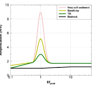
The four amplification functions are plotted together in Figure 2-8. In this plot,
the sediment amplification functions have their Apeak values normalized to an f/fpeak value
of 1, but the bedrock function is not normalized (i.e., it is plotted versus frequency in Hz).
The Apeak values of the till, sand/clay and organic amplification functions are 3.0, 5.2 and
9.0, respectively. These are slightly larger Apeak values than those seen in the H/V ratios
for Japan in Ghofrani and Atkinson (2014), possibly due to stronger velocity contrasts at
the base of the profile in Ontario; however, the overall shapes are similar in ENA and
Figure 2-8: Comparison of site amplification functions for different surficial geology
types. Till, sand/clay and very soft sediment/fill are plotted with respect to
normalized frequency.
2.5
Amplification Functions for Sites with Unknown Peak
Frequencies
The amplification functions obtained in the previous section were derived from
ground-motion recordings collected at seismograph sites. We focused on the
seismographic data due to the stability of the H/V spectra when gathered over multiple
earthquake recordings. Moreover, it is particularly important to understand site
amplification at seismographic sites, as this allows us to interpret seismographic data to
amplification functions are applicable for sites where the H/V ratios (or fpeak values) are
known with confidence. For most locations, however, we have only an estimate of fpeak
based on other information such as the sediment type and estimated depth-to-bedrock
(e.g., such as from the OGS sediment thickness map in Ontario). As mentioned
previously, the estimated depth-to-bedrock contains some uncertainty, and interpolating
for sites between coordinates for which such information is available introduces more
uncertainty. Only some of this uncertainty (excluding the component due to interpolation
between locations) is represented in the standard deviation of equation (2.1), which gives
fpeak to within a factor of ~1.6. Thus, we can say that our uncertainty in the estimate of
fpeak for sites without a direct measurement based on H/V is at least a factor of 1.6, and is
probably closer to a factor of two. A realistic model of site amplification across the
region for use in ShakeMap or similar applications must account for this uncertainty.
If we are uncertain as to the peak frequency of response, it is preferable to assume
a more generic amplification in which we have smoothed and broadened the peak over a
range of frequencies, as well as making it gentler in amplitude. This will also help
account for event-to-event variability in amplification at a site. To develop a smoothed
broad-peak function, we consider the implications of one standard deviation in the value
of fpeak (0.2 log units). For each sediment class’s normalized average H/V curve, a Monte
Carlo simulation is performed to generate 1000 identically-shaped curves, with random
variability in fpeak within 0.2 log units (assuming a normal distribution in log frequency
space). The average of these 1000 simulated curves is computed, which generates a curve
that has a broadened peak. To capture the overall trend of this average curve, we alter the
parameters of the Gaussian function from Ghofrani and Atkinson (2014). The results for
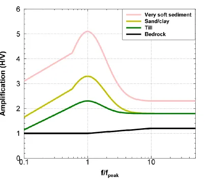
this process for the three sediment classes are shown in Figure 2-9 and the equations
which describe the broad-peaked sediment amplification functions are given by equations
(2.9) to (2.11). Since bedrock spectra have no peak frequency, the same function given by
equation (2.8) also applies here.
ATill(f/fpeak) = 1.25X + 2.39, f/fpeak < 0.6 (2.9a)
ASand/clay(f/fpeak) = 1.5X + 3.15, f/fpeak < 0.6 (2.10a)
ASand/clay(f/fpeak) = 1.5exp(-(X/0.38)2) + 1.8, f/fpeak ≥ 0.6, (2.10b)
AOrganic(f/fpeak) = 1.5X + 4.6, f/fpeak < 0.6 (2.11a)
AOrganic (f/fpeak) = 2.8exp(-(X/0.4)2) + 2.3, f/fpeak ≥ 0.6, (2.11b)
where X = log(f/fpeak), and we impose the condition that Amin = 1.
Figure 2-9: Suggested amplification functions for generic sites with poorly-known
2.6
Comparisons with a Typical Site Response Model Used
in California
An interesting aspect of the amplification functions in Figure 2-9 is that, even
after broadening and dampening the peaks by considering an uncertainty of a factor of
1.6 in fpeak, the inferred average amplifications on sediments in eastern Canada are still
much sharper and more pronounced than would be suggested by typical amplification
functions that are applied in western North America. For example, a typical western site
amplification model, derived from the NGA-West 2 database using VS30 as the site
variable, is that given by Seyhan and Stewart (2012). By assuming weak-motion peak
ground accelerations (PGAs) of 0.02g and a suitable, generic VS30 value for each type of
deposit, we can compare the site amplification functions for southern Ontario to those of
Seyhan and Stewart (2012), as shown in Figure 2-10. To make these comparisons, we
assume nominal values for VS30 of 1000 m/s for till, 300 m/s for sand/clay and 150 m/s
Figure 2-10: The three proposed generic sediment amplification functions for
eastern Canada and the corresponding functions for California (Seyhan and
Stewart, 2012) assuming nominal values of VS30 of 1000 m/s, 300 m/s and 150 m/s for
till, sand/clay and soft soil, respectively. Light shades refer to very soft sediment/fill;
intermediate to sand/clay; dark to till.
Note that till sites have, on average, high peak frequencies, while sand/clay sites
have intermediate peak frequencies. Sites in western North America (primarily California
data) have more subdued amplification profiles, with lower and broader peak frequencies,
reflecting more gradational sediment profiles. The only sites in eastern Canada which
could appear to have similar site amplification characteristics to the California functions
are soft, deep sites with low peak frequencies. By contrast, most sediment profiles in
eastern Canada are soft to stiff sediments of variable depth overlying much harder rock,
Stewart (2012) amplification functions were derived without consideration of the depth
of the deposit; this has the effect of broadening the functions (similar to how the
broad-peaked amplification functions for eastern Canada were derived). The difference seen in
Apeak between the California functions and the H/V spectra for eastern Canada may be
due partly to this broadening effect, and partly due to the higher impedance contrast in
eastern Canada. One may also infer from the low peak frequency of the California
sediment amplification functions, over all values of VS30, that the California model is
generally applicable to deep, gradational sites.
2.7
Summary and Conclusion
A preliminary site amplification model is developed for eastern Canada based on the
two predictive variables of fpeak and surficial geology type (bedrock, till, sand/clay,
very soft organic sediment/fill). The intended use of this model is to predict levels of
site amplification in a generalized sense, for application onto a real-time ShakeMap
product for the region. More detailed studies, based on more subsurface geological
information and velocity measurements in the field, are needed to refine this model.
The value of fpeak in the site amplification model is a function of depth-to-bedrock.
Similarly, Apeak is a function of surficial geology, or sediment stiffness. Sites in many
parts of eastern Canada have pronounced amplification around a peak frequency, due
to the sharp velocity contrast at the base of the profile.
For use in ground-motion mapping applications, it is necessary to consider
uncertainty in the value of fpeak. This uncertainty subdues and broadens the expected
value of the amplification (by averaging over a range of fpeak). However, the functions
are still sharper and more pronounced than in classic models for western regions.
The use of sediment thickness and surficial geology as a way to characterize site response in Ontario is convenient since these data are readily available and correlate
of sites in the region, unlike data for VS30, which are scarce and only inferred for
many seismograph stations.
H/V spectra in eastern Canada have high values of Apeak; however, these apply to
linear site amplification for weak-motions. Nonlinearity would be expected to
dampen these amplifications and shift the peaks to lower frequencies.
References
Aki, K and Richards, P.G. (2002). Quantitative Seismology, 2nd edition.University
Science Books. Sausalito, California. 700.
Assatourians, K. and Atkinson, G.M. (2008). Program: ICORRECT. Engineering
Seismology Toolbox. Department of Earth Sciences, The University of Western
Ontario. 40.
Atkinson, G.M. (2004). Empirical Attenuation of Ground-Motion Spectral Amplitudes in
Southeastern Canada and the Northeastern United States. Bulletin of the
Seismological Society of America, 94, 3, 1079–1095.
Atkinson, G.M. and Assatourians, K. (2010). Attenuation and Source Characteristics of
the 23 June 2010 M 5.0 Val-des-Bois, Quebec, Earthquake. Seismological
Research Letters, 81, 849–860.
Bard, P-Y. (1999). Microtremor measurements: a tool for site effect estimation? In:
Irikura, K., Kudo, K., Okada, H., and Satasini, T., (eds) The Effects of Surface
Geology on Seismic Motion. Balkema, Rotterdam, p. 1251–1279.
Chouinard, L. and Rosset, P. (2012). On the Use of Single Station Ambient Noise
Techniques for Microzonation Purposes: the Case of Montreal; in Shear Wave
Velocity Measurement Guidelines for Canadian Seismic Site Characterization in
Soil and Rock, (ed.) J.A. Hunter and H.L. Crow; Geological Survey of Canada,
Open File 7078, p. 85–93.
Vertical Response Spectral Ratios of Earthquakes in the NGA-West 2 and
Japanese Databases. Bulletin of Soil Dynamics and Earthquake Engineering, 67,
30–43.
Kawase, H., Sánchez-Sesma, F.J. and Matsushima, S. (2011). The Optimal Use of
Horizontal-To-Vertical Spectral Ratios of Earthquake Motions for Velocity
Inversions Based on Diffuse Field Theory for Plane Waves. Bulletin of the
Seismological Society of America, 101 (in press).
Kolos, D. (2010). Using Horizontal-to-Vertical Spectral Ratios to Estimate Shear Wave
Velocities of Soil at South-Eastern Canadian Seismological Stations. The
University of Western Ontario. Accelerated Master’s Thesis. 64.
Kramer, S.L. (1996). Geotechnical Earthquake Engineering. Prentice-Hall, Inc. Upper
Saddle River, New Jersey. 653.
Lermo, J. and Chávez-Garcìa, F.J. (1993). Site effects evaluation using spectral ratios
with only one station. Bulletin of the Seismological Society of America, 84, 1350–
1364.
Motazedian, D., Hunter, J.A., Pugin, A., and Crow, H.L. (2011). Development of a VS30
(NEHRP) Map for the City of Ottawa, Ontario, Canada. Canadian Geotechnical
Engineering Journal, 48, 3, 458–472.
Nakamura, Y. (1989). A method for dynamic characteristics estimation of subsurface
using microtremor on the ground surface. Quarterly Report of RTRI, 30, 25–33.
Pal, J. and Atkinson G.M. (2012). Scenario Shakemaps for Ottawa, Canada. Bulletin of
the Seismological Society of America, 102, 2, 650–660.
Rosset, P. and Chouinard L. (2009). Characterization of site effects in Montreal, Canada.
Natural Hazards, 48, 295–308.
Rosset, P., Bour-Belveaux, M., Chouinard, L. (2015). Microzonation models for
Montreal with respect to VS30. Bulletin of Earthquake Engineering, 13, 8, 2225–
2239.
Seyhan, E. and Stewart, J.P. (2012). Site Response in NEHRP Provisions and NGA
Models. Earthquake Engineering. 226, 359–379.
Seyhan, E. and Stewart, J.P. (2014). Semi-empirical nonlinear site amplification from