Bubble-Induced Inverse Gas-Liquid-Solid Fluidized Bed

(1)

Scholarship@Western

Electronic Thesis and Dissertation Repository

8-9-2017 12:00 AM

Bubble-Induced Inverse Gas-Liquid-Solid Fluidized Bed

Xiliang Sun

The University of Western Ontario

Supervisor Jesse Zhu

The University of Western Ontario

Graduate Program in Chemical and Biochemical Engineering

A thesis submitted in partial fulfillment of the requirements for the degree in Master of Engineering Science

Follow this and additional works at: https://ir.lib.uwo.ca/etd

Part of the Biochemical and Biomolecular Engineering Commons, and the Engineering Mechanics Commons

Recommended Citation Recommended Citation

Sun, Xiliang, "Bubble-Induced Inverse Gas-Liquid-Solid Fluidized Bed" (2017). Electronic Thesis and Dissertation Repository. 4754.

https://ir.lib.uwo.ca/etd/4754

This Dissertation/Thesis is brought to you for free and open access by Scholarship@Western. It has been accepted for inclusion in Electronic Thesis and Dissertation Repository by an authorized administrator of

(2)

i

Gas-liquid-solid fluidized beds have been widely applied in wastewater treatment, however, the current method of wastewater process has several limitations. Hence, an improved

method is in demand. A 3.5 height and 0.1534m inner diameter column was used to study the hydrodynamic characteristics of a bubble-induced three-phase inverse fluidized bed. Air, water and three types of low-density particles were employed as gas, liquid and solid phases.

The hydrodynamic properties in the bubble-induced three-phase fluidized bed were

investigated to provide the basic information for the industrial process, such as flow regime, bed expansion ratio and phase holdups. A flow regime map containing fixed bed, initial expansion, transition regime, complete fluidization and freeboard regime is presented. The bed expansion ratio behaves like the conventional fluidized bed. The axial profiles of the phase holdups show that with increasing gas velocity, liquid holdup has a downward trend, while gas holdup has an upward trend. Solids holdup is irrelevant with the gas velocity. Based on the Richardson-Zaki equation, a preliminary model between the solids holdup and superficial gas velocity was built.

Keywords

(3)

ii

Acknowledgments

I would like to take this opportunity to express the gratitude and appreciation to those who have always been helping and supporting me in the academic and daily life.

My sincerest thank to my Supervisor Dr. Zhu, for believing in my potential, supporting me not only on research but also on daily life during my whole period of master study, and setting a role model for me, which ensured my successful fulfillment of this study.

My gratefulness is directed to Tian Nan for being a good friend and his help designing and constructing the experimental equipment and the report problems.

Many thanks to my friends in the research group, Jiaqi Huang, Yingjie Liu, Yupan Yun, Bowen Han, Haolong Wang, Xiaoyang Wei and Danni Bao, for their help, advice and friendship.

I really appreciate Mr.Wen’s valuable advice in the experimental setups and George Zhang for his service.

Great gratitude is to my parents. Without their consistent and unreserved support, I could not have done this mission thus far a success.

Finally, my special thanks to my lovely boyfriend, Sida Zhou, for being the most

(4)

iii

List of Tables

Table 3.1 Measurement methods of main hydrodynamic parameters ... 22

Table 3.2 Physical properties of particles used in bubble-induced ITPFB. ... 27

(8)

vii

List of Figures

Figure 2.1 Simplified layout of wastewater treatment plant (WWTP). ... 4

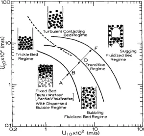
Figure 2.2 Flow regime diagram for a countercurrent gas-liquid-solid fluidized bed. Polyethylene hollow spheres, d=0.01m, ρs =388kg/m3; — liquid as a continuous phase, －－ gas as a continuous phase. ... 6

Figure 2.3 Flow regime map of inverse three-phase fluidized bed using small spherical particles, d=0.175mm, ρs=690kg/m3 (A) fixed or partially fluidized bed; (B) bubbling bed; (C)fluidized bed with the transition to coalescing bubble flow. ... 7

Figure 2.4 Schematic representation of the gas-liquid interface, concentration, mass transfer coefficients Kl, kl and kg according to two-film theory. ... 15

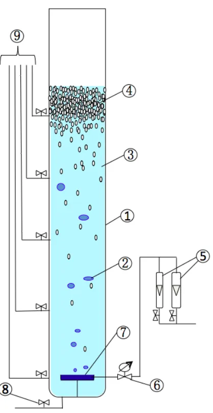
Figure 3.1 Schematic diagram of gas-driven inverse gas-liquid-solid fluidized bed. (1) column, (2) bubble, (3) liquid, (4) solid particles, (5) rotameters, (6) pressure gauge, (7) gas distributor, (8) liquid inlet/outlet valve, (9) manometer. ... 20

Figure 3.2 Picture of gas distributor. ... 21

Figure 3.3 Calibration curve of gas rotameter considering pressure gauge. ... 23

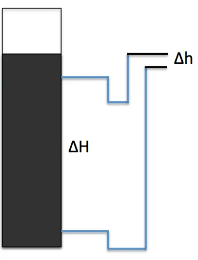
Figure 3.4 Schematic diagram of pressure drop through the column. ... 24

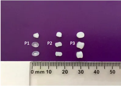
Figure 3.5 The appearance of three types of particles. ... 27

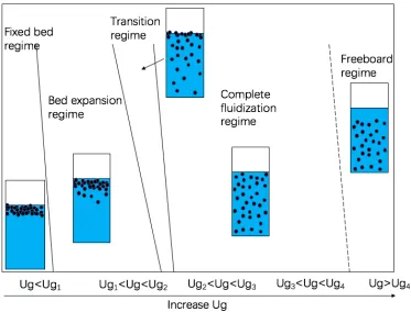
Figure 4.1 Flow regimes map in bubble-induced inverse three-phase fluidized bed. ... 29

Figure 4.2 Initial fluidization velocity (Ug1) as a function of solids loading for three types of particles. ... 30

(9)

viii

Figure 4.4 Complete fluidization velocity (Ug2) as a function of solids loading for three types

of particles. ... 33

Figure 4.5 Superficial gas velocity varied with particle’s densities. ... 34

Figure 4.6 Superficial gas velocity varied with solids loadings. ... 35

Figure 4.7 Superficial gas velocity varied with water level for three types of particles: (a) 904kg/m3_{, (b) 930kg/m}3_{and (c) 950kg/m}3_{. ... 37}

Figure 4.8 Superficial gas velocity varied with water level for three solids loadings: (a) 5%, (b) 10% and (c) 15%. ... 39

Figure 5.1 The selection of lowest layer of the expansion bed. ... 40

Figure 5.2 The variations of bed expansion ratio as a function of superficial gas velocity for three different particles: (a) 130cm, (b) 190cm and (c) 250cm. ... 43

Figure 5.3 The variations of bed expansion ratio as a function of superficial gas velocity for three water levels with three different particles: (a) 904kg/m3, (b) 930kg/m3 and (c) 950kg/m3. ... 46

Figure 5.4 The variations of bed expansion ratio as a function of superficial gas velocity for three solids loadings: (a) 130cm, (b) 190cm and (c) 250cm. ... 48

Figure 5.5 The variations of bed expansion percentage as a function of superficial gas

velocity for three solids loadings: (a) 130cm, (b) 190cm and (c) 250cm. ... 50

Figure 6.1 Schematic diagram of pressure drop through the column. ... 51

Figure 6.2 The variations of average phase holdups as a function of superficial gas velocity in two-phase (gas-liquid) system. ... 53

(10)

ix

Figure 6.4 Compare the average phase holdup in two-phase (gas-liquid) system and three-phase (gas-liquid-solid) system, ρs=930kg/m3, solids loading=15%. ... 55

Figure 6.5 The variations of average phase holdup as a function of superficial gas velocity for three different particles at solids loading = 15%: (a) gas holdup, (b) liquid holdup and (c) solids holdup. ... 58

Figure 6.6 The variation of average phase holdups as a function of superficial gas velocity for different loadings, ρs=930kg/m3: (a) gas holdup, (b) liquid holdup and (c) solids

holdup. ... 60

Figure 7.1 Compare the local phase holdup in two-phase (gas-liquid) system and three-phase (gas-liquid-solid) system, ρs=930kg/m3, solids loading=15%, from 130cm to

190cm. ... 63

Figure 7.2 The variations of local phase holdup as a function of superficial gas velocity for three different particles at solids loading = 15%: (a) 904kg/m3, (b) 930kg/m3 and (c) 950kg/m3. ... 65

Figure 7.3 The variations of height as a function of local solids holdup at different superficial gas velocity, solids loading = 15%, ρs=930kg/m3. ... 66

Figure 7.4 The variations of local solids holdup as a function of superficial gas velocity for three different particles, solids loading = 15%: (a) 10-70cm, (b) 70-130cm, (c) 130-190cm, (d) 190-210cm. ... 68

Figure 7.5 The variations of height as a function of local solids holdup for three different particles at solids loading = 15%: 904kg/m3, 930kg/m3 and 950kg/m3. ... 69

Figure 7.6 Compare the calculated local solids holdup and actual solids holdup ... 70

Figure 7.7 The variations of local solids holdup as a function of superficial gas velocity for different solids loadings, ρs=930kg/m3: (a) 10-70cm, (b) 70-130cm, (c)

(11)

x

Figure 7.8 The variations of height as a function of local solids holdup for five different solids loadings, ρs=930kg/m3. ... 73

Figure 8.1 A schematic diagram of the bubble-induced three-phase system. ... 75

Figure 8.2 Compare the average solids holdup in experiment and model system for different kind of particles: (a)904kg/m3_{, (b) 930kg/m}3_{. ... 78}

Figure 8.3 Compare the average solids holdup in experiment and model system for different solids loadings. ... 79

(12)

xi

List of Appendices

Appendix A Calibration curve for the gas rotameter ... 93

Appendix B Examples of error analysis ... 94

Appendix C Initial fluidization velocity, full expansion velocity and complete fluidization velocity ... 98

Appendix D Bed expansion ratio ... 100

(13)

Chapter 1

1

General Introduction

1.1 Introduction

Fluidization is solid particles are kept under suspension supported by the flow of fluid phase. At first, when the fluid is introduced into the static bed at a low velocity, fluid transits through the void between solid particles and particles remain as a static bed known as a fixed bed. The displacement of particles happens as increasing the fluid velocity, and it is known as an expanded bed. Now, particles are suspended with a higher velocity in the fluid and the drag force acts as a balancing force between the buoyancy and gravity. At a specific fluid velocity, the minimum fluidization velocity (Umf), the pressure drop through the bed is equal to the weight of the particles, which is a dynamic equilibrium. Under this situation, the bed is considered as a fluidized bed [Khan et al., 2014]. The phenomenon can be described as a mathematic equation [Yang, 2003]:

(1.1)

Fluidized beds have been used in many areas, especially in chemical and biochemical processing, like wastewater treatment. The efficient mixing and high mass/ heat transfer are the crucial factors in the fluidized bed [Bello et al., 2017].

Three-phase (Gas-liquid-solid) fluidized bed (TPFB) has been studied and it has many applications in chemical, petrochemical, pharmaceutical and biochemical industries [Fan,1989]. After employing particles, which density is lower than the liquid phase, as the solids phase, the fluidization system is known as an inverse three-phase fluidized bed (ITPFB). Compared to the conventional TPFB, the advantages of inverse fluidization contain simple reactor structure, convenient operation [Fan,1989], good fluidization at low fluid velocity, high rate of mass transfer [Fahim et al., 2013], high rate of heat transfer [Myre and Macchi, 2010] and effective control of biofilm thickness in

biochemical treatment [Sokół and Woldeyes, 2011; Campos-Díaz et al., 2012]. With the development of inverse fluidized system, certain hydrodynamic characters have been

(14)

investigated with solid experimental results, such as flow regime [Han et al., 2000], pressure drop, bed expansion [Bendict et al., 1998; Kim and Kang, 2006], minimum fluidization velocity [Das et al., 2015], phase holdups [Shin et al., 2007;] and bubble behaviors [Narayanan et al., 2014; Hamdad et al., 2007]. Some other hydrodynamic characters such as mass and heat transfer coefficient have also been studied [Garcia-Ochoa and Gomez, 2009; Myre and Macchi, 2010].

A detailed literature review of the hydrodynamic of inverse fluidized bed previous study has been shown in Chapter 2.

1.2 Objectives

In this thesis, the following objectives should be achieved:

1. Basic concepts of the bubble-induced inverse gas-liquid-solid fluidized bed are first discussed to give a general background of this new technology.

2. Important hydrodynamic parameters related to reactor design and processes are discussed. As significant hydrodynamic characters determine the effectiveness of the fluidization process, flow regimes, bed expansion, and axial phase holdups will be studied in this thesis.

3. Based on the Richardson-Zaki equation, a preliminary model for the solids holdup and superficial gas velocity will be built.

1.3 Thesis structure

This thesis is based on the hydrodynamic characters of the bubble-induced inverse gas-liquid-solid fluidized bed.

Chapter 1 introduces the theoretical basis of fluidization and (inverse) three phase fluidized bed followed by the detailed literature review of hydrodynamic characters and applications in Chapter 2.

(15)

According to different gas flow velocity, flow regimes can be separated as fixed bed regime, initial expansion regime, transition regime, complete fluidization regime and freeboard regime. The effects of the particle property and water level on transition gas velocities are studied in Chapter 4.

Chapter 5 is discussed about the effects of particles property and solids loading on the bed expansion ratio in the initial expansion regime and transition regime. While in the complete fluidization regime, the average phase holdups and local phase holdups were studied in Chapter 6 and Chapter 7, respectively.

Based on the Richardson-Zaki equation, a preliminary model related to the superficial gas velocity and phase holdup is introduced in Chapter 8. And some assumptions and

discussions also be presented.

The conclusions and recommendations in Chapter 9 are described some main results of the thesis and some suggestions of the future work.

(16)

Chapter 2

2

Literature review

2.1 Introduction

Cleaning up the important source of water is a task of top priority. In Canada, over 150 billion liters of untreated and undertreated wastewater discharge into the waterways every year. Water is the source of life, in other word, water quality and human health have a close relationship. The current technology used in wastewater treatment is shown in Fig 2.1 [Lacroix et al., 2014]. However, the drawback of this process is that it requires large area but has low efficiency and long processing time. In addition, the main parts of this technique are the primary and secondary process and the aeration part. With the city development and population growth, this technique could not offer the clean water requirement in the future. Therefore, a new technology of wastewater treatment is in demand.

Figure 2.1 Simplified layout of wastewater treatment plant (WWTP).

(17)

grow on the surface of particles, the microorganism will move with the particles, which means the effective reaction area is larger than the suspended one.

Meanwhile, the sheer stress among particles can control the thickness of the biofilm, therefore a good mass transfer efficiency is achieved. Since the inverse fluidized bed can control the biofilm in a narrow range compared with the conventional one, the inverse fluidized bed reactor is more suitable for the wastewater treatment. Moreover, in the bubble-induced inverse fluidized bed, particles are fluidized only by an upward gas flow, which means there’s no liquid flow in the system. Considering all kinds of situation, the bubble-induced inverse three-phase fluidized bed is employed as the new technology of wastewater treatment.

In inverse gas-liquid-solid fluidized bed, gas flows up and liquid goes downwards. Air, tap water and low-density particles are employed as gas phase, liquid phase and solids phase, respectively. As the density of particles is lower than the liquid, the particles floated on the top of the bed at first. After achieving the minimum fluidization velocity, the fixed bed disappears and the particles fluidize. Inverse fluidized bioreactors are employed in wastewater treatment in various industries [Nikolov and Karamanev, 1987; Karamanev and Nikolov, 1996]. Furthermore, some hydrodynamic characters in inverse fluidization have been studied to investigate the effects of different parameters.

2.2 Hydrodynamic characters in inverse fluidization

2.2.1 Flow regimes

(18)

regime, bed expansion ratio is influenced by the liquid velocity and gas velocity. At the constant liquid velocity, the bubble size and frequency do not change with increasing the gas velocity, however, the gas holdup through the bed increases while the liquid holdup decreases. Meanwhile, the sectional area of liquid decreases. On the other hand, at constant gas flow rate, increasing the liquid flow rate improves the linear liquid velocity, which encourages the particles to move with the liquid and leads to the initial expansion. The transition regime is narrow and difficult to control. The specialty in this regime is that bubbles become coalescence and the bubble size and frequency changes. In slugging fluidized bed regime, bubble impacts the particles, meanwhile, particles also have an influence on the bubble size and movement. The interaction effect between bubbles and particles occurs constantly.

Figure 2.2 Flow regime diagram for a countercurrent gas-liquid-solid fluidized bed. Polyethylene hollow spheres, d=0.01m, ρs =388kg/m3; — liquid as a continuous

phase, －－ gas as a continuous phase.

(19)

Figure 2.3 Flow regime map of inverse three-phase fluidized bed using small spherical particles, d=0.175mm, ρs=690kg/m3 (A) fixed or partially fluidized bed;

(B) bubbling bed; (C)fluidized bed with the transition to coalescing bubble flow.

2.2.2 Pressure gradient

Pressure gradient is one of the significant parameters to calculate the energy and power expenditure. Briens et al. reported the minimum fluidization liquid velocity (Ulmf) can be obtained by measuring the static pressure drop through a three-phase inverse fluidized bed [Briens et al., 1997]. With the basic principle of inverse fluidization, the pressure gradient through the bed is equal to the density of bed multiplies gravitational

acceleration. Eq.2.1 expresses the pressure gradient in inverse three-phase (gas-liquid-solid) fluidized bed; the frictional pressure gradient in inverse two-phase (liquid-(gas-liquid-solid) fluidized bed has represented in Eq.2.2.

−ΔP Δz ⎛ ⎝

⎜ ⎞

⎠ ⎟

bed

=ρbedg=

(

ρsεs+ρlεl+ρgεg

)

g (2.1)

−ΔP Δz ⎛ ⎝

⎜ ⎞

⎠ ⎟

f,ls

=εs(ρs−ρl)g (2.2)

(20)

−ΔP Δz ⎛ ⎝ ⎜ ⎞ ⎠ ⎟ bed

=

(

εs+εl

)

ρlg+εgρgg+ −

ΔP Δz ⎛ ⎝ ⎜ ⎞ ⎠ ⎟ f,ls (2.3)

However, a different consequence can be acquired by assuming the force on the solid

parts is provided by the liquid-gas mixture [Lee et al., 2000]. For a fixed bed, −ΔP Δz ⎛ ⎝ ⎜ ⎞ ⎠ ⎟

f,ls

can be expressed by the Ergun equation [Ergun, 1952], then applied to the two-phase interaction. Neglecting the term εgρgg in Eq2.3, a final representation of pressure

gradient is given below

1 ρlg −

ΔP Δz ⎛ ⎝ ⎜ ⎞ ⎠ ⎟ bed

=1−εg−150εs 2

µlU_l Φ2dp

2

εl3ρlg−

1.75εsU_l2

εl3Φdpg

(2.4)

Buffière and Moletta found 4 parameters a,b,c,d to fit the experimental data for the collision frequency and particle pressure under the given equation [Buffière and Moletta, 2000]:

(2.5)

The optimum values obtained are

a=305700,b=1.01(≈1),c=1.02(≈1),d=0.99(≈1) for collision frequency;

a=423,b=1,c=1.14,d=0.75 for the dimensionless particle pressure.

2.2.3 Minimum fluidization velocity

Minimum fluidization velocity is one of the conclusive parameters for the design of the three-phase fluidized bed [Zhu et al., 2007]. The definition is when the pressure gradient through the bed reaches the minimum, the superficial velocity is the minimum liquid fluidization velocity (Ulmf) [Cho et al., 2002]. In addition, the minimum liquid

fluidization velocity also can be measured when the drag force balances the gravity and buoyancy of the particle [Lee et al., 2000].

Model=a F εs

εs0

⎛ ⎝ ⎜ ⎞ ⎠ ⎟ ⎡ ⎣ ⎢ ⎤ ⎦ ⎥ b Ug c εs

εs0

(21)

Lee reported although Ulmf decreases as gas velocity increases, the patterns sometimes

display concave-downward, sometimes concave-upward and sometimes S-shape behavior. The difference may be caused by the effects of liquid motion induced by rising bubbles and solids agglomerates attached to bubbles. Furthermore, Ulmf with wetting agent is

lower than Ulmf without wetting agent, this phenomenon is attributed to the wetting agent

that is effective to eliminate the bubble attached to the particles [Lee et al., 2000]. Das investigated with four different type particles and four different concentration non-Newtonian liquids and obtained that with increasing the bed weight, the pressure drop increases, however, the minimum inverse fluidization velocity is almost constant, which means the Ulmf is independent of solids loading. Meanwhile, Ulmf has no relevance with

the column diameter. Ultimately, Das summarized that Ulmf is only determined by

Reynolds number (Re) and Archimedes number (Ar) and particle properties (such as particle size, density, and sphericity) [Das, 2010].

2.2.4 Phase holdups

Phase holdup is one of the important hydrodynamic characteristics of the three-phase fluidized bed, which decides the fluidization efficiency within the fluidized bed. At present, the measurements of different phase holdups are various.

The well-established method of calculating the solids holdup is given below

(2.6)

Fan reported that in the inverse bubbling regime the liquid flow rate on gas holdup (εg)

could be neglected. By comparison, in the conventional three-phase fluidized bed with large particles, the gas holdup decreases with an increasing liquid flow rate. Additionally, in the inverse slugging fluidized regime, the gas holdup has an opposite trend compared with the conventional bed. The empirical equations of the gas holdup in inverse bubbling regime and inverse slugging regime are given by [Fan et al., 1982a]:

εg =0.322ε 1.35

(U_go/U_l₀)0.18 (2.7) εs=

M

π

4dp 2

(22)

for the inverse bubbling fluidized bed regime and

εg =2.43Ug0 0.704_U

l0

0.25_(2.8)

for the inverse slugging fluidized bed regime.

Furthermore, Shin et al. suggested that the variation of liquid holdup is complex, gas holdup and solids holdup decreases with increasing the liquid viscosity. In addition, Shin et al. summarized that the physical properties and operating conditions then got some corrected equations of gas holdup and liquid holdup. Meanwhile, an equation related the solids holdup calculation is also given below [Shin et al., 2007]

εg =5.517Ug

0.383_U

l

0.426

µl −0.071₍ρs

ρl

)11.357_(2.9)

εl=4.014Ug

0.136_U

l

0.155

µl

0.056₍ρs

ρl

)2.009_(2.10)

1−εs =5.568Ug

0.158_U

l

0.169

µl

0.048₍ρs

ρl

)2.762_(2.11)

Kim and Kang studied the bubble parameters and got gas holdup correlated as [Kim and Kang, 2006]

εg =1.18Ug

0.235_U

l

0.335

µl

0.391₍ρs

ρl

)3.61_(2.12)

(23)

variation of phase holdups in the bed is rather than assuming an average phase holdup of the entire bed [Bandaru et al., 2007].

Unfortunately, as the local holdup is related with lots of influencing factors, the accurate value is not easy to measure, thus there are a few related articles written about the local holdup studies.

2.2.5 Bed expansion

The general definition of fluidized bed expansion ratio is the ratio of bed height after the expansion and initial bed height. The bed expansion ratio can speculate the

hydrodynamic in fluidized bed after change operating conditions. Bed expansion is a complex parameter affecting various kind of fluid mechanics. Furthermore, if bed expansion can be predicted by equations, it would be useful in actual operation design.

Despite bed expansion is important in fluidized bed design, not much of work has been reported in the literature for the detail experiments. Sau et al. have developed several empirical equations for bed expansion ratio in gas-solid tapered fluidized bed. The models for different types of particles were obtained and are given as follows [Sau et al., 2010].

For spherical particles:

R=2.811(D0 D₁)

0.05 (hs

D₀)

−0.027 (dp

D₀)

−0.463 (ρs

ρf )−0.236

(U−Umf U_mf )

0.157_(2.13)

and for non-spherical particles:

R=10.967(D0

D1

)0.119(hs D0

)−0.233

(dp

D0 )−0.091

(ρs ρf

)−0.225

(U−Umf

Umf

)0.261 (2.14)

(24)

U Ui

=εn (2.15)

Fan et al. studied the bed expansion of inverse fluidized bed based on R-Z equation and got the n values equations [Fan et al., 1982a]

n=15Re−0.35_e3.9

dp

D (2.16)

for 350 < Re < 1250, and

n=8.6 Re−0.2_e−0.75 dp

D _(2.17)

for Re > 1250. The article does not mention about how to determine the superficial fluid velocity Ui, but supposedly this has been done using the well-known standard drag curve.

2.2.6 Particle property

There’s no author considering the particle property effect on fluidized efficiency. Therefore, after analyzing the data the articles mentioned, some conclusion can be obtained.

The particles with a density close to liquid required lower minimum fluidization velocity, which can be explained that particles move with liquid and smaller density difference results in less energy required to support the fluidization of particles [Buffière and Moletta, 1999].

2.2.7 Bubble behaviors

Bubble behaviors are one of the important parameters in three-phase fluidized bed research and design, which can be used for bed operating regime division and determine the flow structure. Bubble behavior directly determines the axial-radial phase holdup in the bed distribution, interaction and interphase heat and mass transfer efficiency.

(25)

2014]. Bubble rising velocity increases with increasing superficial gas velocity or

increasing liquid viscosity; decreases when the superficial liquid velocity increases [Kim and Kang, 2006; Son et al., 2007]. Bubble rising velocity has a positive correlation with the solids loading [Son et al., 2007]. Bubble frequency has a positive correlation with flow superficial velocity, while has a negative correlation relationship with liquid viscosity [Kim and Kang, 2006; Son et al., 2007]. Son et al. studied and found that bubble size, bubble rising velocity and frequency has been well correlated based on the concept of gas drift flux by means of dual electrical resistivity probe system. The equations are given by [Son et al., 2007].

L_b=0.117(Ug+Ul 1−εg )

0.446 (ρs

ρl)

−2.78

µl0.191 (2.18)

Ub=0.108(

U_g+U_l 1−εg

)−0.219 (ρs

ρl

)−2.98 µl

0.076_(2.19)

Fb=30.846(

Ug+Ul 1−εg

)0.404 (ρs

ρl )6.732

µl

−0.002_(2.20)

Hamdad et al found that adding surfactants (ethanol) can reduce the minimum superficial gas velocity, inhibit bubble coalescence and decrease bubble rising velocity,

consequently, increase gas holdup. The principle is same as adding surfactants in a conventional three-phase bed [Hamdad et al., 2007]. However, different surfactants have various influences on bubbles. For the larger bubbles, additives like sodium chloride (NaCl), sodium phosphate dibasic (Na2HPO3) and benzoic acid reduce the gas holdup. A

possible explanation was given by Briens et al., who stated that the additives stabilize bubbles surfaces, inhibiting the splitting caused by shear force, as a result, reduce gas holdup. In conclusion, the surfactant has two main fractions: one is inhibiting bubble split which reduces gas holdup, while the other one is inhibiting bubble coalescence which increases gas holdup [Briens et al., 1999].

(26)

types of gas distributor, column diameter and pressure gradient may affect the bubble behaviors, while, the articles about this field are not getting much attention recently.

2.2.8 Residence time distribution (RTD)

Residence time distribution can reveal the existing problems on the reactors then improve the design of the reactor. However, this area doesn’t draw much attention.

Sánchez et al. investigated the fraction influence on residence time distribution and liquid mixing within a tracer used as a solution of potassium chloride (KCl). RTD curves with different solids fractions are presented in the dimensionless form E(θ) [Sánchez et al., 2005].

E(θ)= C(θ)

(Q/V)

∑

CiΔti

= C(θ)

(

∑

CiΔti)ta

(2.21)

where

θ=t/ta (2.22)

2.2.9 Mass transfer property

The internal mass transfer between reactor and substance is one of the important

parameters in design and industries application. Inverse three-phase fluidized bed mainly includes the gas-liquid phase mass transfer and liquid-solid phase mass transfer.

In aerobic bioprocessing, oxygen is the key part as its low solubility in aqueous solutions but a continuous supply is needed. Mass transfer of gas-liquid interface is a complicated process, which is strongly influenced by the hydrodynamic conditions in the reactor. The mass transfer coefficient (k_L) can be estimated by many equations. Some of them are

(27)

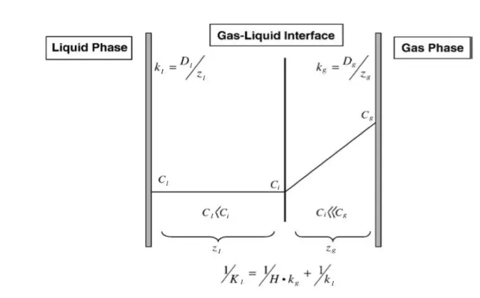
In inverse three-phase fluidized bed, Whitman’s two-film model is used widely (Fig.2.4). For the low-solubility gas (oxygen) and liquid interface mass transfer, the oxygen mass transfer rate per unit of reactor volume, NO2, is obtained by the product of overall flux

and the gas-liquid interfacial area per unit of liquid volume, a.:

(2.23)

In this equation, due to the oxygen is soluble in water slightly, the Henry constant H is very high. It is commonly accepted that the resistance on the liquid side of the interface is more than in the gas side, thus the resistance on the gas side can usually be neglected. Combined Eq2.19, the overall mass transport coefficient (Kl) is equal to the local

coefficient (kl).

1 K_l =

1 Hk_g +

1

k_l (2.24)

Figure 2.4 Schematic representation of the gas-liquid interface, concentration, mass transfer coefficients Kl, kl and kg according to two-film theory.

Meanwhile, because of the difficulty of measuring kland a separately, the product kla can

be measured instead of two factors called volumetric gas-liquid mass transfer coefficient.

NO₂ =aJ=kla(C

(28)

Hamdad et al. reported that kla has a positive relationship with gas velocity but do not

have a significant change in liquid velocity. Increasing gas velocity enhanced gas holdup and intensity of turbulence, while liquid velocity has little effect on bubble coalescence and gas holdup. Moreover, increasing solids loading decreases values of kla at gas

velocities over 20mm/s. This phenomenon is primarily due to decrease the gas holdup then a decrease in a happens [Hamdad et al., 2007].

Fahim observed that kla is proportional to superficial gas (up to175%) and liquid velocity

(up to 24%) both in a model and real fermentation conditions. Furthermore, the oxygen transfer in inverse three-phase fluidized bed is higher than in other bioreactors. And combined different conditions, an empirical equation is given by [Fahim, 2013]

kla(

µg ρgg2)

1

3₌_4.345*10−7

ug( ρg

µgg

) 1 3 ⎡ ⎣ ⎢ ⎢ ⎤ ⎦ ⎥ ⎥ 0.526

ul( ρg

µgg

) 1 3 ⎡ ⎣ ⎢ ⎢ ⎤ ⎦ ⎥ ⎥ 0.446

σ( ρg

µg 4 g) 1 3 ⎡ ⎣ ⎢ ⎢ ⎤ ⎦ ⎥ ⎥ 0.579 (2.25)

2.2.10 Heat transfer property

Temperature control is the key part of reactors not only controlled temperature can maintain the optimal reaction rate, but also temperature can affect the fluid property like density, viscosity, and diffusivity. In addition, temperature also has an influence on microorganisms that need a compatible environment to live and grow. In a word, the understanding of heat transfer phenomenon is necessary for industrial applications. Heat transfer coefficient (h) is investigated to perform the character of surface-to-bed or wall-to-bed heat transfer.

The immersed heater-to-bed heat transfer coefficient is measured when flow velocity is higher than the minimum fluidization velocity. The heat transfer increases with an

(29)

With liquid velocity inverse three-phase fluidized bed,

Nu=hdp(1−εs)

klεs

=0.084(Cpµl kl

)(dpρlUg µlεs

)0.944 (2.26)

without liquid velocity inverse three-phase fluidized bed,

Nu=hdp(1−εs)

klεs

=0.050(Cpµl kl

)(dpρl(Ug+Ul) µlεs

)0.810

(2.27)

Average surface-to-bed heat transfer coefficient increases with gas velocity, same as the heater-to-bed heat transfer coefficient. Since bubble size and bubble rising velocity increases with gas velocity, which enhances the turbulence through the bed. Average heat transfer coefficient increases at low solids loadings, however, decreases after a point of solids loading. This trend is related to the probe surface renew frequency. Increasing solids loading means more contact between particles and fluid, which results in a higher rate of fluid transfer around the probe. Above that point of concentration, higher solids loading of the liquid-solid phase causes an apparent viscosity increase, hence, the heat transfer coefficient decreases. Combined various parameters, Son et al got an

experimental Nusselt number equation which is confirmed by Myre and Macchi ’s experiment [Myre and Macchi, 2010].

h=C klρlCpl

[(Ul+Ug)(ρlεl+ρgεg+ρsεs)−(Ugρg)]g

εlµl ⎧ ⎨ ⎩ ⎫ ⎬ ⎭ 1 2 ⎡ ⎣ ⎢ ⎢ ⎢ ⎤ ⎦ ⎥ ⎥ ⎥ 1 2 (2.28)

Nu=hdp(1−εs)

k_lεs

(30)

2.3 Hydrodynamic characters in bubble-induced inverse

three-phase fluidized bed

(31)

Chapter 3

3

Experimental apparatus and measurement methods

3.1 The structure of bubble-induced inverse gas-liquid-solid

fluidized bed

A schematic diagram of the bubble induced inverse gas-liquid-solid fluidized bed is shown in Fig 3.1. A PVC column was employed as the main part with 0.1524m inner diameter and 3.5m height. Air, tap water and low-density particles were employed as gas, liquid, and solids phase, respectively. In addition, solids phase included three types of particles, including 904kg/m3 _{polypropylene, spheroid; 930kg/m}3_{polyethylene, cylinder;}

(32)

Figure 3.1 Schematic diagram of gas-driven inverse gas-liquid-solid fluidized bed. (1) column, (2) bubble, (3) liquid, (4) solid particles, (5) rotameters, (6) pressure

gauge, (7) gas distributor, (8) liquid inlet/outlet valve, (9) manometer.

3.2 Experimental procedure

To avoid the possibility of air binding which results in the sudden break, the gas velocity decreases after complete fluidizing at high gas velocity.

(33)

At first, the liquid was introduced from the inlet valve to the column until the determined height. As there’s no water release, the liquid inlet/outlet valve should remain close during the experiment. Then, premeasured particles were added through the top of the column. Air was measured with the gas rotameters before being introduced through the gas distributor. Two different range gas rotameters were used to satisfy various operating conditions.

The solids concentration also called solids loadings were determined by the ratio of static bed height (H0) to total height of column (Htotal), varying from 5% to 20% (volume

fraction).

Moreover, gas distributor was made of porous quartz with an 8.7cm outer diameter and a 2.7cm inner diameter (Fig3.2). The bubbles are small by using porous quartz, which can guarantee the good fluidization in the system. In addition, a pressure gauge was

connected between the rotameters and gas distributor to measure the inlet gas pressure.

(34)

3.3 Measurement procedures

Main hydrodynamic parameters measured in this study includes superficial gas velocity (Ug), pressure drop, average phase holdups (ε), local solids holdup (εs), bed expansion

ratio (R) and so on. The measuring devices are listed in Table 3.1.

Table 3.1 Measurement methods of main hydrodynamic parameters

Parameters Measuring devices

Superficial gas velocity Gas rotameter, pressure gauge

Pressure drop Pressure taps, manometer

Average phase holdups Pressure taps, manometer

Local solids holdup Pressure taps, manometer

Bed expansion ratio Photography

3.3.1 Measurement of superficial gas velocity

The superficial gas velocity is measured by the gas rotameter combined with the pressure gauge between rotameter and gas distributor.

After combined the pressure gauge, the calibrated gas flow rate was calculated by the following equation

PacVac =nRT (3.1)

PstVst=nRT (3.2)

the term of “nRT” is same in Eq3.1 and Eq3.2, then Vaccan be obtained by

Vac= PstVst

(35)

Furthermore, as gas flow rate is related to the column diameter, superficial gas velocity is used instead of the gas flow rate. Superficial gas velocity is an artificial one, which is calculated under the hypothesis that gas is the only one flowing in the given cross section area. Superficial gas velocity is calculated by the following equation.

Ug= Q_g π

4D 2

(3.4)

There’s common that Pac is equal to 1atm, under the circumstance, Vac(1atm) was shown

in Fig 3.4. Pst increases with increasing gas velocity, so, the slope in Fig3.4 has an

upward bend.

Figure 3.3 Calibration curve of gas rotameter considering pressure gauge.

3.3.2 Measurement of pressure drop

Pressure drop is measured by the equal mounted pressure taps and manometer. Photographs are employed for calculating the different height as they can record the

0 10 20 30 40 50

(36)

height within extremely short time to decrease the impact of water level fluctuates. Besides, the use of image, not only the time differences but also the personal reading errors are reduced.

Moreover, to minimize the personal reading errors, three images are taken to get the average pressure drop.

3.3.3 Measurement of average phase holdups

Average phase holdup is studied in the complete fluidization regime. To calculate the average phase holdups, a pressure balance between the top pressure tap and bottom pressure tap is given as

ρlgΔh+ρmgΔH=ρlgΔH (3.5)

Figure 3.4 Schematic diagram of pressure drop through the column.

Meanwhile, mixture of gas, liquid and solid phase can be calculated by

(37)

and it is known that the amount of adding three phase holdups is equal to one.

εs+εl+εg=1 (3.7)

Liquid was added when decrease gas velocity to remain the total bed height unchanged (visually), thus pressure taps are measured the pressure difference in fixed height through the column. The amount of added liquid is recorded to calculate the average liquid

holdup.

εl=

V_water

V_bed (3.8)

Therefore, with four equations and four unknown variables, column mixture density can be expressed by pressure drop, while gas holdup (εg) and solid holdup (εs) can use liquid

holdup (εl) and column mixture density to calculate.

εg =

(ρs−ρm)−(ρs−ρl)εl

(ρs−ρg)

(3.9)

εs=

(ρm−ρg)+(ρg−ρl)εl

(ρs−ρg)

(3.10)

3.3.4 Measurement of local phase holdups

For the local phase holdups, the main assumption of this model is that the axial liquid distribution in the column is uniform, which means the local liquid holdup is equal to the average liquid holdup.

(3.11)

Gas holdup (εg) and solids holdup (εs) can be obtained by the same equation of average

phase holdups.

(38)

3.4 Particle properties

The physical properties of the 3 types of particles employed in bubble-induced ITPFB are shown in Table 3.2. The density of particles is determined by the average of 50 samples. The appearance of particles shown in Fig 3.6. The terminal particle velocity is

determined by the following equation (Karamanev, 1996):

(3.12)

for free rising particles,

(3.13)

for (3.14)

(3.15)

for (3.16)

(3.17)

Ut=

4(ρp−ρl)gdp 3ρlCD

CD= 432

Ar (1+0.0470Ar

2

3₎₊ 0.517

1+154Ar

1 3

Ar<1.18*106 dp

2

C_D=0.95

Ar>1.18*106dp 2

Ar=gdp

3

ρl(ρl−ρp)

(39)

Figure 3.5 The appearance of three types of particles.

Table 3.2 Physical properties of particles used in bubble-induced ITPFB.

Particles Shape ρs(kg/m3)

ε

Sphere Φ dp (mm) Ut (cm/s)

P1 Spheroid 904 0.359 0.988 3.5 6.74

P2 Cylinder 930 0.353 0.841 3.5 5.73

(40)

Chapter 4

4

Experimental investigation of flow regimes

In an inverse three-phase fluidized system, the liquid is considered as continuous phase while gas is the dispersed phase, generally. Based on the experimental phenomenon and some literature about the gas velocity definition [Fan et al., 1982b, Buffière and Moletta, 1999], three transitional gas velocities have been recorded as initial fluidization velocity (Ug1), full expansion velocity (Ug2) and complete fluidization velocity (Ug3).

Based on the experimental phenomenon, different flow regimes are presented depending on different gas velocities. The main method to analyze the flow regimes was visual observation. A schematic representation of the flow regimes with different gas velocities is shown in Fig 4.1. At first, particles, which densities are lower than liquid’s density, were fixed at the top of the column when there’s no gas flow rate. After the gas was introduced through the gas distributor, the lowest fixed particles began to fluidize. This gas velocity is called as initial fluidization velocity (Ug1). When superficial gas velocity

was beyond Ug1, packed bed was gradually broken from the bottom to the top. The

transform was too fast to control, therefore an initial fluidization velocity was used to instead of the minimum fluidization velocity that was the minimum superficial gas velocity required to keep all particles in action. With continuing increasing the gas velocity, particles were full distributed through the whole column. However, the solids distribution was not uniform in this regime. Some particles can reach the bottom, while most particles were fluidized at the top. In other words, solids concentration was

diminishing from the top to the bottom through the column gradually. In this regime, full expansion velocity (Ug2) was achieved when some particles reached the bottom of the

column. With further increasing the gas velocity, the difference of the solids

concentration was reduced then disappeared, which means solid particles were uniformly distributed through the column with higher gas velocities, while the minimum gas

velocity to maintain this situation is known as complete fluidization velocity (Ug3).

(41)

distributed through the bed again, while only gas and liquid still existed at the top of the column when superficial gas velocity was beyond top freeboard velocity (Ug4). As the

value of Ug4 was higher than the velocity range in this project, the detailed investigation will be studied in the future.

The effects of particle properties and solids loadings on three specific gas velocities were discussed in the following parts.

Figure 4.1 Flow regimes map in bubble-induced inverse three-phase fluidized bed.

4.1 Initial fluidization velocity (

U

g1

)

Initial fluidization velocity is the minimum superficial gas velocity required to break the fixed bed, while the particles in the lower position begin to fluidize. The variations of the initial fluidization velocity (Ug1) with solids loadings for 3 types of particles are shown in

Fig 4.2. Initial fluidization velocity (Ug1) decreases with increasing the solids loading for

P2 (930 kg/m3_{) and P3 (950 kg/m}3_{) because particles fluidization is controlled by the}

(42)

particle fluidization is indirectly controlled by gas flow rate. With increasing the solids loadings, more particles immerse into the water and the lowest particles are more closed to the gas distributor, which means easier to begin to fluidize. However, Ug1 for P1 (904

kg/m3_{) doesn’t decrease with increasing solids loadings, the reason is that P1 is easy to}

form an aggregation. Aggregation begins serious with increasing solids loading, which means P1 requires higher gas flow rate to break the aggregation. The required gas flow rate is higher than the diminished one caused by increasing solids loading.

Ug1 for P2 is lower than Ug1 for P3 though the density of P3 is closer to liquid density

than P2. Because the diameter of P3 is larger than the diameter of P2, the gas velocity of P3 required to fluidized is higher than P2 requirement, which means, at a same gas flow rate, P2 is easier to fluidize than P3.

Figure 4.2 Initial fluidization velocity (Ug1) as a function of solids loading for three types of particles.

0 1 2 3 4 5

0 5 10 15 20 25

U

g1

(m

m

/s

)

Solids loading (%)

904-3.5

930-3.5 950-4.6 ρs dp

kg/m3 _mm

P1

P3

(43)

4.2 Full expansion velocity (

U

g2

)

Full expansion velocity is the superficial gas velocity when some particles have reached the bottom of the column, however, the distribution of solids concentration is not uniform. The variations of the full expansion velocity (Ug2) with solids loadings for 3

types of particles are shown in Fig 4.3. For all particles, full expansion velocity (Ug2)

decreases then keeps constant with increasing solids loadings, because gas flow rate drives liquid movement which actuates particles fluidization indirectly. With increasing solids loading, more particles immerse into the water, which means the low-position particles are closer to the gas distributor. At same gas velocity, the particles begin to fluidize then reach the bottom, whereas, some particles still fix at the top of the bed. The drag force for each particle to reach the bottom is same, so, the Ug2 keeps constant with

increasing solids loadings when the required gas flow rate is obtained.

(44)

Figure 4.3 Full expansion velocity (Ug2) as a function of solids loading for three types of particles.

4.3 Complete fluidization velocity (

U

g3

)

Complete fluidization velocity is the superficial gas velocity required when the fixed bed is broken. The variations of the complete fluidization velocity (Ug3) with solids loadings

for 3 types of particles are shown in Fig 4.4. For all particles, complete fluidization velocity decreases with an increase solids loading, because higher solids loading means more particles immerse into the water and the lowest particles are closed to the gas distributor. As mentioned in Ug1and Ug2, gas flow rate drives particles fluidization

indirectly. At the same solids loading, particles which density is closed to liquid require lower superficial gas velocity to fluidize. For this reason, the complete fluidization velocity for P1 is much higher than P2 and P3.

than P2. As mentioned in Ug1and Ug2, P3 is larger than P2, which means P3 requires

higher fluidization velocity than P2. Furthermore, the degree of the size influence on Ug2

and Ug3 is different.

0 2 4 6 8

0 5 10 15 20 25

U

g2

(m

m

/s

)

Solids loading (%)

904-3.5

930-3.5 950-4.6 ρs dp

kg/m3 mm

P1

P3

(45)

Figure 4.4 Complete fluidization velocity (Ug2) as a function of solids loading for three types of particles.

4.4 Flow regimes

In bubble-induced inverse gas-liquid-solid fluidized bed, depending on the superficial gas velocity and water level, flow regimes can separate into fixed bed regime, initial

expansion regime, transition regime and complete fluidization regime, and freeboard regime. Based on the experimental phenomenon, the value of Ug2 is equal or greater than

50mm/s.

The superficial gas velocity varied with particle densities are shown in Fig 4.5. With increasing the density of particle, all three superficial fluidization velocities decrease because the particles whose density is close to the density of liquid are easier to fluidize.

0 2 4 6 8

0 5 10 15 20 25

U

g3

(m

m

/s

)

Solids loading (%)

904-3.5

930-3.5 950-4.6 ρs dp

kg/m3 mm

P1

(46)

Figure 4.5 Superficial gas velocity varied with particle’s densities.

The superficial gas velocity varied with particle densities are shown in Fig 4.6. For three particles, initial fluidization velocity (Ug1) is lower than full expansion velocity (Ug2) that

is lower than complete fluidization velocity (Ug3). With increasing solids loadings, initial

fluidization velocity and complete fluidization velocity decrease because more particles immerse into water and the lowest position particles are close to the gas distributor. The full expansion velocity decreases at first then remains constant, thus the possible reason is that the required superficial gas velocity is obtained.

900 920 940 960

0 2 4 6 8 10

Pa

rt

ic

le

's

de

ns

ity

ρ

s

(kg/

m

3

)

Superficial gas velocity U

_g

(mm/s)

Ug1

Ug2

Ug3

(47)

Figure 4.6 Superficial gas velocity varied with solids loadings.

The superficial gas velocity varied with water level for 3 types of particles are shown in Fig 4.7. For three particles, initial fluidization velocity (Ug1) is less than full expansion

velocity (Ug2) that is less than complete fluidization velocity (Ug3). At same solids

loading (5%), with increasing particles density, all three special gas velocities (Ug1, Ug2

and Ug3) decrease because particles whose density is close to the liquid are easy to

fluidize. Meanwhile, the size of particles also affects the fluidization velocity. At the same solids loading (5%), bigger particles require higher gas flow rate. In addition, with increasing water level, three special superficial fluidization velocities increase because bubble coalescence results in fluid density decrease.

0 5 10 15 20 25

0 2 4 6 8

Sol

ids

loa

di

ng

(%

)

Superficial gas velocity U

_g

(mm/s)

Ug1

Ug2

Ug3

(48)

(a) (b) 0 50 100 150 200 250 300

0 2 4 6 8 10

W

at

er

le

ve

l H

w

(c

m

)

Superficial gas velocity U

_g

(mm/s)

Ug1 Ug2 Ug3 0 50 100 150 200 250 300

0 2 4 6 8 10

W

at

er

le

ve

l H

w

(c

m

)

Superficial gas velocity U

_g

(mm/s)

Ug1

Ug2 Ug3

ρs=904kg/m3, dp=3.5mm, solids loading=5%

(49)

(c)

Figure 4.7 Superficial gas velocity varied with water level for three types of particles: (a) 904kg/m3, (b) 930kg/m3 and (c) 950kg/m3.

The superficial gas velocity varied with water level for 3 solids loadings are shown in Fig 4.8. For three solids loadings, initial fluidization velocity (Ug1) is lower than full

expansion velocity (Ug2) that is lower than uniform fluidization velocity (Ug3). For

particle P2 (930 kg/m3), with increasing solids loading, all three special gas velocities (Ug1, Ug2 and Ug3) decrease because more particles immerse into water with higher solids

loading.

0 50 100 150 200 250 300

0 2 4 6 8 10

W

at

er

le

ve

l H

w

(c

m

)

Superficial gas velocity U

_g

(mm/s)

Ug1

Ug2 Ug3

(50)

(a) (b) 0 50 100 150 200 250 300

0 2 4 6 8 10

W

at

er

le

ve

l H

w

(c

m

)

Superficial gas velocity U

_g

(mm/s)

Ug1 Ug2 Ug3 0 50 100 150 200 250 300

0 2 4 6 8 10

W

at

er

le

ve

l H

w

(c

m

)

Superficial gas velocity U

_g

(mm/s)

Ug1

Ug2

Ug3

ρs=930kg/m3, dp=3.5mm, solids loading=5%

(51)

(c)

Figure 4.8 Superficial gas velocity varied with water level for three solids loadings: (a) 5%, (b) 10% and (c) 15%.

0 50 100 150 200 250 300

0 2 4 6 8 10

W

at

er

le

ve

l H

w

(c

m

)

Superficial gas velocity U

_g

(mm/s)

Ug1

Ug2

Ug3

(52)

Chapter 5

5

Experimental investigation on bed expansion

Bed expansion in the inverse fluidization is a critical factor that assists in scaling up fluidized bed and the design of reactors for industrial applications.

The general definition of bed expansion ratio is using the following equation:

Initial bed height (H0) is the fixed bed height after full fluidization, in case some particles

attach to the wall. Total bed height (Htotal) is measured as the distance between the

highest and lowest particle positions. In addition, the lowest layer doesn’t behavior like a horizontal lane (Fig5.1). The lowest particle position is determined by the average position between the top and bottom particles in Fig5.1.

Figure 5.1 The selection of lowest layer of the expansion bed.

R=Htotal/H0

top

(53)

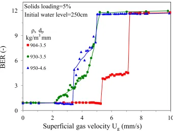
5.1 The effect of particle property on bed expansion ratio

Three different particles are employed to investigate the bed expansion ratio, including 904kg/m3, 3.5mm; 930kg/m3, 3.5mm and 950kg/m3, 4.6mm. The variations of bed expansion ratio as a function of superficial gas velocity for three different particles are shown in Fig 5.2. It is observed that the bed remains fixed until a certain gas flow rate (Ug1), subsequently increases with gas flow rate for different solid densities and initial

water level. Since at lower gas flow rate, drag force caused by the downward flow cannot balance the net buoyancy of the particles acting in the opposite direction. Therefore, the particles keep as the packed bed at the top of the column. With increasing the gas flow rate, a condition (downward drag force=upward net buoyancy) is obtained where the lowest position of the particles begin to fluidize. The velocity corresponding to the flow rate is referred as initial fluidization velocity (Ug1). With further increasing the gas flow

rate, more and more particles separate from the packed bed then fluidize, meanwhile, bed expansion ratio increases as drag force increases with increasing gas flow rate. When some particles reach the bottom of the bed, the velocity corresponding to this gas flow rate is termed as the full expansion velocity (Ug2). As the limit of the column height, the

bed expansion ratio keeps constant after the full expansion velocity. Furthermore, in three initial water levels (130cm, 190cm and 250cm), the patterns of the bed expansion ratio are like each other, which means the influence of the initial water level can be neglected.

In addition, P1 (904kg/m3) has the highest initial fluidization velocity and full expansion velocity as the difference between the density of P1 and liquid is the biggest among three particles. Also, P2 and P3 have almost same initial fluidization velocity and full

(54)

(a)

(b) 0

3 6 9 12

0 2 4 6 8 10

BE

R

(-)

Superficial gas velocity U

_g

(mm/s)

904-3.5

930-3.5

950-4.6

0 3 6 9 12

0 2 4 6 8 10

BE

R

(-)

Superficial gas velocity U

_g

(mm/s)

904-3.5

930-3.5

950-4.6

Solids loading=5% Initial water level=130cm

ρs dp

kg/m3 mm

ρs dp

kg/m3 mm

(55)

(c)

Figure 5.2 The variations of bed expansion ratio as a function of superficial gas velocity for three different particles: (a) 130cm, (b) 190cm and (c) 250cm.

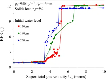
5.2 The effect of water level on bed expansion ratio

Three different particles are employed to investigate the effect of water level on bed expansion ratio, including 904kg/m3, 3.5mm; 930kg/m3, 3.5mm and 950kg/m3, 4.6mm. The variations of bed expansion ratio as a function of superficial gas velocity for three water levels with three different particles are shown in Fig 5.3. It is observed from the figure that the bed remains as fixed until a certain gas flow rate, which is termed as the initial fluidization velocity. Thus, with further increasing the gas flow rate, bed expansion increases as more and more particles begin to fluidize. After some of the particles reach the bottom, this gas flow rate corresponding to the gas velocity is referred as the full expansion velocity. When the gas flow rate is higher than the full expansion velocity, as the limit of the total column height, the bed expansion ratio remains constant. The particles have the same trends as the trend in Fig 5.2.

0 3 6 9 12

0 2 4 6 8 10

BE

R

(-)

Superficial gas velocity U

_g

(mm/s)

904-3.5

930-3.5

950-4.6 ρs dp

kg/m3 _mm

(56)

(57)

(a)

(b) 0

3 6 9 12

0 2 4 6 8 10

BE

R

(-)

Superficial gas velocity U

_g

(mm/s)

130cm

190cm

250cm

0 3 6 9 12

0 2 4 6 8 10

BE

R

(-)

Superficial gas velocity U

_g

(mm/s)

130cm

190cm

250cm

ρs=904kg/m3, dp=3.5mm

Solids loading=5%

Solids loading=5% Initial water level

(58)

(c)

Figure 5.3 The variations of bed expansion ratio as a function of superficial gas velocity for three water levels with three different particles: (a) 904kg/m3, (b)

930kg/m3 and (c) 950kg/m3.

5.3 The effect of solids loading on bed expansion ratio

P2 (930kg/m3) has been employed to investigate the effect of solids loading on bed expansion ratio. The variations of bed expansion ratio as a function of superficial gas velocity for three solids loadings are shown in Fig 5.4. It is observed from the figure that with increasing the gas flow rate to the initial fluidization velocity, the fixed bed begins to fluidize; because when the gas velocity reaches the initial fluidization velocity, the upward force equals to the downward force. With further increasing the gas flow rate, the bed expansion ratio increases as more and more particles keep in motion. Due to the limit of the total height of the column, the maximum bed expansion ratio is achieved. This gas flow rate is referred as the full expansion velocity.

0 3 6 9 12

0 2 4 6 8 10

BE

R

(-)

Superficial gas velocity U

_g

(mm/s)

130cm

190cm

250cm

Solids loading=5%

(59)

(a)

(b) 0

3 6 9 12

0 2 4 6 8 10

BE

R

(-)

Superficial gas velocity U

_g

(mm/s)

5%

10%

15%

0 3 6 9 12

0 2 4 6 8 10

BE

R

(-)

Superficial gas velocity U

_g

(mm/s)

5%

10%

15%

Initial water level =130cm

Initial water level =190cm Solids loading

(60)

(c)

Figure 5.4 The variations of bed expansion ratio as a function of superficial gas velocity for three solids loadings: (a) 130cm, (b) 190cm and (c) 250cm.

However, the limit of the column height is not an important parameter, to avoid the effect of column height limitation, bed expansion percentage should be used. The bed

expansion percentage is calculated as

Hbed H0

⎛

⎝

⎜ ⎞

⎠ ⎟

max

. The variations of bed expansion

percentage as a function of superficial gas velocity for three solids loadings are shown in Fig 5.5.

0 3 6 9 12

0 2 4 6 8 10

BE

R

(-)

Superficial gas velocity U

_g

(mm/s)

5%

10%

15%

(61)

(a) (b) 0 0.2 0.4 0.6 0.8 1

0 2 4 6 8 10

B

ed

expa

ns

ion

pe

rc

ent

age

(

%

)

Superficial gas velocity U

_g

(mm/s)

5% 10% 15% 0 0.2 0.4 0.6 0.8 1

0 2 4 6 8 10

B

ed

expa

ns

ion

pe

rc

ent

age

(

%

)

Superficial gas velocity U

_g

(mm/s)

5%

10%

15% ρs=930kg/m3, dp=3.5mm

Initial water level =190cm Solids loading

Bubble-Induced Inverse Gas-Liquid-Solid Fluidized Bed

Scholarship@Western

Scholarship@Western

Bubble-Induced Inverse Gas-Liquid-Solid Fluidized Bed

Bubble-Induced Inverse Gas-Liquid-Solid Fluidized Bed

Keywords

Acknowledgments

Table of Contents

List of Tables

List of Figures

List of Appendices

Chapter 1

1

General Introduction

1.1 Introduction

1.2 Objectives

1.3 Thesis structure

Chapter 2

2

Literature review

2.1 Introduction

2.2 Hydrodynamic characters in inverse fluidization

2.2.1

Flow regimes

2.2.2

Pressure gradient

(

)

(

)

2.2.3

Minimum fluidization velocity

2.2.4

Phase holdups

2.2.5

Bed expansion

2.2.6

Particle property

2.2.7

Bubble behaviors

2.2.8

Residence time distribution (RTD)

∑

∑

2.2.9

Mass transfer property

2.2.10 Heat transfer property

2.3 Hydrodynamic characters in bubble-induced inverse

three-phase fluidized bed

Chapter 3

3

Experimental apparatus and measurement methods

3.1 The structure of bubble-induced inverse gas-liquid-solid

fluidized bed

3.2 Experimental procedure

3.3 Measurement procedures

3.3.1

Measurement of superficial gas velocity

3.3.2

Measurement of pressure drop

3.3.3

Measurement of average phase holdups

3.3.4

Measurement of local phase holdups

3.4 Particle properties

ε

Chapter 4

4

Experimental investigation of flow regimes

4.1 Initial fluidization velocity (

U

)

U

(m

m

/s

)

Solids loading (%)

4.2 Full expansion velocity (

U