DIFFERENCE SCHEMES FOR NONLINEAR BVPs USING
RUNGE-KUTTA IVP-SOLVERS
I. P. GAVRILYUK, M. HERMANN, M. V. KUTNIV, AND V. L. MAKAROV
Received 11 November 2005; Revised 1 March 2006; Accepted 2 March 2006
Difference schemes for two-point boundary value problems for systems of first-order nonlinear ordinary differential equations are considered. It was shown in former papers of the authors that starting from the two-point exact difference scheme (EDS) one can de-rive a so-called truncated difference scheme (TDS) which a priori possesses an arbitrary given order of accuracyᏻ(|h|m) with respect to the maximal step size|h|. Thism-TDS represents a system of nonlinear algebraic equations for the approximate values of the exact solution on the grid. In the present paper, new efficient methods for the imple-mentation of anm-TDS are discussed. Examples are given which illustrate the theorems proved in this paper.
Copyright © 2006 I. P. Gavrilyuk et al. This is an open access article distributed under the Creative Commons Attribution License, which permits unrestricted use, distribution, and reproduction in any medium, provided the original work is properly cited.
1. Introduction
This paper deals with boundary value problems (BVPs) of the form
u(x) +A(x)u=f(x,u), x∈(0, 1), B0u(0) +B1u(1)=d, (1.1)
where
A(x),B0,B1,∈Rd×d, rankB0,B1=d, f(x,u),d,u(x)∈Rd, (1.2)
anduis an unknownd-dimensional vector-function. On an arbitrary closed irregular grid
ωh=xj: 0=x0< x1< x2<···< xN=1
, (1.3)
there exists a unique two-point exact difference scheme (EDS) such that its solution co-incides with a projection of the exact solution of the BVP onto the gridωh . Algorithmical realizations of the EDS are the so-called truncated difference schemes (TDSs). In [14] an algorithm was proposed by which for a given integerman associated TDS of the order of accuracym(or shortlym-TDS) can be developed.
The EDS and the corresponding three-point difference schemes of arbitrary order of accuracy m(so-called truncated difference schemes of rank mor shortlym-TDS) for BVPs for systems of second-order ordinary differential equations (ODEs) with piecewise continuous coefficients were constructed in [8–18,20,23,24]. These ideas were further developed in [14] where two-point EDS and TDS of an arbitrary given order of accuracy for problem (1.1) were proposed. One of the essential parts of the resulting algorithm was the computation of the fundamental matrix which influenced considerably its complex-ity. Another essential part was the use of a Cauchy problem solver (IVP-solver) on each subinterval [xj−1,xj] where a one-step Taylor series method of the ordermhas been cho-sen. This supposes the calculation of derivatives of the right-hand side which negatively influences the efficiency of the algorithm.
The aim of this paper is to remove these two drawbacks and, therefore, to improve the computational complexity and the effectiveness of TDS for problem (1.1). We pro-pose a new implementation of TDS with the following main features: (1) the complexity is significantly reduced due to the fact that no fundamental matrix must be computed; (2) the user can choose an arbitrary one-step method as the IVP-solver. In our tests we have considered the Taylor series method, Runge-Kutta methods, and the fixed point it-eration for the equivalent integral equation. The efficiency of 6th- and 10th-order ac-curate TDS is illustrated by numerical examples. The proposed algorithm can also be successfully applied to BVPs for systems of stiff ODEs without use of the “expensive” IVP-solvers.
Note that various modifications of the multiple shooting method are considered to be most efficient for problem (1.1) [2,3,6, 22]. The ideas of these methods are very close to that of EDS and TDS and are based on the successive solution of IVPs on small subintervals. Although there exist a priori estimates for all IVP-solver in use, to our best knowledge only a posteriori estimates for the shooting method are known.
The theoretical framework of this paper allows to carry out a rigorous mathematical analysis of the proposed algorithms including existence and uniqueness results for EDS and TDS, a priori estimates for TDS (see, e.g.,Theorem 4.2), and convergence results for an iterative procedure of its practical implementation.
The paper is organized as follows. InSection 2, leaning on [14], we discuss the proper-ties of the BVP under consideration including the existence and uniqueness of solutions.
Section 3deals with the two-point exact difference schemes and a result about the
2. The given BVP: existence and uniqueness of the solution
The linear part of the differential equation in (1.1) determines the fundamental matrix (or the evolution operator)U(x,ξ)∈Rd×d which satisfies the matrix initial value prob-lem (IVP)
∂U(x,ξ)
∂x +A(x)U(x,ξ)=0, 0≤ξ≤x≤1, U(ξ,ξ)=I, (2.1) whereI∈Rd×dis the identity matrix. The fundamental matrixUsatisfies the semigroup property
U(x,ξ)U(ξ,η)=U(x,η), (2.2)
and the inequality (see [14])
U(x,ξ)≤exp
c1(x−ξ). (2.3)
In what follows we denote byu ≡√uTuthe Euclidean norm ofu∈Rdand we will use the subordinate matrix norm generated by this vector norm. For vector-functions u(x)∈C[0, 1], we define the norm
u0,∞,[0,1]= max x∈[0,1]
u(x). (2.4)
Let us make the following assumptions.
(PI) The linear homogeneous problem corresponding to (1.1) possesses only the triv-ial solution.
(PII) For the elements of the matrixA(x)=[ai j(x)]id,j=1it holds thatai j(x)∈C[0, 1], i,j=1, 2,...,d.
The last condition implies the existence of a constantc1such that
A(x)≤c1 ∀x∈[0, 1]. (2.5)
It is easy to show that condition (PI) guarantees the nonsingularity of the matrixQ≡
B0+B1U(1, 0) (see, e.g., [14]).
Some sufficient conditions which guarantee that the linear homogeneous BVP corre-sponding to (1.1) has only the trivial solution are given in [14].
Let us introduce the vector-function
u(0)(x)≡U(x, 0)Q−1d (2.6)
(which exists due to assumption (PI) for allx∈[0, 1]) and the set
ΩD,β(·) ≡v(x)=vi(x) di=1,vi(x)∈C[0, 1],i=1, 2,...,d,
v(x)−u(0)(x)≤β(x), x∈D, (2.7)
Further, we assume the following assumption.
(PIII) The vector-functionf(x,u)= {fj(x,u)}dj=1satisfies the conditions
fj(x,u)∈C[0, 1]×Ω[0, 1],r(·) , f(x,u)≤K ∀x∈[0, 1],u∈Ω[0, 1],r(·) ,
f(x,u)−f(x,v)≤Lu−v ∀x∈[0, 1],u,v∈Ω
[0, 1],r(·) , r(x)≡Kexpc1x x+Hexp
c1 ,
(2.8)
whereH≡Q−1B1.
Now, we discuss sufficient conditions which guarantee the existence and uniqueness of a solution of problem (1.1). We will use these conditions below to prove the existence of the exact two-point difference scheme and to justify the schemes of an arbitrary given order of accuracy.
We begin with the following statement. Theorem2.1. Under assumptions (PI)–(PIII) and
q≡Lexpc1 1 +Hexp
c1 <1, (2.9)
problem (1.1) possesses in the setΩ([0, 1],r(·))a unique solutionu(x)which can be deter-mined by the iteration procedure
u(k)(x)= 1
0G(x,ξ)f
ξ,u(k−1)(ξ) dξ+u(0)(x), x∈[0, 1], (2.10)
with the error estimate
u(k)−u
0,∞,[0,1]≤ qk
1−qr(1), (2.11)
where
G(x,ξ)≡ ⎧ ⎨
⎩−−UU((xx, 0), 0)HUHU(1,(1,ξξ),) +U(x,ξ), 0ξ≤≤xx≤≤1ξ,. (2.12)
3. Existence of an exact two-point difference scheme
Let us consider the space of vector-functions (uj)Nj=0defined on the gridωh and equipped with the norm
u0,∞,ωh=0max≤j≤Nuj. (3.1)
Throughout the paperMdenotes a generic positive constant independent of|h|. Given (vj)Nj=0⊂Rdwe define the IVPs (each of the dimensiond)
dYjx,v j−1
dx +A(x)Yj
x,vj−1 =f
x,Yjx,v j−1
, x∈xj−1,xj
, Yjx
j−1,vj−1 =vj−1, j=1, 2,...,N.
The existence of a unique solution of (3.2) is postulated in the following lemma. Lemma3.1. Let assumptions (PI)–(PIII) be satisfied. If the grid vector-function(vj)Nj=0 be-longs toΩ(ωh ,r(·)), then the problem (3.2) has a unique solution.
Proof. The question about the existence and uniqueness of the solution to (3.2) is equiv-alent to the same question for the integral equation
Yjx,v
j−1 =
x,vj−1,Yj , (3.3)
where
x,vj−1,Yj ≡Ux,xj−1 vj−1+ x
xj−1
U(x,ξ)fξ,Yjξ,vj−1
dξ, x∈xj−1,xj.
(3.4)
We define thenth power of the operator(x,vj−1,Yj) by
nx,v
j−1,Yj = x,vj−1,n−1x,vj−1,Yj , n=2, 3,.... (3.5)
LetYj(x,v
j−1)∈Ω([xj−1,xj],r(·)) for (vj)Nj=0∈Ω(ωh ,r(·)). Then
x,vj−1,Yj −u(0)(x)
≤Ux,xj−1 vj−1−u(0)
xj−1 + x
xj−1
U(x,ξ)f
ξ,Yjξ,vj−1 dξ
≤Kexpc1x xj−1+Hexp
c1 +K
x−xj−1 exp
c1
x−xj−1
≤Kexpc1x x+Hexp
c1 =r(x), x∈
xj−1,xj
,
(3.6)
that is, for grid functions (vj)Nj=0∈Ω(ωh ,r(·)) the operator(x,vj−1,Yj) transforms the
setΩ([xj−1,xj],r(·)) into itself. Besides, forYj(x,v
j−1),Yj(x,vj−1)∈Ω([xj−1,xj],r(·)), we have the estimate
x,vj−1,Yj − x,vj−1,Yj
≤ x
xj−1
U(x,ξ)f
ξ,Yjξ,vj−1
−fξ,Yjξ,vj−1 dξ
≤Lexpc1hj x
xj−1
Yjξ,v
j−1 −Yjξ,vj−1 dξ
≤Lexpc1hj x−xj−1 Yj−Yj0,∞,[xj−1,xj].
Using this estimate, we get 2x,v
j−1,Yj − 2x,vj−1,Yj ≤Lexpc1hj
x
xj−1
x,vj−1,Yj − x,vj−1,Yj dξ
≤
Lexpc1hj x−xj−1 2
2! Y
j−Yj
0,∞,[xj−1,xj].
(3.8)
If we continue to determine such estimates, we get by induction
nx,v
j−1,Yj − nx,vj−1,Yj ≤
Lexpc1hj x−xj−1 n
n! Yj−Yj0,∞,[xj−1,xj]
(3.9)
and it follows that n·,v
j−1,Yj − n·,vj−1,Yj 0,∞,[xj−1,xj]≤
Lexpc1hj hj
n
n! Y
j−Yj
0,∞,[xj−1,xj].
(3.10)
Taking into account that [Lexp(c1hj)hj]n/(n!)→0 for n→ ∞, we can fix n large enough such that [Lexp(c1hj)hj]n/(n!)<1, which yields that thenth power of the oper-atorn(x,v
j−1,Yj) is a contractive mapping of the setΩ([xj−1,xj],r(·)) into itself. Thus (see, e.g., [1] or [25]), for (vj)N
j=0∈Ω(ωh,r(x)), problem (3.3) (or problem (3.2)) has a
unique solution.
We are now in the position to prove the main result of this section.
Theorem3.2. Let the assumptions ofTheorem 2.1be satisfied. Then, there exists a two-point EDS for problem (1.1). It is of the form
uj=Yj
xj,uj−1 , j=1, 2,...,N, (3.11)
B0u0+B1uN=d. (3.12)
Proof. It is easy to see that
d dxYj
x,uj−1 +A(x)Yj
x,uj−1 =f
x,Yjx,u j−1
, x∈xj−1,xj,
Yjx
j−1,uj−1 =uj−1, j=1, 2,...,N.
(3.13)
Due toLemma 3.1the solvability of the last problem is equivalent to the solvability of problem (1.1). Thus, the solution of problem (1.1) can be represented by
u(x)=Yjx,u
j−1 , x∈
xj−1,xj, j=1, 2,...,N. (3.14)
For the further investigation of the two-point EDS, we need the following lemma. Lemma3.3. Let the assumptions ofLemma 3.1be satisfied. Then, for two grid functions (uj)N
j=0and(vj)Nj=0inΩ(ωh,r(·)),
Yjx,u
j−1 −Yjx,vj−1 −Ux,xj−1 uj−1−vj−1
≤Lx−xj−1 exp
c1x−xj−1 +L x
xj−1
expc1(x−ξ)dξuj−1−vj−1. (3.15)
Proof. When proving Lemma 3.1, it was shown that Yj(x,u
j−1), Yj(x,vj−1) belong to Ω([xj−1,xj],r(·)). Therefore it follows from (3.2) that
Yjx,u
j−1 −Yj
x,vj−1 −U
x,xj−1 uj−1−vj−1
≤L
x
xj−1
expc1(x−ξ)expc1ξ−xj−1 uj−1−vj−1
+Yjξ,u j−1 −Yj
ξ,vj−1 −U
ξ,xj−1 uj−1−vj−1 dξ
=Lexpc1
x−xj−1 x−xj−1 uj−1−vj−1
+L
x
xj−1
expc1(x−ξ)Yjξ,uj−1 −Yj
ξ,vj−1 −U
ξ,xj−1 uj−1−vj−1 dξ. (3.16)
Now, Gronwall’s lemma implies (3.15).
We can now prove the uniqueness of the solution of the two-point EDS (3.11)-(3.12). Theorem3.4. Let the assumptions ofTheorem 2.1be satisfied. Then there exists anh0>0 such that for|h| ≤h0the two-point EDS (3.11)-(3.12) possesses a unique solution(uj)Nj=0= (u(xj))Nj=0∈Ω(ωh ,r(·))which can be determined by the modified fixed point iteration
u(jk)−Uxj,xj−1 u(jk−)1=Yj
xj,u(jk−−11) −U
xj,xj−1 u(jk−−11), j=1, 2,...,N,
B0u(0k)+B1uN(k)=d, k=1, 2,...,
u(0)j =Uxj, 0 Q−1d, j=0, 1,...,N.
(3.17)
The corresponding error estimate is
u(k)−u 0,∞,ωh≤
qk 1
1−q1r(1), (3.18)
Proof. Taking into account (2.2), we apply successively the formula (3.11) and get
Substituting (3.19) into the boundary condition (3.12), we obtain
Let (vj)Nj=0∈Ω(ωh ,r(·)), then we have (see the proof ofLemma 3.1)
Lemma 3.3and the estimate G(x,ξ)≤⎧⎨ ⎩
expc1(1 +x−ξ)H, 0≤x≤ξ, expc1(x−ξ)1 +Hexpc1 , ξ≤x≤1,
(3.27)
which has been proved in [14], the relation (3.22) implies which can be determined by the modified fixed point iteration (3.17) with the error
esti-mate (3.18).
4. Implementation of two-point EDS
wheremis a positive integer,Y(m)j(x
j,y(jm−)1) is the numerical solution of the IVP (3.2) on the interval [xj−1,xj] which has been obtained by some one-step method of the orderm (e.g., by the Taylor expansion or a Runge-Kutta method):
Y(m)jx
j,y(jm−1) =y (m) j−1+hjΦ
xj−1,y(jm−)1,hj , (4.3)
that is, it holds that
Y(m)jx
j,uj−1 −Yj
xj,uj−1 ≤Mhmj+1, (4.4) where the increment function (see, e.g., [6])Φ(x,u,h) satisfies the consistency condition Φ(x,u, 0)=f(x,u)−A(x)u. (4.5)
For example, in case of the Taylor expansion we have
Φxj−1,y(jm−1),hj =f
xj−1,y(jm−)1 −A
xj−1 y(jm−)1+ m
p=2 hpj−1
p!
dpYjx,y(m) j−1 dxp
x=xj−1
, (4.6)
and in case of an explicits-stage Runge-Kutta method we have Φxj−1,y(jm−)1,hj =b1k1+b2k2+···+bsks,
k1=fxj−1,y(jm−1) −A
xj−1 y(jm−)1, k2=fxj−1+c2hj,y(jm−1)+hja21k1 −A
xj−1+c2hj y(jm−1)+hja21k1 , ..
. ks=f
xj−1+cshj,y(jm−)1+hj
as1k1+as2k2+···+as,s−1ks−1
−Axj−1+cshj y(jm−)1+hj
as1k1+as2k2+···+as,s−1ks−1 ,
(4.7)
with the corresponding real parameters ci, ai j, i=2, 3,...,s, j=1, 2,...,s−1, bi, i=
1, 2,...,s.
In order to prove the existence and uniqueness of a solution of them-TDS (4.1)-(4.2) and to investigate its accuracy, the next assertion is needed.
Lemma4.1. Let the method (4.3) be of the order of accuracym. Moreover, assume that the increment functionΦ(x,u,h)is sufficiently smooth, the entriesaps(x)of the matrixA(x) belong toCm[0, 1], and there exists a real numberΔ>0such that fp(x,u)∈Ck,m−k([0, 1]×
Ω([0, 1],r(·) +Δ)), withk=0, 1,...,m−1andp=1, 2,...,d. Then
U(1)
xj,xj−1 −U
xj,xj−1 ≤Mh2j, (4.8)
h1
j
Y(m)jxj,vj−1 −U(1)
xj,xj−1 vj−1≤K+Mhj, (4.9)
hj1Y(m)jxj,u
j−1 −Y(m)j
xj,vj−1 −U(1)
xj,xj−1 uj−1−vj−1
≤L+Mhj uj−1−vj−1,
where(uj)Nj=0, (vj)Nj=0∈Ω(ωh ,r(·) +Δ). The matrixU(1)(xj,xj−1)is defined by
U(1)xj,xj
−1 =I−hjAxj−1 . (4.11)
Proof. Insertingx=xjinto the Taylor expansion of the functionU(x,xj−1) at the point
xj−1gives
Uxj,xj−1 =U(1)
xj,xj−1 + xj
xj−1
xj−t d 2Ut,xj
−1
dt2 dt. (4.12)
From this equation the inequality (4.8) follows immediately. It is easy to verify the following equalities:
1 hj
Y(m)jxj,v
j−1 −U(1)
xj,xj−1 vj−1
=Φxj−1,vj−1,hj +A
xj−1 vj−1
=Φxj−1,vj−1, 0 +hj∂Φ
xj−1,vj−1, ¯h
∂h +A
xj−1 vj−1
=fxj−1,vj−1 +hj∂Φ
xj−1,vj−1, ¯h
∂h ,
1 hj
Y(m)jx
j,uj−1 −Y(m)jxj,vj−1 −U(1)xj,xj−1 uj−1−vj−1
=Φxj−1,uj−1,hj −Φxj−1,vj−1,hj +Axj−1 uj−1−vj−1
=fxj−1,uj−1 −f
xj−1,vj−1 +hj
∂Φxj−1,uj−1, ¯h
∂h −
∂Φxj−1,vj−1, ¯h
∂h
=fxj−1,uj−1 −f
xj−1,vj−1
+hj
1
0 ∂2Φx
j−1,θuj−1+ (1−θ)vj−1, ¯h
∂h∂u dθ·
uj−1−vj−1 ,
(4.13)
where ¯h∈(0,|h|), which imply (4.9)-(4.10). The proof is complete. Now, we are in the position to prove the main result of this paper.
solution which can be determined by the modified fixed point iteration
The corresponding error estimate is
y(m,n)−u
Proof. From (4.1) we deduce successively
y(1m)=U(1)
SubstitutingyN(m)into the boundary conditions (4.2), we get
Let us show that the matrix in square brackets is regular. Here and in the following we
which can be easily derived using the estimate (4.8). We have
forh0small enough. Here we have used the inequality
Estimates (4.18) and (4.23) imply
Now we use Banach’s fixed point theorem. First of all we show that the operator
(m) (4.1)-(4.2) has a unique solution which can be determined by the modified fixed point iteration (4.14) with the error estimate
The errorz(jm)=yj(m)−ujof the solution of scheme (4.1)-(4.2) satisfies
z(jm)−U(1)x
j,xj−1 z(jm−)1=ψ(m)
xj,y(jm−1) , j=1, 2,...,N,
B0z(0m)+B1z (m) N =0,
(4.32)
where the residuum (the approximation error)ψ(m)(x
j,y(jm−)1) is given by
ψ(m)x
j,y(jm−)1 =
Y(m)jxj,uxj− 1
−Yjxj,uxj− 1
+Y(m)jxj,yj(m−)1 −Y(m)j
xj,u
xj−1
−U(1)x
j,xj−1 y(jm−)1−u
xj−1
. (4.33)
We rewrite problem (4.32) in the equivalent form
z(jm)=
N
i=1
G(1)h xj,xi ψ(m)
xi,yi(−m1) . (4.34)
Then (4.28) andLemma 4.1imply
z(m) j ≤
expc1 1 +Hexp
c1
+M|h|
N
i=1 ψ(m)
xi,y(i−m1)
≤expc1 1 +Hexp
c1
+M|h|
×
M|h|m+N i=1 hi
L+hiM z(i−m1)
≤q2z(m)0,∞,ωh+M|h|
m.
(4.35)
The last inequality yields
z(m)
0,∞,ωh≤M|h|
m. (4.36)
Now, from (4.31) and (4.36) we get the error estimate for the method (4.15): y(m,n)−u
0,∞,ωh≤y
(m,n)−y(m)
0,∞,ωh+y
(m)−u
0,∞,ωh≤M
qn
2+|h|m , (4.37)
which completes the proof.
Above we have shown that the nonlinear system of equations which represents the TDS can be solved by the modified fixed point iteration. But actually Newton’s method is used due to its higher convergence rate. The Newton method applied to the system (4.1)-(4.2) has the form
y(jm,n)−∂Y
(m)jx
j,y(jm−1,n−1)
∂u y
(m,n) j−1 =Y(m)j
xj,y(jm−1,n−1) −y (m,n−1)
j−1 , j=1, 2,...,N, B0y(0m,n)+B1y(Nm,n)=0, n=1, 2,...,
y(jm,n)=y(jm,n−1)+yj(m,n), j=0, 1,...,N,n=1, 2,...,
(4.38)
where
∂Y(m)jx j,y(jm−)1
∂u =I+hj
∂Φxj−1,y(jm−)1,hj ∂u
=I+hj
∂fxj−1,y(jm−)1
∂u −A
xj−1
+Oh2j
(4.39)
and∂f(xj−1,y(jm−1))/∂uis the Jacobian of the vector-functionf(x,u) at the point (xj−1,y(jm−1)). Denoting
Sj=∂Y
(m)jx
j,y(jm−1,n−1)
∂u , (4.40)
the system (4.38) can be written in the following equivalent form:
B0+B1S
y0(m,n)= −B1ϕ, y (m,n) 0 =y
(m,n−1) 0 +y
(m,n)
0 , (4.41)
where
S=SNSN−1···S1, ϕ=ϕN, ϕ0=0, ϕj=Sjϕj−1+Y(m)j
xj,y(jm−1,n−1) −y (m,n−1)
j−1 , j=1, 2,...,N.
(4.42)
After solving system (4.41) with a (d×d)-matrix (this requiresᏻ(N) arithmetical op-erations since the dimensiondis very small in comparison withN) the solution of the system (4.38) is then computed by
y(jm,n)=SjSj−1···S1y0(m,n)+ϕj,
When using Newton’s method or a quasi-Newton method, the problem of choosing an appropriate start approachy(jm,0), j=1, 2,...,N, arises. If the original problem contains a natural parameter and for some values of this parameter the solution is known or can be easily obtained, then one can try to continue the solution along this parameter (see, e.g., [2, pages 344–353]). Thus, let us suppose that our problem can be written in the generic form
u(x) +A(x)u=g(x,u,λ), x∈(0, 1), B0u(0) +B1u(1)=d, (4.44)
whereλdenotes the problem parameter. We assume that for eachλ∈[λ0,λk] an isolated solutionu(x,λ) exists and depends smoothly onλ.
If the problem does not contain a natural parameter, then we can introduce such a parameterλartificially by forming the homotopy function
g(x,u,λ)=λf(x,u) + (1−λ)f1(x), (4.45)
with a given functionf1(x) such that the problem (4.46) has a unique solution. Now, forλ=0 the problem (4.44) is reduced to the linear BVP
u(x) +A(x)u=f1(x), x∈(0, 1), B0u(0) +B1u(1)=d, (4.46)
while forλ=1 we obtain our original problem (1.1). Them-TDS for the problem (4.44) is of the form
y(jm)(λ)=Y(m)jx
j,y(jm−)1,λ , j=1, 2,...,N,
B0y(0m)(λ) +B1y (m) N (λ)=d.
(4.47)
The differentiation byλyields the BVP
dy(jm)(λ)
dλ =
∂Y(m)jx j,y(jm−)1,λ
∂λ +
∂Y(m)jx j,y(jm−)1,λ
∂u
dy(jm)(λ)
dλ , j=1, 2,...,N,
B0dy (m) 0 (λ)
dλ +B1
dy(Nm)(λ) dλ =0,
(4.48)
which can be further reduced to the following system of linear algebraic equations for the unknown functionv0(m)(λ)=dy(0m)(λ)/dλ:
B0+B1S
where
S=SNSN−1···S1, Sj=
∂Y(m)jx j,y(jm−)1,λ
∂u , j=1, 2,...,N,
ϕ=ϕN, ϕ0 =0, ϕj=Sjϕj−1+
∂Y(m)jxj,y(m) j−1,λ
∂λ , j=1, 2,...,N.
(4.50)
Moreover, forv(jm)(λ)=dy(jm)(λ)/dλwe have the formulas
v(jm)(λ)=SjSj−1···S1v(0m)+ϕj, j=1, 2,...,N. (4.51)
The start approach for Newton’s method can now be obtained by
y(jm,0)(λ+λ)=y(jm)(λ) +λv(jm)(λ), j=0, 1,...,N. (4.52)
Example 4.4. This BVP goes back to Troesch (see, e.g., [26]) and represents a well-known test problem for numerical software (see, e.g., [5, pages 17-18]):
u=λsinh(λu), x∈(0, 1), λ >0, u(0)=0, u(1)=1. (4.53)
We apply the truncated difference scheme of orderm:
y(jm)=Y(m)jxj,y(jm−1) , j=1, 2,...,N,
B0y(0m)+B1y (m) N =d,
(4.54)
where the following Taylor series IVP-solver is used:
Y(m)jxj,y(m) j−1 =y
(m) j−1+hjF
xj−1,y(jm−)1 + m
p=2 hpj
p!
dpYjx,y(m) j−1 dxp
x=xj−1 ,
y(jm)= ⎛ ⎝y
(m) 1,j y(2,mj)
⎞
⎠, A=
# 0 −1
0 0
$
, B0=
#
1 0
0 0
$
, B1=
#
0 0
1 0
$ ,
d= #
0 1 $
, F(x,u)= −Au+f(x,u)= #
−u2 λsinhλu1
$
.
Let us describe the algorithm for the computation ofY(m)j(x x=xj−1. This function satisfies the IVP
d2Yj
Substituting this series into the differential equation (4.57), we get
Y1,i+2= λRi
Performing the simple transformations
r=coshpp=ps, s=sinhpp=pr (4.61)
and applying formula (8.20b) from [4], we arrive at the recurrence equations
Ri=1
The corresponding initial conditions are
The Jacobian is given by
j−1)/∂ulsatisfy the differential equations
d2Y
for the computation ofY1,p,ul, we get the recurrence algorithm
where
Y1,p,λ= ∂Y1,p
xj,y(jm−)1,λ
∂λ . (4.69)
Taking into account that Y1,jλ(xj,y(jm−)1,λ)=∂Y1j(xj,y(j−m)1,λ)/∂λ satisfies the differential equation
d2Yj 1,λ dx2 =λ
2cosh
p(x) Y1,jλ+ sinh
p(x) +p(x) coshp(x) , (4.70)
we obtain forY1,p,λthe recurrence relation
Y1,i+2,λ=( 1 i+ 1)(i+ 2)
λ2 i
k=2
Y1,k,λSi−k+Ri+ i
k=0 PkSi−k
, i=2, 3,...,
Y1,2,λ=R0+2P0S0, Y1,3,λ=R1+P0S61+P1S0.
(4.71)
Taking into account the behavior of the solution we choose the grid
ωh=
xj=
exp(jα/N)−1
exp(α)−1 , j=0, 1, 2,...,N
, (4.72)
withα <0 which becomes dense forx→1. The step sizes of this grid are given byh1=x1 andhj+1=hjexp(α/N),j=1, 2,...,N−1. Note that the use of the formulahj=xj−xj−1,
j=1, 2,...,N, forj→Nand|α|large enough (α= −26) implies a large absolute roundoff error since some ofxj,xj−1lie very close together.
The a posteriori Runge estimator was used to arrive at the right boundary with a given toleranceε: the tolerance was assumed to be achieved if the following inequality is ful-filled:
max ⎧ ⎨ ⎩
y
(m) N −y
(m) 2N maxy(2mN), 10−5
0,∞,ωh
, dy (m)
N /dx−dy (m) 2N/dx maxdy(2mN)/dx, 10−5
0,∞,ωh
⎫ ⎬
⎭≤2m−1 ε. (4.73)
(a system of nonlinear algebraic equations) was solved by Newton’s method with the stopping criterion
max ⎧ ⎨ ⎩
y
(m,n)−y(m,n−1) maxy(m,n), 10−5
0,∞,ωh
,dy
(m,n)/dx−dy(m,n−1)/dx maxdy(m,n)/dx, 10−5
0,∞,ωh
⎫ ⎬ ⎭≤0.5ε,
(4.74)
wheren=1, 2,..., 10 denotes the iteration number. Setting the value of the unknown first derivative at the pointx=0 equal tosthe solution of Troesch’s test problem can be represented in the form (see, e.g., [22])
u(x,s)=2 λarcsinh
)
s·sn(λx,k) 2·cn(λx,k) *
, k2=1−s2
4, (4.75)
where sn(λx,k), cn(λx,k) are the elliptic Jacobi functions and the parameterssatisfies the equation
2 λarcsinh
)
s·sn(λ,k) 2·cn(λ,k) *
=1. (4.76)
For example, for the parameter valueλ=5 one getss=0.457504614063·10−1, and for λ=10 it holds thats=0.35833778463·10−3. Using the homotopy method (4.52) we have computed numerical solutions of Troesch’s problem (4.53) forλ∈[1, 62] using a step-size λ. The numerical results forλ=10, 20, 30, 40, 45, 50, 61 computed with the difference scheme of the order of accuracy 7 on the grid (4.72) withα= −26 are given in
Table 4.1, where CPU∗is the time needed by the processor in order to solve the sequence of Troesch problems beginning withλ=1 and using the stepλuntil the value ofλgiven in the table is reached. The numerical results forλ=61, 62 computed with the difference scheme of the order of accuracy 10 on the grid withα= −26 are given inTable 4.2. The real deviation from the exact solution is given by
Error=max ⎧ ⎨ ⎩
y
(m)−u maxy(m), 10−5
0,∞,ωh
, dy
(m)/dx−du/dx maxdy(m)/dx, 10−5
0,∞,ωh
⎫ ⎬ ⎭.
(4.77)
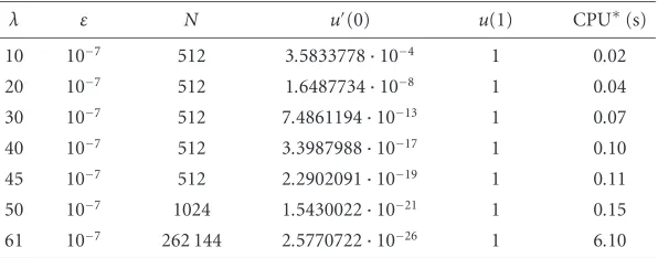
Table 4.1. Numerical results for the TDS withm=7 (λ=4).
λ ε N u(0) u(1) CPU∗(s)
10 10−7 512 3.5833778·10−4 1 0.02
20 10−7 512 1.6487734·10−8 1 0.04
30 10−7 512 7.4861194·10−13 1 0.07
40 10−7 512 3.3987988·10−17 1 0.10
45 10−7 512 2.2902091·10−19 1 0.11
50 10−7 1024 1.5430022·10−21 1 0.15
61 10−7 262 144 2.5770722·10−26 1 6.10
Table 4.2. Numerical results for the TDS withm=10 (λ=2).
λ ε N Error CPU∗(s)
61 10−6 65 536 0.860·10−5 3.50
61 10−8 131 072 0.319·10−7 7.17
62 10−6 262 144 0.232·10−5 8.01
62 10−8 262 144 0.675·10−8 15.32
Table 4.3. Numerical results for the code RWPM.
λ m it NFUN u(0) u(1) CPU (s)
10 11 9 12 641 3.5833779·10−4 1.000 0000 0.01
20 11 13 34 425 1.6487732·10−8 0.999 9997 0.02
30 14 16 78 798 7.4860938·10−13 1.000 0008 0.05
40 15 24 172 505 3.3986834·10−17 0.999 9996 0.14
45 12 31 530 085 2.2900149·10−19 1.000 0003 0.30
To compare the results we have solved problem (4.53) with the multiple shooting code RWPM (see, e.g., [7] or [27]). For the parameter valuesλ=10, 20, 30, 40 the numerical IVP-solver used was the code RKEX78, an implementation of the Dormand-Prince em-bedded Runge-Kutta method 7(8), whereas forλ=45 we have used the code BGSEXP, an implementation of the well-known Bulirsch-Stoer-Gragg extrapolation method. In
Example 4.5. Let us consider the BVP for a system of stiffdifferential equations (see [21])
In order to solve this problem numerically we apply the TDS of the order of accuracy 6 given by
Runge-Kutta method of the order 6 (see, e.g., [6]):
Table 4.4. Numerical results for the TDS withm=6 (λ=100).
ε NFUN CPU
10−4 24 500 0.01
10−6 41 440 0.02
10−8 77 140 0.04
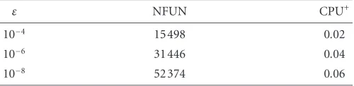
Table 4.5. Numerical results for the code RWPM (λ=100).
ε NFUN CPU+
10−4 15 498 0.02
10−6 31 446 0.04
10−8 52 374 0.06
Numerical results on the uniform grid
¯ ωh=
xj=jh, j=0, 1,...,N,h=N1
(4.82)
obtained by the TDS (4.79)–(4.81) are given inTable 4.4.
This problem was also solved by the code RWPM with the semi-implicit extrapolation method SIMPR as the IVP-solver within the multiple shooting method. As the start iter-ation we used the solution of the problem withλ=0. The numerical results are given in
Table 4.5, where CPU+denotes the aggregate time of the solution of the linear problem withλ=0 and of the problem withλ=100.
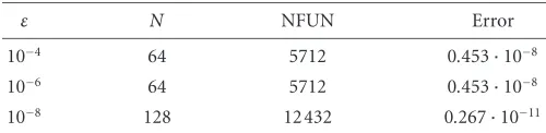
Example 4.6. Let us consider the periodic BVP (see [19])
u= −0.05u−0.02u2sinx+ 0.00005 sinxcos2x−0.05 cosx−0.0025 sinx, x∈(0, 2π), u(0)=u(2π), u(0)=u(2π),
(4.83)
which has the exact solutionu(x)=0.05 cosx. Numerical results on the uniform grid
¯ ωh=
xj=jh, j=0, 1,...,N,h=2Nπ
(4.84)
obtained by the TDS (4.79)–(4.81) with
y(jm)= ⎛ ⎝y
(m) 1,j y(2,mj)
⎞
⎠, B0=
#
1 0
0 1
$
, B1=
#
−1 0
0 −1 $
, d=
# 0 0 $
,
F(x,u)= ⎛
⎝ −u2
−0.05u2+ cosx + sinx0.00005 cos2x−0.02u21−0.0025 ⎞ ⎠
Table 4.6. Numerical results for the TDS withm=6.
ε N NFUN Error
10−4 64 5712 0.453·10−8
10−6 64 5712 0.453·10−8
10−8 128 12 432 0.267·10−11
are given inTable 4.6.
5. Conclusions
The main result of this paper is a new theoretical framework for the construction of dif-ference schemes of an arbitrarily given order of accuracy for nonlinear two-point bound-ary value problems. The algorithmical aspects of these schemes and their implementa-tion are only sketched and will be discussed in detail in forthcoming papers. Note that the proposed framework enables an automatic grid generation on the basis of efficient a posteriori error estimations as it is known from the numerical codes for IVPs. More precisely,Theorem 4.2asserts that if the coefficients of the TDS are computed by two embedded Runge-Kutta methods of the ordersmandm+ 1, then the corresponding dif-ference schemes for the given BVP are of the ordermandm+ 1, respectively. Thus, the difference between these two numerical solutions represents an a posteriori estimate of the local error of them-TDS (analogously to IVP-solvers) which can be used for an auto-matic and local grid refinement.
Acknowledgments
The authors would like to acknowledge the support which is provided by the Deutsche Forschungsgemeinschaft (DFG). Moreover, they thank the referees for their valuable re-marks which have improved the presentation.
References
[1] R. P. Agarwal, M. Meehan, and D. O’Regan,Fixed Point Theory and Applications, Cambridge Tracts in Mathematics, vol. 141, Cambridge University Press, Cambridge, 2001.
[2] U. M. Ascher, R. M. M. Mattheij, and R. D. Russell,Numerical Solution of Boundary Value Prob-lems for Ordinary Differential Equations, Prentice Hall Series in Computational Mathematics, Prentice Hall, New Jersey, 1988.
[3] P. Deuflhard and G. Bader,Multiple shooting techniques revisited, Numerical Treatment of Inverse Problems in Differential and Integral Equations (P. Deuflhard and E. Hairer, eds.), Birkh¨auser, Massachusetts, 1983, pp. 74–94.
[4] E. Hairer, S. P. Nørsett, and G. Wanner,Solving Ordinary Differential Equations. I. Nonstiff Prob-lems, 2nd ed., Springer Series in Computational Mathematics, vol. 8, Springer, Berlin, 1993. [5] M. Hermann (ed.),Numerische Behandlung von Differentialgleichungen. III,
Friedrich-Schiller-Universit¨at, Jena, 1985.
[6] M. Hermann,Numerik gew¨ohnlicher Differentialgleichungen, Oldenbourg, M¨unchen, 2004. [7] M. Hermann and D. Kaiser,RWPM: a software package of shooting methods for nonlinear
[8] M. V. Kutniv,Accurate three-point difference schemes for second-order monotone ordinary diff eren-tial equations and their implementation, Computational Mathematics and Mathematical Physics
40(2000), no. 3, 368–382, translated from Zhurnal Vychislitel’noi Matematiki i Matematich-eskoi Fiziki40(2000), no. 3, 387–401.
[9] ,Three-point difference schemes of a high order of accuracy for systems of second-order non-linear ordinary differential equations, Computational Mathematics and Mathematical Physics41
(2001), no. 6, 860–873, translated from Zhurnal Vychislitel’noi Matematiki i Matematicheskoi Fiziki41(2001), no. 6, 909–921.
[10] ,High-order accurate three-point difference schemes for systems of second-order ordinary differential equations with a monotone operator, Computational Mathematics and Mathematical Physics42(2002), no. 5, 754–738, translated from Zhurnal Vychislitel’noi Matematiki i Matem-aticheskoi Fiziki42(2002)), no. 5, 754–768.
[11] ,Three-point difference schemes of high accuracy order for systems of nonlinear second order ordinary differential equations with the boundary conditions of the third art, Visnyk Lvivskogo Universytetu, Seria Prykladna Mathematyka ta Informatyka4(2002), 61–66 (Ukrainian). [12] ,Modified three-point difference schemes of high-accuracy order for second order nonlinear
ordinary differential equations, Computational Methods in Applied Mathematics3(2003), no. 2, 287–312.
[13] M. V. Kutniv, V. L. Makarov, and A. A. Samarski˘ı,Accurate three-point difference schemes for second-order nonlinear ordinary differential equations and their implementation, Computational Mathematics and Mathematical Physics39(1999), no. 1, 40–55, translated from Zhurnal Vy-chislitel’noi Matematiki i Matematicheskoi Fiziki39(1999), no. 1, 45–60.
[14] V. L. Makarov, I. P. Gavrilyuk, M. V. Kutniv, and M. Hermann,A two-point difference scheme of an arbitrary order of accuracy for BVPs for systems of first order nonlinear ODEs, Computational Methods in Applied Mathematics4(2004), no. 4, 464–493.
[15] V. L. Makarov and V. V. Guminski˘ı,A three-point difference scheme of a high order of accuracy for a system of second-order ordinary differential equations (the nonselfadjoint case), Differentsial’nye Uravneniya30(1994), no. 3, 493–502, 550 (Russian).
[16] V. L. Makarov, I. L. Makarov, and V. G. Prikazˇcikov,Tochnye raznostnye shemy i shemy liubogo poriadka tochnosti dlia sistem obyknovennyh differencialnych uravnenij vtorogo poriadka, Diff er-entsial’nye Uravneniya15(1979), 1194–1205.
[17] V. L. Makarov and A. A. Samarski˘ı,Exact three-point difference schemes for second-order nonlinear ordinary differential equations and their realization, Doklady Akademii Nauk SSSR312(1990), no. 4, 795–800.
[18] ,Realization of exact three-point difference schemes for second-order ordinary differential equations with piecewise smooth coefficients, Doklady Akademii Nauk SSSR312(1990), no. 3, 538–543.
[19] M. Ronto and A. M. Samoilenko,Numerical-Analytic Methods in the Theory of Boundary-Value Problems, World Scientific, New Jersey, 2000.
[20] A. A. Samarski˘ı and V. L. Makarov,Realization of exact three-point difference schemes for second-order ordinary differential equations with piecewise-smooth coefficients, Differentsial’nye Urav-neniya26(1990), no. 7, 1254–1265, 1287.
[21] M. R. Scott and H. A. Watts,A systematized collection of codes for solving two-point boundary value problems, Numerical Methods for Differential Systems (A. K. Aziz, ed.), Academic Press, New York, 1976, pp. 197–227.
[22] J. Stoer and R. Bulirsch,Introduction to Numerical Analysis, Texts in Applied Mathematics, vol. 12, Springer, New York, 2002.
[24] ,Homogeneous difference schemes of a high order of accuracy on non-uniform nets, ˇZurnal Vyˇcislitel’ no˘ı Matematiki i Matematiˇcesko˘ı Fiziki1(1961), 425–440 (Russian).
[25] V. A. Trenogin,Functional Analysis, “Nauka”, Moscow, 1980.
[26] B. A. Troesch,A simple approach to a sensitive two-point boundary value problem, Journal of Computational Physics21(1976), no. 3, 279–290.
[27] W. Wallisch and M. Hermann,Schießverfahren zur L¨osung von Rand- und Eigenwertaufgaben, Teubner-Texte zur Mathematik, vol. 75, BSB B. G. Teubner, Leipzig, 1985.
I. P. Gavrilyuk: Berufsakademie Th¨uringen, Staatliche Studienakademie, Am Wartenberg 2, 99817 Eisenach, Germany
E-mail address:[email protected]
M. Hermann: Institute of Applied Mathematics, Friedrich Schiller University, Ernst-Abbe-Platz 1-4, 07740 Jena, Germany
E-mail address:[email protected]
M. V. Kutniv: Lviv Polytechnic National University, 12 St. Bandery Street, 79013 Lviv, Ukraine E-mail address:[email protected]
V. L. Makarov: Department of Numerical Analysis, Institute of Mathematics, National Academy of Sciences of Ukraine, 3 Tereshchenkivs’ka Street, 01601 Kyiv-4, Ukraine