Earth Planets Space,61, 825–833, 2009
Soft computing methods for geoidal height transformation
O. Akyilmaz, M. T. ¨Ozl¨udemir, T. Ayan, and R. N. C¸ elik
Istanbul Technical University, Faculty of Civil Engineering, Division of Geodesy, 34469 Maslak, Istanbul, Turkey
(Received June 18, 2008; Revised December 2, 2008; Accepted January 6, 2009; Online published August 31, 2009)
Soft computing techniques, such as fuzzy logic and artificial neural network (ANN) approaches, have enabled researchers to create precise models for use in many scientific and engineering applications. Applications that can be employed in geodetic studies include the estimation of earth rotation parameters and the determination of mean sea level changes. Another important field of geodesy in which these computing techniques can be applied is geoidal height transformation. We report here our use of a conventional polynomial model, the Adaptive Network-based Fuzzy (or in some publications, Adaptive Neuro-Fuzzy) Inference System (ANFIS), an ANN and a modified ANN approach to approximate geoid heights. These approximation models have been tested on a number of test points. The results obtained through the transformation processes from ellipsoidal heights into local levelling heights have also been compared.
Key words:Fuzzy inference systems, neural network, geoid undulation.
1.
Introduction
Height determination is one of the important tasks of sur-veying and geodesy. Satellite-based positioning techniques provide ellipsoidal heights. However, most users desire heights in a natural system rather than purely geometric el-lipsoidal heights. The most common natural system is or-thometric datum, which has a physical context and depends on Earth’s gravity field and, as such, refers to the geoid. The relation between ellipsoidal heights and orthometric heights can be established by geoid determination.
The most common method currently employed for pre-cise geoid determination is the gravimetric method. How-ever, the application of this technique is mainly dependent on the availability of high-resolution gravity data. In ad-dition, the terrestrial gravity networks usually follow the road network and do not cover the high mountains where the geoid heights change significantly. In the absence of ad-equate gravity data, the geoid can be modelled using other geometric methods, such as the astro-geodetic method or geoid height from GPS in conjunction with spirit levelling (Kuharet al., 2001). However, in most of the GPS appli-cations, users need to transform ellipsoidal heights into or-thometric heights in order to make them compatible with the existing orthometric heights on the local vertical datum (Engeliset al., 1985; Seeber, 2003).
The orthometric height is the distance of a point above the geoid measured along the plumb line through the point. The ellipsoidal height is calculated along the ellipsoidal normal, from the surface of any reference ellipsoid to the point of interest. The geoid height or geoid-ellipsoid sepa-ration is calculated along the ellipsoidal normal, from the
Copyright cThe Society of Geomagnetism and Earth, Planetary and Space Sci-ences (SGEPSS); The Seismological Society of Japan; The Volcanological Society of Japan; The Geodetic Society of Japan; The Japanese Society for Planetary Sci-ences; TERRAPUB.
surface of any reference ellipsoid to the geoid. There-fore, an essential requirement of any transformation of el-lipsoidal heights to orthometric heights is that the geoid height must refer to the same reference ellipsoid (Feather-stone, 2001).
From the above definitions, the geoid height at each point can be given as follows,
ξ ≈h−H (1)
where ξ is either the geoidal undulation or the height anomaly,h is the ellipsoidal height and H is the orthome-tric height or the normal height. The approximate equal-ity in the equation results from neglecting the departure of the plumbline from the ellipsoidal normal, which is called the deflection of the vertical. There is also torsion in the plumbline, but the deflection of the vertical is usually the dominant effect of the approximation in Eq. (1). The ap-proximation error can be estimated by multiplying the or-thometric height by the cosine of the deflection of the verti-cal at the point of interest. However, the maximum error of this approximation is 1–2 mm, which is considerably smaller than the accuracy with which GPS-derived ellip-soidal and orthometric heights can currently be determined. Therefore, the approximation in Eq. (1) remains valid for the transformation of heights (Akyilmazet al., 2003).
The determination of the geoid is in fact the interpola-tion of the known geoid heights at the control points that are located and distributed properly on the ground. How-ever, the accuracy of the geoid depends on the accuracy of the input data, i.e. the accuracy and the density of the known geoid heights, rather than the method used for inter-polation. Different methods have been widely employed for this purpose to date, including the least squares collocation, multi-parameter polynomial fitting (Ayanet al., 2001) and multi-quadratic or weighted linear interpolations (Yanalak
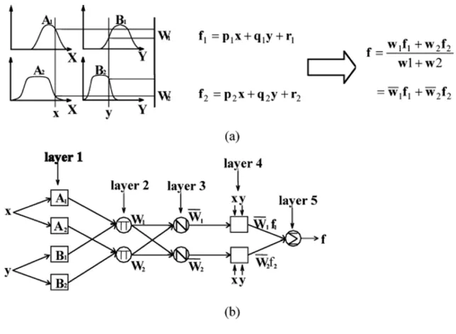
Fig. 1. (a) Type 3 fuzzy reasoning. (b) Equivalent ANFIS (Type 3 ANFIS).
and Baykal, 2001) by different auto-covariance functions. All of these methods have been evaluated only from the mathematical point of view and have often neglected the physical aspects of the geoid. The main advantage of the soft computing techniques is that the physical characteris-tics of the geoid are also taken into consideration to some extent—either explicitly or implicitly.
The study reported here focussed on the geoidal height transformation applications of two soft computing meth-ods, namely the Adaptive Network-based Fuzzy (or in some publications, Adaptive Neuro-Fuzzy) Inference Sys-tem (ANFIS) and Artificial Neural Networks (ANN).
Akyilmazet al.(2003) and Akyilmaz and Kutterer (2004) provide an end-to-end description of the ANFIS approach, and the ANN methodology applied in this study is described by Akyilmazet al.(2004). We have modelled the geoid in Izmir (Turkey) by applying these methodologies. Another mathematical method employed for geoid determination is the fifth-order multi-parameter polynomial approximation (Akyilmazet al., 2003). In addition to employing the soft computing methods and the polynomial approximation, we also applied a least-squares collocation procedure in order to recover the remaining fine structure of the local geoid. In the following sections of this article, we report on the techniques and computing methodology used in our study and compare the soft computing methodologies.
2.
Adaptive Network-based Fuzzy Inference
Sys-tem
The ANFIS has emerged as an extension of fuzzy logic and fuzzy set theory introduced by Zadeh (1965). The bene-fit of ANFIS is that the parameters of the fuzzy sets defined in the inference model are optimised using proper math-ematical algorithms when there is input-output data pairs available on the problem in question. The basic principle of ANFIS can be described as follows: a fuzzy inference
sys-Fig. 2. Meanings of the parameters in the generalised bell membership function.
tem is typically designed by defining linguistic input and output variables as well as an inference rule base. However, the resulting system is just an initial guess for an adequate model. Hence, its premise and consequent parameters have to be tuned based on the given data in order to optimise system performance. In ANFIS, this step is based on a su-pervised learning algorithm (Akyilmazet al., 2003).
An example of an ANFIS with two fuzzy rules are in the following form.
Rule 1: Ifx ∈ A1 andy∈ B1;then f1=p1x+q1y+r1. Rule 2: Ifx ∈ A2 andy∈ B2;then f2=p2x+q2y+r2.
O. AKYILMAZet al.: SOFT COMPUTING OF GEOIDAL HEIGHTS 827
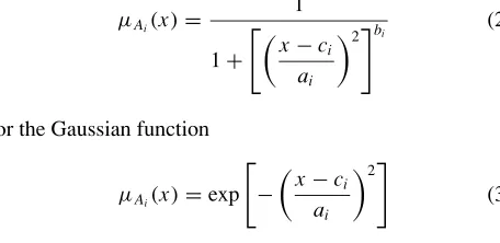
The parameters of the input fuzzy sets (also named as membership functions) Ai, Bj (i = 1, 2 j = 1, 2) are called the premise parameters, whereas the parameters of output functions fi (i =1, 2), i.e. pi,qi andri, are called consequent parameters (Takagi and Sugeno, 1985). The input membership functionμAi(x)is usually chosen to be bell-shaped (Eq. (2)), with the maximum value equal to 1 and the minimum value equal to 0 (such as the generalised bell function; Fig. 2), function) is the parameter set. As the values of these param-eters change, the bell-shaped functions vary accordingly.
The interested reader desiring more information on the set up of ANFIS and the tuning up of the parameters are referred to Jang et al. (1997) and Akyilmaz and Kutterer (2004).
The procedure for the application of ANFIS to geoidal height transformation can be summarized step-by-step as follows:
1) Calculation of the observed geoid heights using Eq. (1). Beforehand, the outliers have to be removed from the data set by statiscal testing of the both GPS and levelling of the derived heights. This is performed during the adjustment of the observations.
2) Separation of the entire data into two independent groups as training and test data sets, respectively. Training data are the reference points which will be used to estimate the ANFIS model parameters, whereas the test data set will be used to validate the es-timated model parameters. The test data set should be distributed as homogenously as possible because the extrapolation is usually problematic. In practice, usu-ally at least 20% of all data points can be selected as the test data.
3) Selection of the input variables. The input variables may be selected as the geographic coordinates of the points or the geographic coordinates and the ellip-soidal heights of the points, as adopted in this study. 4) Assignment of the input membership functions to each
input variable. Different types and numbers of mem-bership functions are possible. However, for geode-tic applications, membership functions of the Gaus-sian type are the most appropriate ones. The optimum number of membership functions for each input vari-able is usually determined by trials regarding the per-formances of the relevant ANFIS models. The output membership functions are the first order polynomials of the input variables. The number of the output mem-bership functions depend on the number of fuzzy rules.
which is the number of all combinations of the input membership functions.
5) Training of the network. After the ANFIS structure (i.e. the number and the type of the input membership functions were determined) has been fixed, the param-eters of both the input membership functions and the output membership functions have to be adjusted iter-atively. There are several mathematical methods that can be used for the training. The hybrid training algo-rithm proposed by Jang (1993) is preferred because of its rapid convergence to the global optimum solution. 6) Validation of the estimated ANFIS parameters. Once
the parameters of the ANFIS are estimated after the training step, they are used to compute the geoid heights at the test data points. The RMS error of the computed geoid heights for the training data and the test data, respectively, should be compatible—in other words, they should be close to each other. If not, the composed set up of the ANFIS is not adequate, and the number of membership functions should be changed (i.e., go to step 3). The trials should be repeated until a compromise between the RMS errors of the training and test data points are achieved.
7) End.
3.
Multilayer Feed-forward Networks
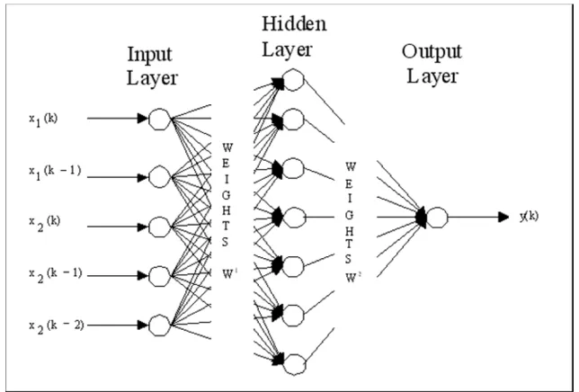
Commonly used artificial neural networks (ANN) are multilayer feed-forward (MLFF) networks. Neural net-works typically consist of many simple neurons located on different layers that operate in cooperation with the neurons on the other layers in order to achieve a good mapping of input-to-output signals. The expression feed-forward em-phasises that the flow of the computation is from input to-wards the output. There are three different types of layers in the concept of neural networks: the input layer (the one to which external stimuli are applied to), the output layer (the layer that results in output) and hidden layers (intermediate computational layers between input and output). Theoreti-cally, there is no limitation given for the number of hidden layers in a network configuration. The absence of such lim-itations, however, has a great effect in the computation time as well as on the number of neurons in hidden layers. There-fore, a compromise has to be found in order to achieve an optimal network configuration with an acceptable conver-gence time and quantitative precision.
Figure 3 provides a sample configuration of a MLFF network with one input, one output and one hidden layer. Note that the network consists of five inputs and one output. When a network configuration is fixed, the parameters of the network, i.e. the weights which link the neurons in con-secutive layers, have to be calculated so that a chosen func-tion of the difference between the actual (desired) output and the output performed by the network is at a minimum. This function is usually called the cost function or perfor-mance index. The most commonly used cost function is the sum of the squares of the residuals:
E= yi(k)−yi(k)
2
(4)
Fig. 3. A schematic representation of a multilayer feed-forward (MLFF) neural network with one hidden layer.
There is a wide spectrum of different mathematical opti-misation tools which are based on the iterative least-squares estimation of the network parameters, such as the steep-est gradient descent, the Levenberg-Marquardt method, the Gauss-Newton method, among others. These are not dis-cussed in detail here but full information can be found in standard textbooks, such as those of Bishop (1995) and Haykin (1994). The procedure for the optimisation of the network parameters is usually calledlearningortrainingin neural computing literature.
Huet al.(2004) applied a two-step approach consisting of the combination of surface function fitting followed by the ANN approximation. In our study we have applied both the conventional ANN approach and the aforementioned hybrid ANN approach introduced by Hu et al. (2004) to the same data to convert the ellipsoidal heights obtained through GPS positioning into the orthometric heights.
The procedure we followed for the application of ANN to geoidal height transformation can be summarized step-by-step as follows:
1) Calculation of the observed geoid heights using Eq. (1). Beforehand, the outliers have to be removed from the data set by statiscal testing of the both GPS and levelling derived heights.
2) Separation of the entire data into two independent groups as training and test data sets, similar to the case in the ANFIS method.
3) Selection of the input variables. The input variables might be selected as the geographic coordinates of the points or as the geographic coordinates and the ellipsoidal heights of the points, as adopted in this study.
4) Setting up the ANN architecture. This step includes the determination of the number of hidden layers and the number of neurons at each hidden layer. The num-ber of input and output layers is known prior to this step as they are equal to the number of input and output
variables, respectively. As a rule, one tries to achieve a reasonable network architecture with as few as possi-ble hidden layers and neurons. This is usually related to the complexity of the process in question. However, for geoidal height transformation, one or two hidden layers are sufficient.
5) Initialization of the training parameters. Before the training has started, some initial parameters have to be defined. These are the initial values of the weights between the neurons in successive layers (see Fig. 3), the “learning rate” and the expected performance of the ANN (also called the “goal” of the ANN) in terms of average RMS error.
The initial values for the weights are usually as-signed by a random number generator. Most of the ANN softwares use random number generators to de-termine the initial weights. However, one can assign the value of 1 to all the weights as the initial values.
The learning rate is in fact the parameter related to the step-size of the iterative adjustment of the weights between the neurons. It is usually selected to be a constant value between 0.01 and 0.10. A high value of the learning rate may yield overtraining, whereas a low value may yield a slow convergence. Therefore, a compromise has to be found for the learning rate. For the numerical example in this study, the value of 0.08 is used.
The goal of the ANN can be defined most simply as the average RMS error of the ellipsoidal heights, which are readily available from the GPS network adjustment. The contribution of the spirit levelling heights to the RMS error of the geoidal undulations can be neglected as they are much more accurate that to the accuracy of the ellipsoidal heights.
itera-O. AKYILMAZet al.: SOFT COMPUTING OF GEOIDAL HEIGHTS 829
tively. There are numerious methods for updating this parameter in ANN applications. The most commonly used one is the so-called “error back-propagation” al-gorithm, which is also known as the “steepest gradi-ent descgradi-ent” algorithm in numerical analysis. In the case of ANNs with a single output (e.g. this study), the Levenberg-Marquardt algorithm can be adopted as it converges more rapidly than the error back-propagation algorithm. Note that all of these training algorithms are gradient-based methods with slight dif-ferences from each other. The training is terminated when the predefined goal (i.e. the average RMS error) is achieved.
7) Validation of the ANN parameters. After the training is terminated, the final estimate of the ANN parame-ters, i.e. the weights, are obtained. These weights are then applied to the test data. The RMS for the test data and that for the training data have to be compatible with each other. If not, the ANN architecture, i.e. the number of the neurons in the hidden layer, has to be al-tered (go to step 4), and the process should be repeated until a compromise between the training and test RMS errors are achieved.
8) End.
4.
Numerical Applications
The data used in this study were collected within the Izmir Geodetic Reference System—2001 project (Ayanet al., 2001). Using these data, we have applied the ANFIS, ANN and fifth-order polynomial approximation methods for geoid determination.
As shown in Fig. 4, the region of Izmir covers an area of approximatelydϕ = 0.30◦ anddλ = 0.56◦. The geoid heights in the area of interest vary from 37.6 to 38.7 m. Although the point density is high in the region, the aver-age accuracy, i.e. the averaver-age RMS error, of the ellipsoidal heights after the adjustment of the network was found to be±3.5 cm. The accuracy of the ellipsoidal heights varies from ±2.8 cm to ±5.0 cm. The region fortunately does not contain very high mountains, and the levelling mea-surements could therefore also be carried out to the points on relatively high hills. Since the soft computing meth-ods cannot handle blunders, adjusted GPS baseline vec-tors were statistically tested and blundered observations re-moved from the data set by an iterative procedure (Baarda, 1968). Hence, the data set do not include any outliers. Ad-ditionally, in terms of Fig. 4, the point distribution is not very optimal. The number of the points with known geoid heights is 310. Of these, 75 uniformly distributed points (approximately 25% of the data set), marked with squares in Fig. 4, were randomly selected to form a test set. The remaining 235 points, marked with filled circles in Fig. 4, were used for training ANFIS and ANN networks.
The first step in our study was to apply ANFIS to trans-form the geoidal height. For these computations, we used the geographic coordinates ϕ,λ, andh as input variables and the geoid height (ξ) as the output of the system. The computations were repeated by using different number of input membership functions of Gaussian type. The differ-ent ANFIS configurations that resulted from these
compu-Fig. 4. Local geoid model in Izmir region.
Fig. 5. Geoid heights obtained from the ANFIS-only method.
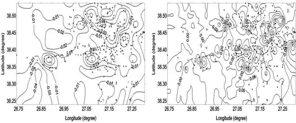
tations were then validated using the test data. After fewer than ten trials, the optimal ANFIS configuration was de-termined to be five, three and one fuzzy sets for the repre-sentation of the input variables, respectively. Figures 5 and 6 show the estimated geoid heights and the distribution of the corresponding errors in the study area, respectively, that were obtained by applying the ANFIS method.
Fig. 6. Differences (residuals) between observed geoid heights and geoid heights computed from the ANFIS-only method.
Fig. 7. Geoid heights obtained from the ANN-only method.
In the above-mentioned applications, the input compo-nents were taken as the ellipsoidal geographic coordinates
ϕ,λ,h; and the output was the geoid height (ξ) (Akyilmaz et al., 2003). In comparison with the ANFIS approxima-tion, it takes a relatively long time to carry out the pro-cedure in the ANN analogy. On the other hand, since the initial weights are randomly drawn values, one can achieve different results for the same ANN configuration after im-plementing different training procedures. Figures 7 and 8 illustrate the estimated geoid heights and the correspond-ing errors in the study area, respectively obtained from the ANN method.
The same data have also been used for the fifth-order polynomial approximation. Table 1 summarises the perfor-mances of the ANFIS and ANN methodologies as well as that of the order polynomial model. Note that the fifth-order polynomial approximation using least squares adjust-ment has been performed twice; first, using all 310 points to determine the coefficients of the polynomial, and
sec-Fig. 8. Differences (residuals) between observed geoid heights and geoid heights computed from the ANN-only method.
ond, using 235 points only to determine the coefficients. The coefficients of the polynomial approximation were also tested for significance; and non-significant ones were then removed from the functional model, and the adjustment was repeated until all the coefficients were statistically signif-icant. Polynomial approximations for higher degrees were also computed; however, there were no reasonable improve-ments in the solutions and to maintain the degree of free-dom, the fifth order polynomial was adopted for this study.
The computations were carried out in twofold. In the first phase, only the proposed methods were directly ap-plied; in the second phase, the computed geoidal undula-tions were assumed to be the deterministic part (trend sur-face) of a least squares collocation (LSC) problem. The unmodelled fine structure of the local geoid surface is then further estimated by the LSC. Several auto-covariance func-tions were applied for this computation, with Hirvonen’s auto-covariance function with a correlation distance of 1 km found to be the most appropriate one of all those tested (Ayan, 1976; Moritz, 1978; Jasecki, 1983).
de-O. AKYILMAZet al.: SOFT COMPUTING OF GEOIDAL HEIGHTS 831 Table 1. Comparison between ANFIS, ANN and the fifth-order approximations (with and without LSC applied).
Approximation type Minimum [m] Maximum [m] Mean [m] Mean absolute Standard Correlation deviation [m] deviation [m] coefficient
235 points ANFIS −0.111 0.098 0.000 0.021 0.030 0.98335
235 points ANN −0.093 0.106 0.001 0.022 0.030 0.98403
235 points fifth order −0.135 0.126 0.000 0.033 0.043 0.97362
310 points fifth order −0.156 0.122 0.000 0.033 0.044 0.96527
75 points ANFIS −0.090 0.141 0.000 0.027 0.037 0.97222
75 points ANFIS+LSC −0.090 0.143 0.000 0.027 0.038 0.97366
75 points ANN −0.158 0.132 0.002 0.029 0.040 0.97981
75 points ANN+LSC −0.152 0.136 0.001 0.028 0.041 0.97311
75 points fifth order −0.122 0.105 0.000 0.035 0.045 0.96462
75 points fifth order+LSC −0.131 0.084 0.000 0.028 0.039 0.96990
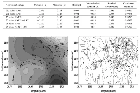
Table 2. Comparison between the hybrid ANFIS and ANN results (with and without LSC applied).
Approximation type Minimum [m] Maximum [m] Mean [m] Mean absolute Standard Correlation deviation [m] deviation [m] coefficient
235 points ANFIS −0.095 0.113 0.000 0.027 0.036 0.97657
235 points ANN −0.106 0.128 0.002 0.025 0.034 0.97841
75 points ANFIS −0.110 0.143 0.002 0.030 0.040 0.96743
75 points ANFIS+LSC −0.106 0.140 0.002 0.028 0.039 0.97427
75 points ANN −0.107 0.126 0.002 0.033 0.043 0.96561
75 points ANN+LSC −0.105 0.134 0.000 0.031 0.042 0.96772
Fig. 9. Geoid heights obtained from the hybrid ANFIS method.
tails of the geoid can be extracted by applying a LSC. This is one of the important findings of the present study.
In the second phase of the computations, the ANFIS and ANN approximations, modified with respect to the method-ology proposed by Huet al.(2004), were applied. First, the 235 points were used as the training group and the fifth-order polynomial coefficients were estimated by the least-squares estimation. Then, using these coefficients, we com-puted approximate geoid height values (ξ0). Deviations from observed (the values computed by taking the differ-ence between the adjusted ellipsoidal heights and levelling heights) geoid height values (ξ) were then calculated and used as the output whereϕ,λand theξ0 were used as the
Fig. 10. Differences (residuals) between observed geoid heights and geoid heights computed from the hybrid ANFIS method.
Fig. 11. Geoid heights obtained from the hybrid ANN method.
Fig. 12. Differences (residuals) between observed geoid heights and geoid heights computed from the hybrid ANN method.
present the results obtained from the hybrid ANN approach. A comparison of the results given in Table 1 shows that the hybrid method yields the worse results, which are due to the computed input observationξ0contributing to the error budget of the ANN and ANFIS models. The best accuracies obtained for the ANFIS and ANN training sets were found to be 0.036 m and 0.034 m, respectively, in terms of stan-dard deviations. Changing the accuracy of the training sets to values equal or lower than 0.030 m yields worse accura-cies for the test set.
From the results given in Table 2, it can be concluded that the quality measures obtained for the training points by the ANFIS methodology is slightly better than those obtained by the ANN approach. As seen, both the minimum and the maximum error values obtained by ANFIS are lower than those produced with the ANN analogy. When the quality measures for the test points are considered, the minimum and maximum values obtained by ANN are better. How-ever, the standard deviation and correlation coefficient
ob-tained by ANFIS are slightly better. We conclude that both methodologies yield identical results. Looking at the re-sults after LSC, again there is no significant improvement both for ANN and ANFIS methods. This is due to the ex-planation mentioned above for the results given in Table 1.
5.
Conclusions
This study deals with the application of Adaptive Net-work based Fuzzy Inference System (ANFIS) and Artificial Neural Networks (ANN) methods to geoidal height trans-formation. We also applied a conventional fifth-order poly-nomial approximation model to determine geoidal height transformation. The outputs obtained by these different ap-proximation methodologies were then compared. A least-squares collocation (LSC) procedure was also applied to the residuals obtained from the all methods.
When the results in Table 1 and Table 2 are compared, it is obvious that it is futile to conduct a pre-process by util-ising a deterministic function which yields reduced values for the observed geoid heights established as the output for the patterns in both ANFIS and ANN methodologies. The results given by Huet al.(2004) are quite precise, possibly because the study field covered a small and considerably smooth area and the height differences between the geode-tic points were at a low level.
We found that ANFIS approximation yields better results than the classical ANN approximation and the conventional fifth-order polynomial model. However, the modified ANN analogy introduced by Huet al.(2004) produces identical results with the ANFIS approximation.
A number of aspects of ANFIS have to be strictly con-trolled when using this application. One of these is that the number of parameters, including both premise and conse-quent, has to be less than the number of training data pairs. This avoids the overfitting phenomenon, which does not al-low generalisation of the established fuzzy inference sys-tem.
Regardless of which method is used, the efficiency of the approximation is limited at least by the accuracy of the el-lipsoidal heights obtained from the adjustment of the net-work as it has the dominant effect on the geoidal undula-tions or the height anomaly. This means that it is not pos-sible to achieve an approximation of the accuracy that is better than the accuracy of the ellipsoidal heights. Given this limitation, the RMS error obtained by ANFIS is very close to the accuracy of adjusted ellipsoidal heights. Point distribution is also an important factor for the approxima-tion quality. It should also be stated that the convergence of ANFIS is considerably faster than that of ANN. Moreover, the ANFIS approximation requires fewer parameters than ANN. For example, ANFIS modelling without polynomial fitting (Table 1) contains 78 parameters to be updated by the training runs. In the case of ANFIS combined with the pre-process (in Table 2), this is 44. However, in the case of ANN, the number of parameters is 507 for both ANN approaches given in Tables 1 and 2.
O. AKYILMAZet al.: SOFT COMPUTING OF GEOIDAL HEIGHTS 833
computing methods, such as ANN and ANFIS, tend to de-scribe the surface in piecewise (either linear or non-linear) functions, and the entire study area is covered by these lo-cally best fitting piecewise functions.
A study of Figs. 5–12 reveals that the ANFIS-only method provides a smoother view of the geoid heights as well as the corresponding errors in the study area. This re-sult is due to the characteristics of the ANFIS method. In contrast, the hybrid-ANFIS results (Figs. 9 and 10), i.e. the application of LSC to the ANFIS residuals, has a corrupting effect on the smoothness and the distribution of the geoid height errors.
Acknowledgments. Dr. Takeshi Sagiya and the two anonymous referees are gratefully acknowledged for their constructive com-ments which greatly improved the quality of the manuscript.
References
Akyilmaz, O. and H. Kutterer, Prediction of Earth rotation parameters by fuzzy inference system,J. Geod.,78, 82–93, doi:10.1007/s00190-004-0374-5, 2004.
Akyilmaz, O., T. Ayan, and M. T. ¨Ozl¨udemir, Geoid surface approximation by using Adaptive Network based Fuzzy Inference Systems,AVN,8–9, 308–315, 2003.
Akyilmaz, O., R. N. C¸ elik, N. Apaydin, and T. Ayan, GPS monitoring of the Fatih Sultan Mehmet suspension bridge by using assessment meth-ods of neural networks. The International Archives of the Photogram-metry, Remote Sensing,Spatial Inf. Sci.,34, 702–707, 2004.
Ayan, T., Astrogeodetic Geoid Determination for the Area of Turkey, Ph.D. dissertation, Karlsruhe, Germany, 1976 (in German).
Ayan, T., R. Deniz, R. N. C¸ elik, H. H. Denli, M. T. ¨Ozl¨udemir, S. Erol, B. ¨
Oz¨oner, O. Akyilmaz, and C. G¨uney, Izmir geodetic reference system— 2001 (IzJRS-2001),Technical Report, Istanbul Technical University, Turkey, 2001 (in Turkish).
Baarda, W., A testing procedure for use in geodetic networks,Netherlands
Geodetic Commission, Publications in Geodesy, New Series,2(5), Delft, The Netherlands, 1968.
Bishop, C. M.,Neural networks for pattern recognition, Oxford University Press, 1995.
Engelis, T., R. H. Rapp, and Y. Bock, Measuring orthometric height dif-ferences with GPS and gravity data,Manuscripta Geodaetica,10(3), 187–194, 1985.
Featherstone, W. E., Absolute and relative testing of gravimetric geoid models using Global Positioning System and orthometric height data,
Comput. Geosci.,27, 807–814, doi:10.1016/S0098-3004(00)00169-2, 2001.
Haykin, S., Neural networks: a comprehensive foundation, Maxwell Macmillan Int., New York, 1994.
Hu, W., Y. Sha, and S. Kuang, New method for transforming Global Positioning System height into normal height based on Neural Network,
J. Surv. Eng.,130(1), 36–39, 2004.
Jang, J. S., ANFIS: Adaptive-Network-Based Fuzzy Inference System,
IEEE Trans. Systems Man Cybernetics,23, 665–685, 1993.
Jang, J. S., C. Sun, and E. Mizutani,Neuro-Fuzzy and Soft Computing, Prentice-Hall, Englewood Cliffs, NJ, 1997.
Jasecki, M., The covariance function in the process of developing geodetic data, Geodesy Cartography,PWN,32(4), 283–292, Warsaw, 1983. Kuhar, M., B. Stopar, G. Turk, and T. Ambroˇziˇc, The use of artificial neural
network in geoid surface approximation,AVN,1, 22–27, 2001. Moritz, H., Least-squares collocation,Rev. Geoph. Space Physics,16(3),
1978.
Seeber, G.,Satellite Geodesy, 2nd revision edition, Walter de Gruyter Inc., 2003.
Takagi, T. and M. Sugeno, Fuzzy identification of systems and its applica-tion to modelling and control,IEEE Trans. Systems Man Cybernetics, 15, 116–132, 1985.
Yanalak, M. and O. Baykal, Transformation of ellipsoidal heights to local levelling heights,ASCE J. Surv. Eng.,127(3), 90–103, 2001.
Zadeh, L. A., Fuzzy sets,Inf. Control,8, 338–353, 1965