Theory of nth order linear general quantum difference equations

(1)

R E S E A R C H

Open Access

Theory of

n

th-order linear general

quantum difference equations

Nashat Faried

1

_{, Enas M. Shehata}

2*

_{and Rasha M. El Zafarani}

1

*_{Correspondence:}

[email protected] 2_{Department of Mathematics,}

Faculty of Science, Menouﬁa University, Shibin El-Koom, Egypt Full list of author information is available at the end of the article

Abstract

In this paper, we derive the solutions of homogeneous and non-homogeneous nth-order linear general quantum difference equations based on the general quantum difference operatorDβ which is defined byDβf(t) = (f(β(t)) –f(t))/(β(t) –t),

β

(t)=t, where

β

is a strictly increasing continuous function defined on an interval I⊆Rthat has only one fixed points0∈I. We also give the sufficient conditions for the

existence and uniqueness of solutions of the

β

-Cauchy problem of these equations. Furthermore, we present the fundamental set of solutions when the coeﬃcients are constants, the

β-Wronskian associated with

Dβ, and Liouville’s formula for the

β

-diﬀerence equations. Finally, we introduce the undetermined coeﬃcients, the variation of parameters, and the annihilator methods for the non-homogeneous

β

-diﬀerence equations.

MSC: Primary 39A10; 39A13; 39A70; secondary 47B39

Keywords: A general quantum diﬀerence operator;nth-order linear general quantum diﬀerence equations;

β

-Wronskian; Homogeneous quantum diﬀerence equations; Non-homogeneous quantum diﬀerence equations

1 Introduction

Quantum difference operator allows us to deal with sets of non-differentiable functions. Its applications are used in many mathematical fields such as the calculus of variations, orthogonal polynomials, basic hypergeometric functions, quantum mechanics, and the theory of scale relativity; see, e.g., [3,5,7,13,14].

The general quantum diﬀerence operatorDβgeneralizes the Jacksonq-diﬀerence

oper-atorDqand the Hahn diﬀerence operatorDq,ω, see [1,2,4,8,12]. It is deﬁned, in [10, p.

6], by

Dβf(t) = ⎧ ⎨ ⎩

f(β(t))–f(t)

β(t)–t , t=s0,

f(s0), t=s0,

wheref :I→Xis a function deﬁned on an interval I⊆R, Xis a Banach space, and

β:I→Iis a strictly increasing continuous function defined onIthat has only one fixed points0∈I and satisfies the inequality (t–s0)(β(t) –t)≤0 for allt∈I. The function

f is said to beβ-diﬀerentiable onI if the ordinary derivativefexists ats0. The general

quantum diﬀerence calculus was introduced in [10]. The exponential, trigonometric, and

(2)

hyperbolic functions associated withDβwere presented in [9]. The existence and

unique-ness of solutions of the ﬁrst-orderβ-initial value problem were established in [11]. In [6], the existence and uniqueness of solutions of theβ-Cauchy problem of the second-order

β-difference equations were proved. Also, a fundamental set of solutions for the second-order linear homogeneousβ-difference equations when the coefficients are constants was constructed, and the different cases of the roots of their characteristic equations were stud-ied. Moreover, the Euler–Cauchyβ-difference equation was derived.

The organization of this paper is briefly summarized in the following. In Sect.2, we present the needed preliminaries of the β-calculus from [6,9–11]. In Sect. 3, we give the sufficient conditions for the existence and uniqueness of solutions of theβ-Cauchy problem of thenth-orderβ-difference equations. Also, we construct the fundamental set of solutions for the homogeneous linearβ-difference equations when the coefficientsaj

(0≤j≤n) are constants. Furthermore, we introduce theβ-Wronskian which is an effec-tive tool to determine whether the set of solutions is a fundamental set or not and prove its properties. Finally, we study the undetermined coefficients, the variation of parameters, and the annihilator methods for the non-homogeneous linearβ-difference equations.

Throughout this paper,Jis a neighborhood of the unique ﬁxed points0ofβ,S(y0,b) =

{y∈X:y–y0 ≤b}, andR={(t,y)∈I×X:|t–s0| ≤a,y–y0 ≤b}is a rectangle, where

a,bare ﬁxed positive real numbers,Xis a Banach space. Furthermore,Dn

βf =Dβ(Dnβ–1f),

n∈N0=N∪{0}, wheref isβ-diﬀerentiablentimes overI,Nis the set of natural numbers.

We use the symbolTfor the transpose of the vector or the matrix.

2 Preliminaries

Lemma 2.1([10]) The following statements are true:

(i) The sequence of functions{βk₍_t₎_}∞

k=0converges uniformly to the constant function

ˆ

β(t) :=s0on every compact intervalV⊆Icontainings0.

(ii) The series∞_k₌₀|βk(t) –βk+1(t)|is uniformly convergent to|t–s0|on every compact

intervalV⊆Icontainings0.

Lemma 2.2([10]) If f :I→Xis a continuous function at s0,then the sequence{f(βk(t))}∞k=0

converges uniformly to f(s0)on every compact interval V⊆I containing s0.

Theorem 2.3([10]) If f :I→Xis continuous at s0,then the series

∞

k=0(βk(t)–βk+1(t))×

f(βk₍_t₎₎_{is uniformly convergent on every compact interval V}_⊆_{I containing s} 0.

Theorem 2.4([10]) Assume that f :I→Xand g:I→Rareβ-diﬀerentiable at t∈I.

Then:

(i) The productfg:I→Xisβ-diﬀerentiable attand

Dβ(fg)(t) =

Dβf(t)

g(t) +fβ(t)Dβg(t)

=Dβf(t)

gβ(t)+f(t)Dβg(t), (ii) f/gisβ-diﬀerentiable attand

Dβ(f/g)(t) =

(Dβf(t))g(t) –f(t)Dβg(t)

g(t)g(β(t)) ,

(3)

Theorem 2.5([10]) Assume that f :I→Xis continuous at s0.Then the function F deﬁned

by

F(t) = ∞

k=0

βk(t) –βk+1(t)fβk(t), t∈I (2.1)

is aβ-antiderivative of f with F(s0) = 0.Conversely,aβ-antiderivative F of f vanishing at

s0is given by(2.1).

Deﬁnition 2.6([10]) Theβ-integral off :I→Xfromatob,a,b∈I, is deﬁned by

b

a

f(t)dβt=

b

s0

f(t)dβt–

a

s0

f(t)dβt,

where

x

s0

f(t)dβt=

∞

k=0

βk(x) –βk+1(x)fβk(x), x∈I,

provided that the series converges atx=aandx=b.f is calledβ-integrable onIif the series converges ataandbfor alla,b∈I. Clearly, iff is continuous ats0∈I, thenf is

β-integrable onI.

Deﬁnition 2.7([9]) Theβ-exponential functionsep,β(t) andEp,β(t) are deﬁned by

ep,β(t) =

1

_∞

k=0[1 –p(βk(t))(βk(t) –βk+1(t))]

(2.2)

and

Ep,β(t) =

∞

k=0

1 +pβk(t)βk(t) –βk+1(t), (2.3)

wherep:I→Cis a continuous function ats0,ep,β(t) = _E 1

–p,β(t).

The both products in (2.2) and (2.3) are convergent to a non-zero number for everyt∈I

since∞_k₌₀|p(βk(t))(βk(t) –βk+1(t))|is uniformly convergent.

Deﬁnition 2.8([9]) Theβ-trigonometric functions are deﬁned by

cosp,β(t) =

eip,β(t) +e–ip,β(t)

2 ,

sin_p_,β(t) =

eip,β(t) –e–ip,β(t)

2i ,

Cos_p_,β(t) =

Eip,β(t) +E–ip,β(t)

2 ,

and Sinp,β(t) =

Eip,β(t) –E–ip,β(t)

(4)

Theorem 2.9([9]) Theβ-exponential functions ep,β(t)and Ep,β(t)are the unique solutions

of the ﬁrst-orderβ-diﬀerence equations

Dβy(t) =p(t)y(t), y(s0) = 1,

Dβy(t) =p(t)y

β(t), y(s0) = 1,

respectively.

Theorem 2.10([9]) Assume that f :I→Xis continuous at s0.Then the solution of the

following equation Dβy(t) =p(t)y(t) +f(t),y(s0) =y0∈X,has the form

y(t) =ep,β(t)

y0+ t

s0

f(τ)E–p,β

β(τ)dβτ

.

Theorem 2.11([11]) Let z∈Cbe a constant.Then the functionφ(t)deﬁned by

φ(t) = ∞

k=0

zkαk(t)

is the unique solution of theβ-IVP

Dβy(t) =zy(t), y(s0) = 1,

where

αk(t) = ⎧ ⎪ ⎪ ⎪ ⎨ ⎪ ⎪ ⎪ ⎩

∞

i1,i2,i3,...,ik–1=0(

k–1

l=1(β,β)l_j₌₁ij)(β k–1

j=1ij

(t) –s0), if k≥2,

t–s0, if k= 1,

1, if k= 0,

with(β,β)i=βi(t) –βi+1(t).

Proposition 2.12([11]) Let z∈C.Theβ-exponential function ez,β(t)has the expansion

ez,β(t) =

∞

k=0

zk_α k(t).

Theorem 2.13([11]) Assume that f :R→Xis continuous at(s0,y0)∈R and satisﬁes the

Lipschitz condition(with respect to y)

f(t,y1) –f(t,y2)≤Ly1–y2 for all(t,y1), (t,y2)∈R,

where L is a positive constant.Then the sequence deﬁned by

φk+1(t) =y0+ t

s0

fτ,φk(τ)

(5)

converges uniformly on the interval|t–s0| ≤δto a functionφ,the unique solution of the

β-IVP

Dβy(t) =f(t,y), y(s0) =y0, t∈I, (2.5)

whereδ=min{a,_Lbb₊_M,ρ_L}withρ∈(0, 1)and M=sup₍_t_,_y₎_∈_Rf(t,y)<∞,ρ∈(0, 1).

Theorem 2.14([6]) Let fi(t,y1,y2) :I×

2

i=1Si(xi,bi)→X,s0∈I such that the following

conditions are satisﬁed:

(i) Foryi∈Si(xi,bi),i= 1, 2,fi(t,y1,y2)are continuous att=s0.

(ii) There is a positive constantAsuch that,fort∈I,yi,y˜i∈Si(xi,bi),i= 1, 2,the following Lipschitz condition is satisﬁed:

fi(t,y1,y2) –fi(t,y˜1,˜y2)≤A 2

i=1

yi–˜yi.

Then there exists a unique solution of theβ-initial value problemβ-IVP Dβyi(t) =fi

t,y1(t),y2(t)

, yi(s0) =xi∈X, i= 1, 2,t∈I. Corollary 2.15([6]) Let f(t,y1,y2)be a function deﬁned on I×

2

i=1Si(xi,bi)such that the

following conditions are satisﬁed:

(i) For any values ofyi∈Si(xi,bi),i= 1, 2,f is continuous att=s0.

(ii) f satisﬁes the Lipschitz condition f(t,y1,y2) –f(t,y˜1,˜y2)≤A

2

i=1

yi–y˜i,

where A> 0,yi,˜yi∈Si(xi,bi),i= 1, 2,and t∈I.Then

D2βy(t) =f

t,y(t),Dβy(t)

, Diβ–1y(s0) =xi, i= 1, 2,

has a unique solution on[s0,s0+δ].

Corollary 2.16([6]) Assume that the functions aj(t) :I→C,j= 0, 1, 2,and b(t) :I→X

satisfy the following conditions:

(i) aj(t),j= 0, 1, 2,andb(t)are continuous ats0witha0(t)= 0for allt∈I,

(ii) aj(t)/a0(t)is bounded onI,j= 1, 2.Then

a0(t)D2βy(t) +a1(t)Dβy(t) +a2(t)y(t) =b(t), Diβ–1y(s0) =xi, xi∈X,i= 1, 2,

has a unique solution on a subinterval J⊆I,s0∈J. 3 Main results

In this section, we give the sufficient conditions for the existence and uniqueness of solu-tions of theβ-Cauchy problem of thenth-orderβ-difference equations. We also present the fundamental set of solutions for the homogeneous linearβ-difference equations when the coefficientsaj(0≤j≤n) are constants. Furthermore, we introduce theβ-Wronskian.

(6)

3.1 Existence and uniqueness of solutions

Theorem 3.1 Let I be an interval containing s0,fi(t,y1, . . . ,yn) :I× n

i=1Si(xi,bi)→X,

such that the following conditions are satisﬁed:

(i) Foryi∈Si(xi,bi),i= 1, . . . ,n,fi(t,y1, . . . ,yn)are continuous att=s0.

(ii) There is a positive constantAsuch that,fort∈I,yi,y˜i∈Si(xi,bi),i= 1, . . . ,n,the following Lipschitz condition is satisﬁed:

fi(t,y1, . . . ,yn) –fi(t,y˜1, . . . ,y˜n)≤A n

i=1

yi–y˜i.

Then there exists a unique solution of theβ-initial value problemβ-IVP

Dβyi(t) =fi

t,y1(t), . . . ,yn(t)

, yi(s0) =xi∈X, i= 1, . . . ,n,t∈I.

Proof See the proof of Theorem2.14. The proof of the following two corollaries is the same as the proof of Corollaries2.15,

2.16.

Corollary 3.2 Let f(t,y1, . . . ,yn)be a function deﬁned on I×ni=1Si(xi,bi)such that the

following conditions are satisﬁed:

(i) For any values ofyr∈Sr(xr,br),f is continuous att=s0.

(ii) f satisﬁes the Lipschitz condition

f(t,y1, . . . ,yn) –f(t,y˜1, . . . ,y˜n)≤A n

i=1

yi–y˜i,

where A> 0,yi,˜yi∈Si(xi,bi),i= 1, . . . ,n,and t∈I.Then

Dnβy(t) =f

t,y(t),Dβy(t), . . . ,Dnβ–1y(t)

,

Diβ–1y(s0) =xi, i= 1, . . . ,n,

(3.1)

has a unique solution on[s0,s0+δ].

The following corollary gives us the suﬃcient conditions for the existence and unique-ness of solutions of theβ-Cauchy problem (3.1).

Corollary 3.3 Assume that the functions aj(t) :I→C,j= 0, 1, . . . ,n,and b(t) :I→X

sat-isfy the following conditions:

(i) aj(t),j= 0, 1, . . . ,n,andb(t)are continuous ats0witha0(t)= 0for allt∈I,

(ii) aj(t)/a0(t)is bounded onI,j= 1, . . . ,n.Then

a0(t)Dnβy(t) +a1(t)Dβn–1y(t) +· · ·+an(t)y(t) =b(t),

Di_β–1y(s0) =xi, i= 1, . . . ,n,

(7)

3.2 Homogeneous linear

β

-difference equations

Consider thenth-order homogeneous linearβ-diﬀerence equation

a0(t)Dnβy(t) +a1(t)Dnβ–1y(t) +· · ·+an–1(t)Dβy(t) +an(t)y(t) = 0, (3.2)

where the coeﬃcients aj(t), 0≤j≤n, are assumed to satisfy the conditions of

Corol-lary3.3. Equation (3.2) may be written asLny= 0, where

Ln=a0(t)Dβn+a1(t)Dβn–1+· · ·+an–1(t)Dβ+an(t).

The following lemma is an immediate consequence of Corollary3.3.

Lemma 3.4 If y is a solution of equation(3.2)such that Diβ–1y(s0) = 0, 1≤i≤n,then y(t) =

0for all t∈J.

Theorem 3.5 The nth-order homogeneous linear scalar β-diﬀerence equation (3.2) is equivalent to the ﬁrst-order homogeneous linear system of the form

DβY(t) =A(t)Y(t),

where

Y=

⎛ ⎜ ⎜ ⎝

y1

.. .

yn ⎞ ⎟ ⎟

⎠ and A=

⎛ ⎜ ⎜ ⎜ ⎜ ⎝

0 1 . . . 0

..

. ... . . . ...

0 0 1

–an

a0 – an–1

a0 . . . – a1 a0

⎞ ⎟ ⎟ ⎟ ⎟ ⎠.

Proof Let

y1=y,

y2=Dβy,

.. .

yn–1=Dnβ–2y,

yn=Dnβ–1y.

(3.3)

β-diﬀerentiating (3.3), we have

Dβy=Dβy1, Dβ2y=Dβy2, . . . , Dβn–1y=Dβyn–1, Dnβy=Dβyn. (3.4)

Then

Dβy1=y2, Dβy2=y3, . . . , Dβyn–1=yn. (3.5)

Sincea0(t)= 0 onJ, (3.2) is equivalent to

Dnβy= –

an(t)

a0(t)

y–an–1(t)

a0(t)

Dβy–· · ·–

a1(t)

a0(t)

(8)

from (3.3) and (3.4), we have

This is equivalent to the homogeneous linear vectorβ-diﬀerence equation

DβY(t) =A(t)Y(t), (3.8)

Theorem 3.6 Consider equation(3.2)and the corresponding system(3.8).If f is a solution of (3.2)on J,thenφ= (f,Dβf, . . . ,Dβn–1f)T is a solution of (3.8)on J.Conversely, ifφ=

(φ1, . . . ,φn)Tis a solution of (3.8)on J,then its ﬁrst componentφ1is a solution f of (3.2)on

J andφ= (f,Dβf, . . . ,Dnβ–1f)T.

Proof Suppose thatf satisﬁes equation (3.2). Then

(9)

Comparing (3.11) with (3.7),φdefined by (3.10) satisfies system (3.7). Conversely, suppose thatφ(t) = (φ1(t), . . . ,φn(t))Tsatisfies system (3.7) onJ. Then (3.11) holds for allt∈J. The

ﬁrstn– 1 equations of (3.11) give

φ2(t) =Dβφ1(t),

φ3(t) =Dβφ2(t) =D2βφ1(t),

.. .

φn(t) =Dβφn–1(t) =D2βφn–2(t) =· · ·=Dnβ–1φ1(t),

(3.12)

and soDβφn(t) =Dnβφ1(t). The last equation of (3.11) becomes

a0(t)Dnβφ1(t) +a1(t)Dnβ–1φ1(t) +· · ·+an–1(t)Dβφ1(t) +an(t)φ1(t) = 0.

Thus φ1 is a solution f of equation (3.2); and moreover, (3.12) shows that φ(t) =

(f(t),Dβf(t), . . . ,Dnβ–1f(t))T.

The following corollary is an immediate consequence of Theorem3.6.

Corollary 3.7 If f is the solution of equation(3.2)on J satisfying the initial condition Diβ–1f(s0) =xi, 1≤i≤n,thenφ= (f,Dβf, . . . ,Dβn–1f)T is the solution of system(3.8)on J

satisfying the initial conditionφ(s0) = (x1, . . . ,xn)T.Conversely,ifφ= (φ1, . . . ,φn)Tis the

so-lution of(3.8)on J satisfying the initial conditionφ(s0) = (x1, . . . ,xn)T,thenφ1is the solution

f of (3.2)on J satisfying the initial condition Di–1

β f(s0) =xi, 1≤i≤n.

Theorem 3.8 A linear combination y=m_k₌₁ckykof m solutions y1, . . . ,ymof the

homoge-neous linearβ-diﬀerence equation(3.2)is also a solution of it,where c1, . . . ,cmare arbitrary

constants.

Proof The proof is straightforward.

Deﬁnition 3.9(A fundamental set) A set ofnlinearly independent solutions of then th-order homogeneous linearβ-diﬀerence equation (3.2) is called a fundamental set of equa-tion (3.2).

By the theory of diﬀerential equations, we can easily prove the following theorems.

Theorem 3.10 If the solutions y1, . . . ,ynof the homogeneous linearβ-diﬀerence equation

(3.2)are linearly independent on J,then the corresponding solutions

φ1=

y1,Dβy1, . . . ,Dnβ–1y1

T

, . . . , φn=

yn,Dβyn, . . . ,Dnβ–1yn T

of system(3.8)are linearly independent on J;and conversely.

Theorem 3.11 Any arbitrary solution y of homogeneous linearβ-diﬀerence equation(3.2)

(10)

Now, we are concerned with constructing the fundamental set of solutions of equation (3.2) when the coeﬃcients are constants. Equation (3.2) can be written as

Lny(t) =a0Dnβy(t) +a1Dnβ–1y(t) +· · ·+any(t) = 0, (3.13)

whereaj, 0≤j≤n, are constants. From Theorem3.5, equation (3.13) is equivalent to the

system

DβY(t) =AY(t), (3.14)

where

A=

⎛ ⎜ ⎜ ⎜ ⎜ ⎝

0 1 . . . 0

..

. ... . . . ...

0 0 1

–an

a0 – an–1

a0 . . . – a1 a0

⎞ ⎟ ⎟ ⎟ ⎟ ⎠.

The characteristic polynomial of equation (3.13) is given by

P(λ) =det(λI–A) =a0λn+a1λn–1+· · ·+an, (3.15)

whereIis the unit square matrix of ordern,λi, 1≤i≤k, are distinct roots ofp(λ) = 0 of

multiplicitymi, so that k

i=1mi=n.

Theorem 3.12 Let A be a constant n×n matrix.Then the function(t)deﬁned by

(t) = ∞

r=0

Arαr(t)

is the unique solution of theβ-IVP

DβY(t) =AY(t), Y(s0) =I,

whereIis the unit square matrix of order n and

αr(t) = ⎧ ⎪ ⎪ ⎪ ⎨ ⎪ ⎪ ⎪ ⎩

_∞

i1,i2,i3,...,ir–1=0(

r–1 l=1(β,β)l

j=1ij)(β r–1

j=1ij₍_t_{) –}_s

0), if r≥2,

t–s0 if r= 1,

I, if r= 0,

with(β;β)i=βi(t) –βi+1(t).

Proof By using the successive approximations, with choosing0(t) =I, we have the

(11)

Corollary 3.13 Let A be a constant n×n matrix with characteristic polynomial(3.15),

Proof The proof is straightforward. We have from the previous that

yi(t) =eλi,β(t) = ∞

r=0

λr_iαr(t), 1≤i≤k,

forms a fundamental set of solutions of equation (3.13).

Example3.14 Consider the homogeneous linear system

DβY(t) =

are the solutions of (3.16). The general solution of system (3.16) is

Y(t) =c1

Example3.15 Consider the homogeneous linear system

(12)

whereλ1=λ2=λ3= 2. Then

The general solution of system (3.17) is

(13)

Lemma 3.17 Let y1(t), . . . ,yn(t)be n-timesβ-diﬀerentiable functions deﬁned on I.Then,

Proof We prove by induction onn. The lemma is trivial whenn= 1. Then suppose that it is true forn=k. Our objective is to show that it holds forn=k+ 1.

and from the induction hypothesis we have

(14)

×

satisfies the first-orderβ-difference equation

DβWβ(t) = –P(t)Wβ(t), ∀t∈J\{s0}, (3.20)

Proof First, we show by induction that the following relation

(15)

(16)

(17)

=

n

k=1

(–1)2(k–1)t–β(t)k–1

–ak(t)

a0(t)

Wβ(t)

= –

n–1

k=0

t–β(t)k

ak+1(t)

a0(t)

Wβ(t) = –P(t)Wβ(t),

which is the desired result.

The following theorem gives us Liouville’s formula forβ-diﬀerence equations.

Theorem 3.19 Assume that(β(t) –t)P(t)= 1,t∈J.Then theβ-Wronskian of any set of solutions{yi(t)}ni=1,valid in J,is given by

Wβ(t) =

Wβ(s0)

∞

k=0[1 +P(βk(t))(βk(t) –βk+1(t))]

, t∈J. (3.25)

Proof Relation (3.20) implies that

Wβ

β(t)=1 +t–β(t)P(t)Wβ(t), t∈J\{s0}.

Hence,

Wβ(t) =

Wβ(β(t))

1 + (t–β(t))P(t)

= Wβ(β

m₍_t₎₎ m–1

k=0[1 +P(βk(t))(βk(t) –βk+1(t))]

, m∈N.

Takingm→ ∞, we get

Wβ(t) =

Wβ(s0)

∞

k=0[1 +P(βk(t))(βk(t) –βk+1(t))]

, t∈J.

Example3.20 We calculate theβ-Wronskian of theβ-diﬀerence equation

D2βy(t) +y(t) = 0. (3.26)

The functionsy1(t) =cos1,β(t) andy2(t) =sin1,β(t) are solutions of equation (3.26) subject

to the initial conditionsy1(s0) = 1,Dβy1(s0) = 0,y2(s0) = 0,Dβy2(s0) = 1, respectively. Here,

P(t) = (t–β(t)). So, (β(t) –t)P(t)= 1 for allt=s0. Since

Wβ(s0) =

cos1,β(s0) sin1,β(s0)

sin1,β(s0) cos1,β(s0)

=

1 0

0 1

= 1.

Therefore,Wβ(t) = ∞ 1

k=0[1+(βk(t)–βk+1(t))2].

The following corollary can be deduced directly from Theorem3.19.

Corollary 3.21 Let{yi}ni=1be a set of solutions of equation(3.2)in J.Then Wβ(t)has two

(18)

(i) Wβ(t)= 0inJif and only if{yi}ni=1is a fundamental set of equation(3.2)valid inJ.

(ii) Wβ(t) = 0inJif and only if{yi}ni=1is not a fundamental set of equation(3.2)valid

inJ.

3.4 Non-homogeneous linear

β

-difference equations

Thenth-order non-homogeneous linearβ-diﬀerence equation has the form

a0(t)Dnβy(t) +a1(t)Dnβ–1y(t) +· · ·+an–1(t)Dβy(t) +an(t)y(t) =b(t), (3.27)

where the coeﬃcientsaj(t), 0≤j≤n, andb(t) are assumed to satisfy the conditions of

Corollary3.3. We may write this as

Lny=b(t), (3.28)

where, as before,Ln=a0(t)Dβn+a1(t)Dβn–1+· · ·+an–1(t)Dβ+an(t).

By the theory of diﬀerential equations, ify1(t) andy2(t) are two solutions of the

non-homogeneous equation (3.28), theny1±y2 is a solution of the corresponding

homoge-neous equation (3.2). Also, by Theorem3.11, ify1(t), . . . ,yn(t) form a fundamental set for

equation (3.2) andϕ(t) is a particular solution of equation (3.27), then for any solution of equation (3.27), there are constantsc1, . . . ,cnsuch that

y(t) =ϕ(t) +c1y1(t) +· · ·+cnyn(t). (3.29)

Therefore, if we can ﬁnd any particular solutionϕ(t) of equation (3.27), then (3.29) gives a general formula for all solutions of equation (3.27).

Theorem 3.22 Letϕibe a particular solution of Lny=bi(t),i= 1, . . . ,m.Then m

i=1ζiϕiis

a particular solution of the equation Lny= m

i=1ζibi(t),whereζ1, . . . ,ζmare constants.

Proof The proof is straightforward.

3.4.1 Method of undetermined coeﬃcients

We will illustrate the method of undetermined coeﬃcients when the coeﬃcientsaj(0≤

j≤n) of the non-homogeneous linearβ-diﬀerence equation (3.27) are constants by simple examples.

Example3.23 Find a particular solution of

D2βy(t) – 3Dβy(t) – 4y(t) = 3e2,β(t). (3.30)

Assume that

ϕ(t) =ζe2,β(t), (3.31)

where the coeﬃcientζ is a constant to be determined. To ﬁndζ, we calculate

(19)

by substituting with equations (3.31), (3.32) in equation (3.30). Thus a particular solution is

ϕ(t) = –1/2e2,β(t).

In the following example, we refer the reader to see the different cases of the roots of the characteristic equation of second-order linear homogeneousβ-difference equation when the coefficients are constants, see [6].

Example3.24 Find the general solution of

D2βy– 3Dβy– 4y= 2sin1,β(t). (3.33)

The corresponding homogeneous equation of (3.33) is

D2βy– 3Dβy– 4y= 0. (3.34)

Then the characteristic polynomial of (3.34) is

P(λ) =λ2– 3λ– 4 = 0. (3.35)

Therefore,

yh(t) =c1e4,β(t) +c2e–1,β(t).

Now, assume that

ϕ(t) =ζ1sin1,β(t) +ζ2cos1,β(t), (3.36)

whereζ1andζ2are to be determined. Then

Dβϕ(t) =ζ1cos1,β(t) –ζ2sin1,β(t),

D2βϕ(t) = –ζ1sin1,β(t) –ζ2cos1,β(t).

(3.37)

By substituting with equations (3.36), (3.37) in equation (3.33), we get a particular solution

ϕ(t) = –5/17sin1,β(t) + 3/17cos1,β(t).

Then the general solution of (3.33) is

y(t) =c1e4,β(t) +c2e–1,β(t) – 5/17sin1,β(t) + 3/17cos1,β(t).

(20)

D2βy– 2Dβy– 3y= 2e1,β(t) – 10sin1,β(t). (3.38)

The corresponding homogeneous equation of (3.38) has the solution

yh(t) =c1e3,β(t) +c2e–1,β(t).

The non-homogeneous term is the linear combination 2e1,β(t) – 10sin1,β(t) of the two

functions given bye1,β(t) andsin1,β(t).

Let

ϕ(t) =c1e1,β(t) +c2sin1,β(t) +c3cos1,β(t) (3.39)

be a particular solution of (3.38). Then

Dβϕ(t) =c1e1,β(t) +c2cos1,β(t) –c3sin1,β(t),

D2βϕ(t) =c1e1,β(t) –c2sin1,β(t) –c3cos1,β(t),

(3.40)

wherec1,c2,c3are undetermined coeﬃcients. By substituting with (3.39), (3.40) in (3.38),

we have the particular solutionϕ(t) = –1/2e1,β(t) + 2sin1,β(t) –cos1,β(t). Thus the general

solution of (3.38) is

y(t) =c1e3,β(t) +c2e–1,β(t) – 1/2e1,β(t) + 2sin1,β(t) –cos1,β(t).

D2βy– 3Dβy+ 2y=e3,β(t)sin4,β(t). (3.41)

The corresponding homogeneous equation of (3.41) has the solution

yh(t) =c1e2,β(t) +c2e1,β(t).

Let

ϕ(t) =Ae3,β(t)sin4,β(t) +Be3,β(t)cos4,β(t) (3.42)

be a particular solution of (3.41), whereAandBare constants. Then

Dβϕ(t) = 3Ae3,β(t)sin4,β(t) + 4Ae3,β

β(t)cos_4,β(t)

– 3Be3,β(t)cos4,β(t) – 4Be3,β

β(t)sin4,β(t), (3.43)

D2βϕ(t) = 9Ae3,β(t)sin4,β(t) + 12Ae3,β

β(t)cos4,β(t)

+ 12Ae3,β

β(t)cos4,β

β(t)– 16Ae3,β

β(t)sin4,β(t)

+ 9Be3,β(t)cos4,β(t) – 12Be3,β

β(t)sin4,β(t)

– 12Be3,β

β(t)sin4,β

β(t)– 16Be3,β

(21)

By substituting with (3.42), (3.43) and (3.44) in (3.41), we getA=1₂ andB= 0. Then the particular solution isϕ(t) = 1/2e3,β(t)sin4,β(t). Thus the general solution of (3.41) is

y(t) =c1e2,β(t) +c2e1,β(t) + 1/2e3,β(t)sin4,β(t).

3.4.2 Method of variation of parameters

We use the method of variation of parameters to obtain a particular solutionϕ(t) of the non-homogeneous linearβ-diﬀerence equation (3.27), which can be applied in the case of the coeﬃcientsaj(0≤j≤n) being functions or constants. It depends on replacing the

constantscrin relation (3.29) by the functionsζr(t). Hence, we try to ﬁnd a solution of the

form

ϕ(t) =ζ1(t)y1(t) +· · ·+ζn(t)yn(t). (3.45)

Our objective is to determine the functionsζr(t). We have

Diβ–1ϕ(t) =

n

j=1

ζj(t)Diβ–1yj(t), 1≤i≤n, (3.46)

provided that

n

j=1

Dβζj(t)Diβ–1yj

β(t)= 0, 1≤i≤n– 1. (3.47)

Puttingi=nin (3.46) and operating on it byDβ, we obtain

Dnβϕ(t) =

n

j=1

ζj(t)Dnβyj(t) +Dβζj(t)Dnβ–1yj

β(t). (3.48)

Sinceϕ(t) satisﬁes equation (3.27), it follows that

a0(t)Dnβϕ(t) +a1(t)Dβn–1ϕ(t) +· · ·+an(t)ϕ(t) =b(t). (3.49)

Substitute by (3.46) and (3.48) in (3.49) and in view of equation (3.2), we obtain

n

j=1

Dβζj(t)Dnβ–1yj

β(t)= b(t)

a0(t)

.

Thus, we get the following system:

Dβζ1(t)y1

β(t)+· · ·+Dβζn(t)yn

β(t)= 0, ..

.

Dβζ1(t)Dnβ–2y1

β(t)+· · ·+Dβζn(t)Dnβ–2yn

β(t)= 0,

Dβζ1(t)Dnβ–1y1

β(t)+· · ·+Dβζn(t)Dnβ–1yn

β(t)= b(t)

a0(t)

.

(22)

Consequently,

Dβζr(t) =

Wr(β(t))

Wβ(β(t)) × b(t)

a0(t)

, t∈I,

where 1≤r≤nandWr(β(t)) is the determinant obtained fromWβ(β(t)) by replacing the

rth column by (0, . . . , 0, 1). It follows that

ζr(t) = t

s0

Wr(β(τ))

Wβ(β(τ))×

b(τ)

a0(τ)

dβτ, r= 1, . . . ,n.

Example3.27 Consider the equation

D2βy(t) +z2y(t) =b(t), (3.51)

wherez∈C\ {0}. It is known that cosz,β(t) and sinz,β(t) are the solutions of the

corre-sponding homogeneous equation of (3.51). We can easily show that

ϕ(t) = 1

z

sinz,β(t)

t

s0

b(τ)Cosz,β

β(τ)dβτ–cosz,β(t)

t

s0

b(τ)Sinz,β

β(τ)dβτ

.

It follows that every solution of equation (3.51) has the form

y(t) =c1cosz,β(t) +c2sinz,β(t)

+1

z

sin_z_,β(t)

t

s0

b(τ)Cos_z_,β

β(τ)dβτ–cosz,β(t)

t

s0

b(τ)Sin_z_,β

β(τ)dβτ

.

3.4.3 Annihilator method

In this section, we can use annihilator method to obtain the particular solution of non-homogeneous linearβ-diﬀerence equation (3.27) when the coeﬃcientsaj(0≤j≤n) are

constants.

Deﬁnition 3.28 We say thatf :I→Ccan be annihilated provided that we can ﬁnd an operator of the form

L(D) =ρnDnβ+ρn–1Dnβ–1+· · ·+ρ0I

such thatL(D)f(t) = 0,t∈I, whereρi, 0≤i≤nare constants, not all zero.

Example3.29 Since (Dβ– 4I)e4,β(t) = 0,Dβ– 4Iis an annihilator fore4,β(t).

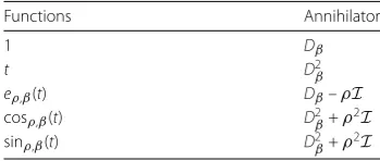
Table1indicates a list of some functions and their annihilators.

Example3.30 Consider the equation

D2βy(t) – 4Dβy(t) + 3y(t) =e5,β(t). (3.52)

Equation (3.52) can be rewritten in the form

(23)

Table 1 A list of some functions and their annihilators

Functions Annihilator

1 Dβ

t D2_β

eρ,β(t) Dβ–ρI

cosρ,β(t) D2β+ρ

2_I

sinρ,β(t) D2_β+ρ2I

Multiplying both sides by the annihilator (Dβ– 5I), we get that ify(t) is a solution of (3.52),

theny(t) satisﬁes

(Dβ– 3I)(Dβ–I)(Dβ– 5I)y(t) = 0.

Hence,

y(t) =c1e3,β(t) +c2e1,β(t) +c3e5,β(t).

One can see thatϕ(t) = (1/8)e5,β(t) is a solution of equation (3.52). Therefore, the general

solution of equation (3.52) has the following form:

y(t) =c1e3,β(t) +c2e1,β(t) + (1/8)e5,β(t).

4 Conclusion

In this paper, the sufficient conditions for the existence and uniqueness of solutions of theβ-Cauchy problem were given. Also, a fundamental set of solutions for the homoge-neous linearβ-difference equations when the coefficientsaj(0≤j≤n) are constants was

constructed. Moreover,β-Wronskian and its properties were introduced. Finally, the un-determined coeﬃcients, the variation of parameters, and the annihilator methods for the non-homogeneous case were presented.

Acknowledgements

The authors sincerely thank the referees for their valuable suggestions and comments.

Funding Not applicable.

Competing interests

The authors declare that they have no competing interests.

Authors’ contributions

All authors contributed equally and signiﬁcantly in writing this article. All authors read and approved the ﬁnal manuscript.

Author details

1_{Department of Mathematics, Faculty of Science, Ain Shams University, Cairo, Egypt.}2_{Department of Mathematics,}

Faculty of Science, Menouﬁa University, Shibin El-Koom, Egypt.

Publisher’s Note

Springer Nature remains neutral with regard to jurisdictional claims in published maps and institutional aﬃliations.

Received: 16 January 2018 Accepted: 18 July 2018

References

(24)

2. Annaby, M.H., Mansour, Z.S.:q-Fractional Calculus and Equations. Springer, Berlin (2012)

3. Askey, R., Wilson, J.: Some basic hypergeometric orthogonal polynomials that generalize the Jacobi polynomials. Mem. Am. Math. Soc.54, 1–55 (1985)

4. Bangerezako, G.: An Introduction toq-Diﬀerence Equations. Bujumbura (2008)

5. Cresson, J., Frederico, G., Torres, D.F.M.: Constants of motion for non-diﬀerentiable quantum variational problems. Topol. Methods Nonlinear Anal.33, 217–231 (2009)

6. Faried, N., Shehata, E.M., El Zafarani, R.M.: On homogeneous second order linear general quantum diﬀerence equations. J. Inequal. Appl.2017, 198 (2017).https://doi.org/10.1186/s13660-017-1471-3

7. Gasper, G., Rahman, M.: Basic Hypergeometric Series. Cambridge University Press, Cambridge (1990) 8. Hamza, A.E., Ahmed, S.M.: Theory of linear Hahn diﬀerence equations. J. Adv. Math.4(2), 441–461 (2013) 9. Hamza, A.E., Sarhan, A.M., Shehata, E.M.: Exponential, trigonometric and hyperbolic functions associated with a

general quantum diﬀerence operator. Adv. Dyn. Syst. Appl.12(1), 25–38 (2017)

10. Hamza, A.E., Sarhan, A.M., Shehata, E.M., Aldowah, K.A.: A general quantum diﬀerence calculus. Adv. Diﬀer. Equ.2015, 182 (2015).https://doi.org/10.1186/s13660-015-0518-3

11. Hamza, A.E., Shehata, E.M.: Existence and uniqueness of solutions of general quantum diﬀerence equations. Adv. Dyn. Syst. Appl.11, 45–58 (2016)

12. Kac, V., Cheung, P.: Quantum Calculus. Springer, New York (2002)

13. Malinowska, A.B., Torres, D.F.M.: Quantum Variational Calculus. Briefs in Electrical and Computer Engineering—Control, Automation and Robotics. Springer, Berlin (2014)