Essays in Modelling and Estimating Value-at-Risk
Yang Yan
A thesis submitted to the Department of Statistics of the London School of Economics for the degree of
Doctor of Philosophy, London
Contents
1 Introduction 6
2 Semi- and nonparametric (G)ARCH Process 9
2.1 Introduction . . . 9
2.2 The GARCH Model . . . 9
2.3 The Univariate Model . . . 10
2.3.1 Error Density . . . 10
2.3.2 Functional form of Volatility Function . . . 11
2.3.3 Relationship between Mean and Variance . . . 14
2.3.4 Long Memory . . . 15
2.3.5 Locally Stationary Processes . . . 16
2.3.6 Continuous Time . . . 16
2.4 The Multivariate Case . . . 17
2.4.1 Error Density . . . 17
2.4.2 Conditional Covariance Matrix . . . 20
2.5 Conclusion . . . 21
3 E¢ cient Estimation of Conditional Risk Measures in a Semiparametric GARCH Model 22 3.1 Introduction . . . 22
3.2 E¢ cient estimation of . . . 25
3.3 E¢ cient estimation ofq andES . . . 29
3.3.1 Quantile estimation with true errors available . . . 29
3.3.2 Quantile estimation with estimated parameters . . . 31
3.5 Numerical Work . . . 35
3.5.1 Simulations . . . 35
3.6 Empirical Work . . . 50
3.6.1 Descriptive Statistics . . . 50
3.6.2 Backtesting VaR . . . 51
3.6.3 Backtesting ES . . . 57
3.7 Conclusion and Extension . . . 61
3.8 Appendix . . . 62
3.8.1 Proofs . . . 62
3.8.2 Second Step Updates by Newton Methods . . . 79
4 Semiparametric Value-at-Risk Forecasts for ARCH(1) Models 81 4.1 Introduction . . . 81
4.2 The model and Value-at-Risk forecasts . . . 82
4.3 Asymptotic theory . . . 86
4.4 Extreme Value Theory . . . 90
4.4.1 Block Maxima . . . 91
4.4.2 Threshold Exceedances . . . 91
4.5 Simulations . . . 95
4.5.1 F(x) :Student-t Distribution . . . 95
4.5.2 F(x): Skewness-t Distribution (Hansen, 1994) . . . 97
4.6 Empirical Study . . . 99
4.6.1 Descriptive Statistics . . . 99
4.6.2 Models . . . 100
4.6.3 Forecasting Performance . . . 101
4.7 Conclusion . . . 112
4.8 Appendix . . . 113
4.8.1 Lemmas . . . 113
Declaration
I certify that the thesis I have presented for examination for the MPhil/PhD degree of the London School of Economics and Political Science is solely my own work other than where I have clearly indicated that it is the work of others (in which case the extent of any work carried out jointly by me and any other person is clearly identi…ed in it).
The copyright of this thesis rests with the author. Quotation from it is permitted, provided that full acknowledgement is made. This thesis may not be reproduced without my prior written consent.I warrant that this authorisation does not, to the best of my belief, infringe the rights of any third party.
Preface
Throughout my 4 year PhD study at LSE, I have received invaluabe encouragement and support from my supervisors, Prof. Oliver Linton and Prof. Qiwei Yao, for which I am very grateful. Oliver has been an inspiring mentor leading me to the world of semiparametric and nonparametric world, and a great personal friend helping me through many di¢ culties. Qiwei has patiently discussed various statistical questions with me and provided helpful ideas along the way. Thanks Prof. Xiao-hong Chen, Prof. Piotr Fryzlewicz and Dr. Matteo Barigozzi for their comments and suggestions about my work.
I would like to thank the faculty and the fellow students in my department, expecially my o¢ cemates, who make my four years’ stay a great experience. Thanks those who organize and attend the Joint Econometrics and Statistics Workshop in LSE and the Econometrics Workshop in the Economics Department, University of Cambridge. Sharing and discussing innovative ideas with them in those occasions are such pleasant moments.
Abstract
Chapter 1
Introduction
The attention placed on e¤ective risk management in the …nancial industry has never been greater, especially after the recent …nancial crisis. The pro…t-driven industry is aware of the importance of measuring and managing risk properly. The Basel Committee (1996) also requires …nancial institutions to hold a certain amount of cash against market risk. Value-at-Risk (VaR), as one of the measures of market risk, becomes widely known when JP morgan introduces Riskmetrics (1996) and set an industry standard. As a forward looking estimate, VaR is de…ned as the maximum potential loss in value of a portfolio of …nancial instruments with a given con…dence level over a certain horizon. It is an important risk measure as portfolio managers are concerned with large potential loss in asset returns.
Consistency and asymptotic normality have been established under various conditions, see Weiss (1986), Lee and Hansen (1994), Hall and Yao (2003), and Jensen and Rahbek (2006). For the semiparametric models, references can be found in Engle and Gonzalez-Rivera (1991) , Linton (1993) and Drost and Klaassen (1997).
In practice, full parametric methods are very popular, but the commonly used normal distribuion is a ‡aw, since most of the …nancial returns have heavy-tails. Fully nonparametric methods,such as Historical Simulation, are easy to implement, but do not provide precise VaR prediction. Semi-parametric method, on the other hand, have been found to perform relatively well. The approach contains a parametric GARCH estimation and a nonparametric standardized residual estimation. It is accurate and at the same time ‡exible, because there are a rich class of GARCH family models to choose and no speci…c distribution assumption is required. The approach has been proposed in Pritsker (1997), Hull and White (1998), McNeil and Frey (2000) and Kuestre, Mittnik and Paolella (2006).
The thesis contributes to the semi- and nonparametric work in VaR modelling. Two general classes of semiparametric models have been proposed. Moment constraints are often used to iden-tify and estimate the mean and variance parameters and are however discarded when estimating error quantiles. In order to prevent this e¢ ciency loss in quantile estimation,the …rst approach is introduced by de…ning some e¢ cient estimators of the risk measures in a semiparametric GARCH model through moment constraints and a quantile estimator based on inverting an empirical likeli-hood weighted distribution. It is found that the new quantile estimator is uniformly more e¢ cient than the simple empirical quantile and a quantile estimator based on normalized residuals. At the same time, the e¢ ciency gain in error quantile estimation hinges on the e¢ ciency of estimators of the variance parameters. We show that the same conclusion applies to the estimation of conditional Expected Shortfall.
The second method is a new method to forecast one-period-ahead Value-at-Risk (VaR) in general ARCH(1) models with possibly heavy-tailed errors. The proposed method is based on least square estimation for the log-transformed model. This method imposes weak moment conditions on the errors. Consequently, it has better prediction performance than commonly used QMLE-based VaR methods in the presence of non-normal errors. In addition, we characterize the asymptotic distribution of the proposed VaR forecast, and this distribution accounts for the uncertainty in volatility estimation.
estimation and testing of the ARCH process, Bauwens, Laurent and Rombouts (2006) talk about multivariate GARCH models, Bollerslev (2009) provides an encyclopedic reference and Terasvirta (2009) summarises univariate GARCH models. However, no one has focused on semi and nonpara-metric approach of estimating ARCH/GARCH process. Chapter 2 of the thesis …lls the needs by surveying the semi- and nonparametric approaches of ARCH/GARCH estimation. Chapter 3 and 4 propose two di¤erent classes of semiparametric approaches of VaR prediction.
Chapter 2
Semi- and nonparametric
(G)ARCH Process
2.1
Introduction
The key properties of …nancial time series appear to be: (a) Marginal distributions have heavy tails and thin centres (Leptokurtosis); (b) the scale or spread appears to change over time; (c) Return series appear to be almost uncorrelated over time but to be dependent through higher moments. See Mandelbrot (1963) and Fama (1965) for some early discussions. The traditional linear models like the autoregressive moving average class do not capture all these phenomena well. This is the motivation for using nonlinear models. This chapter is about the nonparametric approach.
2.2
The GARCH Model
Stochastic volatility models are of considerable current interest in empirical …nance following the seminal work of Engle (1982). Perhaps still the most popular version is Bollerslev’s (1986) GARCH(1,1) model in which the conditional variance 2
t of a martingale di¤erence sequenceytis
2
t =!+ 2t 1+ yt2 1; (2.1)
process arises when
yt t
="t (2.2)
is i.i.d. with mean zero and variance one, where 2
t is de…ned in (2.1). The most common special case is where"tare also standard normal. The semi-strong form arises when for"tin (2.2)
E("tjFt 1) = 0andE("2t 1jFt 1) = 0; (2.3)
where Ft 1 is the sigma …eld generated by the entire past history of they process. Finally, there
is a weak form in which 2
t is de…ned as a projection on a certain subspace, so that the actual conditional variance may not coincide with (2.1). The properties of the strong GARCH process are well understood, and under restrictions on the parameters = (!; ; )it can be shown to be strictly positive with probability one, to be weakly and/or strictly stationary, and to be geometrically mixing and ergodic. The weaknesses of the model are by now well documented, see Tsay (2007) for example.
2.3
The Univariate Model
There are several di¤erent ways in which nonparametric components have been introduced into stochastic volatility models. This work was designed to overcome some of the restrictiveness of the parametric assumptions in Gaussian strong GARCH models.
2.3.1
Error Density
suppose that
yt = "t t
2
t = !+ 2t 1+ y2t 1;
where"tis i.i.d. with densityfof unknown functional form. There is evidence that the density of the standardized residuals "t=yt= t is non-Gaussian. One can obtain more e¢ cient estimates of the parameters of interest by estimating f nonparametrically. Linton (1993) and Drost and Klaassen (1997) developed kernel based estimates and establish the semiparametric e¢ ciency bounds for estimation of the parameters. In some cases, e.g., if f is symmetric about zero, it is possible to adaptively estimate some parameters, i.e., one can achieve the same asymptotic e¢ ciency as if one knew the error density. In other cases, or for some parameters, it is not possible to adapt, i.e., it is not possible to estimate as e¢ ciently as iff were known. These semiparametric models can readily be applied to deliver value at risk and conditional value at risk measures based on the estimated density.
2.3.2
Functional form of Volatility Function
Another line of work has been to question the speci…c functional form of the volatility function, since estimation is not robust with respect to its speci…cation. The news impact curve is the relationship between 2
t andyt 1=y holding past values 2t 1constant at some level 2. This is an important
relationship that describes how new information a¤ects volatility. For the GARCH process, the news impact curve is
m(y; 2) =!+ y2+ 2: (2.4)
It is separable in 2; i.e., @m(y; 2)=@ 2 does not depend on y; it is an even function of news y; i.e.,m(y; 2) =m( y; 2);and it is a quadratic function ofy with minimum at zero:The evenness property implies that cov(y2t; yt j) = 0for"twith distribution symmetric about zero:
Because of limited liability, we might expect that negative and positive shocks have di¤erent e¤ects on the volatility of stock returns, for example. The evenness of the GARCH process news impact curve rules out such ‘leverage e¤ects’. Nelson (1991) introduced the Exponential GARCH model to address this issue. Let ht= log 2t and letht =!+ [ "t 1+ j"t 1j] + ht 1; where
example, cov(y2
t; yt j) 6= 0 even when "t is symmetric about zero. An alternative approach to allowing asymmetric news impact curve is the Glosten, Jeganathan and Runkle (1994) model 2
t = !+ 2
t 1+ y2t 1+ y2t 11(yt 1<0):
There are many di¤erent parametric approaches to modelling the news impact curve and they can give quite di¤erent answers in the range of perhaps most interest to practitioners. This motivates a nonparametric approach, because of the greater ‡exibility in functional form thereby allowed. The nonparametric ARCH literature apparently begins with Pagan and Schwert (1990) and Pagan and Hong (1991). They consider the case where 2
t = 2(yt 1);where ( )is a smooth but unknown
function, and the multilag version 2
t = 2(yt 1; yt 2; : : : ; yt d):This allows for a general shape to the news impact curve and nests all the parametric ARCH processes. Under some general conditions on ( )(for example that ( )does not grow at a more than quadratic rate in the tails) the processy is geometrically strong mixing. Härdle and Tsybakov (1997) applied local linear …t to estimate the volatility function together with the mean function and derived their joint asymptotic properties. The multivariate extension is given in Härdle, Tsybakov and Yang (1996). Masry and Tjøstheim (1995) also estimate nonparametric ARCH models using the Nadaraya-Watson kernel estimator. Lu and Linton (2006) extended the CLT to processes that are only near epoch dependent. Fan and Yao (1998) have discussed e¢ ciency issues in this model, see also Avramidis (2002). Franke, Neumann, and Stockis (2004) have considered the application of bootstrap for improved inference. In practice, it is necessary to include many lagged variables in 2(:)to match the dependence found in …nancial
data. The problem with this is that nonparametric estimation of a multi-dimension regression surface su¤ers from the well-known “curse of dimensionality”: the optimal rate of convergence decreases with dimensionalityd;see Stone (1980). In addition, it is hard to describe, interpret and understand the estimated regression surface when the dimension is more than two. Furthermore, even for largedthis model greatly restricts the dynamics for the variance process since it e¤ectively corresponds to an ARCH(d) model, which is known in the parametric case not to capture the dynamics well. In particular, if the conditional variance is highly persistent, the non-parametric estimator of the conditional variance will provide a poor approximation, as reported in Perron (1998). So not only does this model not capture adequately the time series properties of many datasets, but the statistical properties of the estimators can be poor, and the resulting estimators hard to interpret.
been used in many contexts, see Hastie and Tibshirani (1990). Suppose that
2
t =cv+ d
X
j=1 2
j(yt j) (2.5)
for some unknown functions 2
j: The functions 2j are allowed to be of general functional form but only depend on yt j: This class of processes nests many parametric ARCH models. Again, under growth conditions the process y can be shown to be stationary and geometrically mixing. The functions 2
j can be estimated by special kernel regression techniques, such as the method of marginal integration, see Linton and Nielsen (1995) and Tjøstheim and Auestad (1994). The best achievable rate of convergence for estimates of 2
j(:)is that of one-dimensional nonparametric regression, see Stone (1985). Masry and Tjøstheim (1995) developed estimators for a class of time series models including (2.5). Yang, Härdle, and Nielsen (1999) proposed an alternative nonlinear ARCH model in which the conditional mean is again additive, but the volatility is multiplicative
2
t =cv
Qd
j=1 2j(yt j): Kim and Linton (2004) generalized this model to allow for arbitrary [but known] transformations, i.e.,G( 2
t) =cv+
Pd
j=1 2j(yt j);whereG(:)is a known function like log or level. The typical empirical …ndings are that the news impact curves have an inverted asymmetric U-shape.
These models address the curse of dimensionality but they are rather restrictive with respect to the amount of information allowed to a¤ect volatility, and in particular do not nest the GARCH(1,1) process. Linton and Mammen (2005) proposed the following model
2
t( ; m) =
1
X
j=1
j( )m(yt j); (2.6)
where 2 Rp and m is an unknown but smooth function. The coe¢ cients
j( ) satisfy at least j( ) 0 andP1j=1 j( )<1 for all 2 : A special case of this model is the Engle and Ng (1993) PNP model where
2
t = 2t 1+m(yt j);
denoted AGARCH.
Figure 1: News impact curve (PNP v.s. AGARCH)
Yang (2006) introduced a semiparametric index model
2
t =g
0
@X1
j=1
j(yt j; )
1
A;
where j(y; )are known functions for eachj satisfying some decay condition andgis smooth but unknown. This process nests the GARCH(1,1) whengis the identity, but also the quadratic model considered in Robinson (1991).
Audrino and Bühlmann (2001) proposed their model as 2
t = (yt 1; 2t 1)for some smooth but
unknown function (:);and includes the PNP model as a special case. They proposed an estimation algorithm. However, they did not establish the distribution theory of their estimator, and this may be very di¢ cult to establish due to the generality of the model.
2.3.3
Relationship between Mean and Variance
The above discussion has centered on the evolution of volatility itself, whereas one is often very interested in the mean as well. One might expect that risk and return should be related, Merton (1973). The GARCH-in-Mean process captures this idea, it is
for various functional forms of g e.g., linear and log-linear and for some given speci…cation of 2
t. Engle, Lilien and Robbins (1987) introduced this model and applied it to the study of the term Structure. Here,bare parameters to be estimated along with the parameters of the error variance. Some authors …nd small but signi…cant e¤ects. Again, the nonparametric approach is well motivated here on grounds of ‡exibility. Pagan and Hong (1991) and Pagan and Ullah (1988) considered a case where the conditional variance is nonparametric (with a …nite number of lags) but enters in the mean equation linearly or log linearly. Linton and Perron (2002) studied the case where g is nonparametric but 2
t is parametric, for example GARCH. The estimation algorithm was applied to stock index return data. Their estimated gfunction was non-monotonic for daily S&P500 returns.
2.3.4
Long Memory
Another line of work has argued that conventional models involve a dependence structure that does not …t the data well enough. The GARCH(1,1) process 2
t =!+ 2t 1+ yt2 1 is of the form
2
t =c0+
1
X
j=1
cjy2t j (2.7)
for constants cj satisfying cj = j 1; provided the process is weakly stationary, which requires
+ <1: These coe¢ cients decay very rapidly so the actual amount of memory is quite limited. There is some empirical evidence on the autocorrelation function of y2
t for high frequency returns data that suggests a slower decay rate than would be implied by these coe¢ cients, see Bollerslev and Mikkelson (1996). Long memory models essentially are of the form (2.7) but with slower decay rates. For example, suppose that cj =j for some >0:The coe¢ cients satisfy P1j=1c2
j <1 provided >1=2:Fractional integration (FIGARCH) leads to such an expansion. There is a single parameter calleddthat determines the memory properties of the series, and
(1 L)d 2t =!+ 2t 1("2t 1 1);
where (1 L)d denotes the fractional di¤erencing operator. When d = 1 we have the standard IGARCH model. For d6= 1 we can de…ne the binomial expansion of(1 L) d in the form given above. See Robinson (1991) and Bollerslev and Mikkelson (1996) for models. The evidence for long memory is often based on sample autocovariances of y2
2.3.5
Locally Stationary Processes
Recently, another criticism of GARCH processes has come to the fore, namely their usual assumption of stationarity. The IGARCH process (where + = 1) is one type of nonstationary GARCH model but it has certain undesirable features like the non-existence of the variance. An alternative approach is to model the coe¢ cients of a GARCH process as changing over time, thus
2
t =!(xtT) + (xtT) 2t 1+ (xtT)(yt 1 t 1)2;
where!; ;and are smooth but otherwise unknown functions of a variablextT:WhenxtT =t=T; this class of processes is nonstationary but can be viewed as locally stationary along the lines of Dahlhaus (1997), provided the memory is weak, i.e., ( ) + ( )<1:In this way the unconditional variance exists, i.e., E[ 2t] < 1; but can change slowly over time as can the memory. Dahlhaus and Subba Rao (2006) have recently provided a comprehensive theory of such processes and about inference methods for the ARCH special case. See Spokoiny (2007) for a further review.
Engle and Rangel (2008) propose a special case of this model where the unconditional variance
2(t=T) =!(t=T)=(1 (t=T) (t=T))varies over time but the coe¢ cients (t=T)and (t=T)are
assumed to be constant. In this way, we can writeyt= (t=T)gt1=2"t, wheregtis a unit GARCH(1,1) process representing "high frequency" volatility, while 2(t=T) is the low-frequency unconditional
volatility modelled nonparametrically. Engle and Rangel (2008) also allow for covariates in the low frequency component of volatility.
2.3.6
Continuous Time
2.4
The Multivariate Case
It is important to extend the volatility models to the multivariate framework, as understanding the comovements of di¤erent …nancial returns is also of great interest. The speci…cation of an MGARCH model should be ‡exible enough to represent the dynamics structure of the conditional variances and covariance matrix and parsimonious enough to deal with the rapid expansion of the parameters when the dimension increases. Semiparametric and nonparametric methods o¤er an alternative way to the parametric estimation by taking the advantage of not imposing a particular structure on the data. In general we have a vector time series yt2Rn;that satis…es
yt= 1t=2"t; (2.8)
where "t is a vector of martingale di¤erence sequences satisfying E["tjFt 1] = 0 and E["t">t
InjFt 1] = 0; while t is a symmetric positive de…nite matrix. In this case, tis the conditional
covariance matrix of yt given its own history. The usual approach here is to specify a parametric model for tand perhaps also the marginal density of "t: There are many parametric models for t;and we just mention two recent developments that are particularly useful for large dimensional systems. First, the so-called CCC (constant conditional correlation) (Bollerslev (1990)) models where
t=DtRDt; whereDtis a diagonal matrix with elements it;where 2
itfollows a univariate parametric GARCH or other speci…cation, whileRis annbyncorrelation matrix. The second model generalizes this to allowRto vary with time albeit in a restricted parametric way, and is thereby called DCC (dynamic conditional correlation)(Engle (2002)).
2.4.1
Error Density
methods can often deliver e¢ ciency gains but may not be robust to say dependent or time varying "t. In practice, the estimated density is quite heavy tailed but close to symmetric for stock returns. It is also worth mentioning the SNP (SemiNonParametric) method, which was …rst introduced by Gallant and Tauchen (1989). The fundamental part of the estimating procedure of the conditional density of a stationary multivariate time series relies on the Hermite series expansion, associating with a model selection strategy to determine the appropriate degree of the expansion. The estimator is consistent under some reasonable regularity conditions.
One major issue with the unrestricted semiparametric model is the curse of dimensionality: asn increases the best possible rate at which the error density can be estimated gets worse and worse. In practice, allowing for four or more variables in an unrestricted way is impractical with even enormous sample sizes. This motivates restricted versions of the general model that embody a compromise between ‡exibility of functional form and reasonable small sample properties of estimation methods.
The …rst class of models is the family of spherically symmetric densities in which
f(x) =g(x>x);
where g : R ! R is an unknown but scalar function. This construction avoids the "curse of dimensionality" problem, and can in principle be applied to very high dimensional systems. This class of distributions is important in …nance, since the CAPM is consistent with returns being jointly elliptically symmetric (i.e., spherically symmetric after location and scale transformation), Ingersoll (1984). Hafner and Rombouts (2007) develop estimation methods for parametrically speci…ed t under this assumption.
Another approach is based on copula functions. By Sklar’s theorem, any multivariate distrib-ution can be modelled by the marginal distribdistrib-ution of each individual series and the dependence structure between individual series which is captured by copula functions. A copula itself is a mul-tivariate distribution function with uniform marginals. The joint distribution function of random variablesX andY de…ned asFX;Y(x; y) =C(F(x); G(y)):A bivariate distribution function whose marginals areF( )andG( );andC( ) : [0:1]2!Ris the copula function measures the dependency.
distribution by estimating the univariate marginal distributions nonparametrically and …tting a parametric copula and its circumvention of the "curse of dimensionality". An important class of the SCOMDY models is the semiparametric copula-based multivariate GARCH models, which has the following set up:
yi;t = i;t"i;t
2
i;t = !i+ pi
X
j=1
i;jy2i;t j+ qi
X
j=1
i;j 2i;t j;
where"t= ("1;t; : : : ; "n;t)>is a sequence of i.i.d. random vectors with zero mean and unit variance.
In this case, the conditional covariance matrix of returns is in the class of the CCC models. The key feature of the SCOMDY is the semiparametric form taken by the joint distribution functionF" of"t:
F"("1; : : : ;"n) =C(F";1("1); : : : ; F";n("n); 0); (2.9)
where C( ) is a parametrized copula function depended on unknown 2 Rm, and for i =
1; : : : ; n, F";i( ) is the marginal distribution function of the innovation which is assumed to be continuous but otherwise unspeci…ed. Many examples of combinations have been introduced in the paper, such as { GARCH(1,1),Normal copula} and { GARCH(1,1), Student’s-tcopula}. They also construct simple estimators of the parameters. They establish the large sample properties of the estimator under a misspeci…ed parametric copula, showing that both of the estimators of unknown dynamic parameters and the marginal distribution are still consistent while the estimator of the copula dependence parameter will converge in this case. Chen and Fan (2006b) modelled a univariate version of this class of semiparametric models, but their two-step estimators are veri…ed to be ine¢ cient and even biased if the time series has strong tail dependence in the simulation study of Chen, Wu and Yi (2009). The new paper considers the e¢ cient estimation by using a sieve MLE method which is …rst introduced by Chen, Fan and Tsyrennikov (2006).
Student-t copula for the dependence. Panchenko (2006) also considered a semiparametric copula-based model applied to risk management. Rodriguez (2007) and Okimoto (2007) proposed the regime-switching copula models for pairs of international stock indices. A recent paper by Chollette, Heinei and Valdesogo (2008) estimated the multivariate regime switching model of copula as an extension of the Pelletier (2006) model to non-Gaussian case.
2.4.2
Conditional Covariance Matrix
Hafner, van Dijk and Franses (2005) proposed a semiparametric approach for the conditional co-variance matrix which allows the conditional co-variance to be modelled parametrically by using any choice of univariate GARCH-type models, while the conditional correlation are estimated by non-parametric methods. The conditional covariance matrix tis de…ned as follows:
t=DtRtDt (2.10)
where Dtis parametrically modelled by any choice of univariate GARCH speci…cation, and Rt is treated nonparametrically as an unknown function of a state variablext;thusRt=R(xt)for some unknown matrix function R(:). The functionR(:)is estimated using kernel methods based ont he rescaled residuals from the initial univariate parametric …ts of the GARCH models.
Recently, Hafner and Linton (2009) introduced a multivariate multiplicative volatility model which can be regarded as the multivariate version of the spline-GARCH model of Engle and Rangel (2008). A vector time series yttakes the form:
yt=H(t=T)1=2G1t=2"t (2.11)
where "tis (at least) a strictly stationary unit conditional variance martingale di¤erence sequence. The model allows the slowly varying unconditional variance matrixH( )to be unknown along with the short run dynamics captured throughG( ), which is itself a unit variance multivariate GARCH process, for example the BEKK model
Gt=I AA> BB>+AGt 1A>+But 1u>t 1B>;
where A; B are parameter matrices andut=G1t=2"t:
unconditional components. The total covariance matrix takes the form:
t=DtLDtCRtDCtDtL;
where DLt = diag( Lit); DtC = diag( Cit) and Rt = ijt;(i; j = 1; : : : ; n;)and ( Lit)2 are the local variances,( Cit)2are the conditional variances and ijtdenote the dynamic correlations. Speci…cally,
L
it = Li(t=T);while 2itC follows a parametric unit GARCH type process. As in parametric DCC models one …rst proceeds by estimating the univariate models and then using standardized residuals to estimate the model for Rt:
2.5
Conclusion
Chapter 3
E¢ cient Estimation of Conditional
Risk Measures in a
Semiparametric GARCH Model
3.1
Introduction
Many popular time series models specify some parametric or nonparametric structure for the con-ditional mean and variance. Often, these models are completed by a sequence of i.i.d errors"t.1 For example, many models can be written in the form of T(yt; yt 1; : : :; ) ="t;where the parametric model T( ; )is used to remove the temporal dependence structure inytso that the error"tis i.i.d with certain distributionF( ). Parameters andF( )together de…ne the model. Often one assumes moment conditions on "t such as it being mean zero and variance one. These moment constraints are often used to identify and estimate the mean and variance parameters but are however often discarded when estimating the error distribution or quantile. Knowledge of the conditional distrib-ution is very important in …nance since all …nancial instruments are more or less pricing or hedging certain sections of the distribution of underlying assets. For example, mean-variance trade-o¤ in portfolio management is concerned with the …rst and second moments; exotic derivatives are traded for transferring downside risks, which are lower portions of the asset’s distribution. Other prac-tical usage of conditional distribution estimation includes the risk-neutral density estimation and Value-at-Risk (VaR) estimation.
In this chapter, we consider how best to utilize this conditional information to estimate the distribution F( ), and further the quantiles of"t, so that one can construct an e¢ cient estimator for the conditional distribution and hence quantiles of yt+1 given Ft=fyt; yt 1; : : : ; y0g. Besides
proposing a VaR estimator, we also introduce Expected Shortfall (ES)
Recently, it has been argued that Value at Risk is not a coherent measure of risk, speci…cally it can violate the subadditivity axiom of Artzner et al. (1999). Instead the expected shortfall (ES) is an alternative risk measure that does satisfy all of their axioms. ES is de…ned as the expected return on the portfolio in the worst 100 % of the cases. ES incorporates more information than VaR because ES gives the average loss in the tail below100 %. The estimation of unconditional ES has been considered in Scaillet (2004) and Chen (2008). The recent Basel Committee on Banking Supervision round III has suggested using expected shortfall in place of value at risk, so this measure is likely to gain in prominence in the future.
We consider the following popular AR(p)-GARCH(1,1) model
yt =
p
X
j=1
jyt j+h
1=2
t "t (3.1)
ht = !+ ht 1+ u2t 1;
whereut=h1t=2"t;andf"tgis an i.i.d sequence of innovations with mean zero and variance one and pis a …nite and known integer. We suppose that"thas a density function f( ), which is unknown apart from the two moment conditions:
Z
xf(x)dx= 0; Z
x2f(x)dx= 1: (3.2)
These moment conditions are standard in parametric settings and identify ht as the conditional variance ofytgivenFt 1:Furthermore, the error density and all the parameters are jointly identi…ed
in the semiparametric model. In this case, the conditional Value-at-Risk of yt givenFt 1 and the
conditional expected shortfall of ytgivenFt 1are respectively,
t( ) =
p
X
j=1
jyt j+h1t=2q
t( ) = E[ytjyt t( );Ft 1]
=
p
X
j=1
=
p
X
j=1
jyt j+h1t=2ES ;
whereq is the -quantile of"t;whileES =E["tj"t q ]is the -expected shortfall of"t:In the sequel we assume that p= 0for simplicity of notation. This is quite a common simpli…cation in the literature; the main thrust of our results carry over to the more general pcase.
Let = (!; ; ): The goal of this paper is to estimate the parameters ( ; q ; ES )e¢ ciently and plug in these e¢ cient estimators to obtain the conditional quantile bn;t = h1t=2(b)qb and the conditional expected shortfall bt( ) =h
1=2
t (b)dES .
Since this model involves both …nite dimensional parameters and in…nite dimensional parame-ter f( ), we call it a semiparametric model. This chapter constructs an e¢ cient estimator for both and the 0th quantile of f( ),q , for model (3.1) under moment constraints (3.2). Consequently,
the conditional quantile estimator and conditional expected shortfall estimator are e¢ cient. Estimation of GARCH parameters has a long history. However, there are only limited papers discussing the e¢ ciency issues involved in estimating semiparametric GARCH models. The …rst attempt is due to Engel and GonzalezRivera (1991), who showed partial success in achieving e¢ -ciency via Monte Carlo simulations. In their theoretical work, Linton (1993) and Drost and Klaassen (1997) explained that full adaptive estimation of is not possible and showed their e¢ cient estima-tors for via a reparamerization. Ling and McAleer (2003) further considers adaptive estimation in nonstationary ARMA-GARCH models.
We complement previous work on GARCH models by providing an e¢ cient estimator forF( )
and thus the quantile of"t. It is well known that, in the absence of any auxilliary information about F( ), the empirical distribution functionFb(x) =n 1Pn
of VaR and ES in GARCH models. We show that, the resulting quantile and ES estimators for " are e¢ cient. Furthermore, the conditional VaR t( ) and ES estimators t( ) are asymptotically mixed-normal.
Various quantile estimators have been proposed recently, see Koenker, and Xiao (2009) and Chen, Koenker, and Xiao (2009). For fully nonparametric estimators, see Chen and Tang (2005) and Cai and Wang (2008). However, nonparametric estimators are subject to the curse of dimensionality and thus not widely applicable in practice. Furthermore, these nonparametric quantile estimators are too ‡exible to capture the stylized fact that …nancial returns are conditionally heteroskedastic. Given that this time-varying volatility is the key feature of …nancial time series, historical simulation method would be more advantageous than nonparametric methods in VaR forecasting. In our semiparametric model, the quantile estimator preserves the property of time-varying volatility and allows other aspect of conditional distribution unspeci…ed. Model information is fully explored in the estimation so we gain by providing an e¢ cient solution to conditional quantile estimation. Furthermore, the parametric …lter (the GARCH model for volatility) bundle the conditioning set into a one-dimensional volatility so that there is no curse of dimensionality.
To the best of our knowledge, the only paper to address e¢ cient conditional quantile estimation is Komunjer and Vuong (2010). However, their model is di¤erent from ours: they consider e¢ cient conditional quantile estimation without moment constraints (3.2). Ai and Chen (2003) provide a very general framework for estimation and e¢ ciency in semiparametric time series models de…ned through moment restrictions. No doubt some of our results can be replicated by their methodology using the sieve method.
We apply our method to simulated data and daily stock return data. We …nd superior perfor-mance of our forecasting method over some standard alternatives.
We will discuss e¢ cient estimation of in section 2 and e¢ cient estimation ofq in section 3. Once we collect e¢ cient estimators for these parameters, we can construct the conditional quantile estimator t( )and ES estimator t( )and discuss their asymptotic distribution in section 4. We present our simulation results and empirical applications in section 5. Section 6 concludes with further extensions.
3.2
E¢ cient estimation of
pa-rameters cannot fully capture the potential e¢ ciency gain. Linton (1993) considered the ARCH(p) special case of (3.1) with no mean e¤ect and assumed only that the errors were distributed sym-metrically about zero. In that case, the error density is not jointly identi…ed along with all the parameters, although the identi…ed subvector is adaptively estimable. Drost and Klaassen (1997) consider a general case that allowed for di¤erent identi…cation conditions. They showed that a subvector of the parameters can be adaptively estimated while a remaining parameter cannot be.
We rewrite the volatility model to re‡ect this. Speci…cally, now letht=c2+ac2yt2 1+bht 1:
The …nite dimensional parameter in this model = (c; a; b)>2 R3is to be partitioned into two
parts: (c; >)where = (a; b)> 2B for the reason that only is adaptively estimable, see Linton
(1993) and Drost and Klaassen (1997). As a result, we can rewrite the volatility asht( ) =c2gt(a; b), where gt( ) = 1 +au2
t 1+bgt 1( ).
In the sequel we will use the following notations frequently: moment conditionsR1(") = 1("
q ) , R2(") = "; "2 1 >; the Fisher scale score R3(") = 1 +"f
0(")
f(") of the error density f;
derivatives Gt( ) =@loggt( )=@ , G( ) =E[Gt( )],Ht( ) =@loght( )=@ ; H( ) =E[Ht( )],
G2( ) =E
@loggt( ) @
@loggt( )
@ > ; H2( ) =E
@loght( ) @
@loght( ) @ > :
When the argument is evaluated at the true value, we use abbreviation: for example, G=G( 0)
andHt=Ht( 0).
The log-likelihood of observationsfy1; : : : ; yng (givenh0)assuming thatf is known is
L( ) =
n
X
t=1
logf(c 1gt1=2( )yt) + logc 1gt1=2( ):
Then the score function in the parametric model at time tas
lt( ) =
1
2 1 +"t( )
f0("
t( )) f("t( ))
@loght( )
@ :
We now consider the semiparametric model wheref is unknown. To see why the parameter is not adaptively estimable, we consider the density function f(x; ) with a shape parameter 2 . It is clear from E[@lt( ; )=@ ] 6= 0 that the estimation of a¤ects the e¢ ciency of the estimates of . If we knew the density function f( ) and are interested in estimating in presence of the nuisance parameterc, the e¢ cient score function for is the vector
l1t( ) = 1
according to the Convolution Theorem 2.2 in Drost and Klaassen (1997). The density functionf( )
is unknown. Drost and Klaassen (1997) showed that introduction of unknown f( )in presence of unknownc does not change the e¢ cient in‡uence function for .
We make the following assumptions:
Assumptions A
A1. c >0; a 0 andb 0. E[lnfb+ac2"2
tg]<0:
A2. The density function f satis…es the moment restrictions: Rxf(x)dx= 0andRx2f(x)dx= 1;
it has …nite fourth momentRx4f(x)dx <1, and E"4 1 (E"3)26= 0: A3. The density function f is positive and f0 is absolutely continuous with
jjfjj1= sup
x2R
f(x)<1;sup
x2Rj
xjf(x)<1;
Z
jxjf(x)dx <1:
A4. The density function f has positive and …nite Fisher information for scale
0<
Z
(1 +xf0(x)=f(x))2f(x)dx <1:
A5. The density function f for the initial value h01 satis…es that, the likelihood ratio forh01;
ln(h01) = logffen=f n(h01)
Pn
! 0; as n! 1
where the contiguous parameter sequencesen and nare de…ned as in Drost and Klaassen (1997, p199).
Remark. Assumption A.1 ensures the positivity ofht and the strict stationarity ofyt. Since
E[lnfb+ac2"2
tg] b+ac2 1, a su¢ cient condition for strict stationarity isb+ac2<1, see Nelson (1990). A.2 is introduced to make sure that the variance matrixE[R2(")R2(")>]is invertible A.3 is
made because we will need some boundedness off to make a uniform expansion for the empirical distributions, see section 3. A.4 is typically assumed for e¢ ciency discussion, see for example, Linton (1993) and Drost and Klaassen (1997). A.5 is assumed to obtain the uniform LAN theorem and the Convolution Theorem, as in Drost and Klaassen (1997).
discussion of Gaussian QMLE, and Weiss (1986) for OLS. Jensen and Rahbek (2004) considered the asymptotic theory of QMLE for nonstationary GARCH models. We have the following result which extends Drost and Klaassen (1997) and Drost, Klaassen, and Werker (1997).
Theorem 1 Suppose that assumptions A hold. Then there exists an e¢ cient estimatorb that has the following expansion
p
n(b 0) =
1 p n n X t=1
t( 0) +op(1); (3.4)
t( 0) =
0 B @
1
2E[l1tl1t>] 1fGt Gg 0 c0
4G>E[l1tl1t>] 1fGt Gg c20( E"3;1)
1 C A
0 B @ R3("t)
R2("t)
1 C
A:
Consequently,
p
n(b 0) =)N(0; );
= 0 B
@ E[l1tl
>
1t] 1 c20E[l1tl1t>] 1G c0
2G>E[l1tl1>t] 1 c2
0
4fE"
4 1 (E"3)2+G>E[l
1tl1t>] 1Gg
1 C
A:
For technical reasons, the estimator employed in the theorem makes use of sample splitting, discretization, and trimming in order to facilitate the proof. In practice, none of these devices may be desirable.
We have found the following estimator scheme works well in practice. Suppose that k( ) is a symmetric, second-order kernel function with Rk(x)dx= 1and Rxk(x)dx= 0;and lethandbbe positive bandwidths that (in the theory will satisfyh!0; nh4! 1,b!0; nb4! 1):
Estimation Algorithm
1. Letb1= (b
>
1;bc1)>be an initial
p
T-consistent estimator, for example the QMLE, and compute the residualsb"1t=yt=ht1=2(b1):
2. Update the estimator of by using the Newton–Raphson method:
b=b1+ 1
n
Xn
t=1bl1t(b1)bl1t(b1)
>
1
1
n
Xn
t=1bl1t(b1)
bl1t(b1) = 1
2 Gt(b1)
1
n
Xn
s=1Gs(b1) Rb3(b"1t); Rb3(x) = 1 +xfb
0(x)=fb(x)
b
f(x) = 1
nh
Xn
t=1k
b"1t x
h ; fb0(x) =
1
nb2
Xn
t=1k
0 b"1t x
3. Denotebet=ytgt1=2(b)and the e¢ cient estimator for cis
b
c= s
1
n
Xn
t=1be 2
t
1
n
Pn
t=1be3t
Pn
t=1be2t
Xn
t=1bet:
This procedure can be repeated until some convergence criterion is met, although for most theoretical purposes, one iteration is su¢ cient.
Remark. It can be shown that the simpler estimator ec =
q
1
n
Pn
t=1be2t has an asymptotic variance c2
0fE"4 1 +G>E[l1tl1>t] 1Gg=4, which is strictly larger than our e¢ cient estimator bc unless the error distribution is symmetric, i.e. E"3= 0.
3.3
E¢ cient estimation of
q
and
ES
We now turn to the estimation of the quantities of interest. To motivate our theory, we …rst discuss the estimation ofq with the availability of true errors, and then discuss what to do in the case of estimation errors.
3.3.1
Quantile estimation with true errors available
In this subsection we estimate the quantile by inverting various distribution estimators. Because the unknown error distribution satis…es condition (3.2), it is desirable to construct distribution estimators that have this property.
The empirical distribution functionFb(x) =n 1Pn
t=11("t x)is commonly used but it does not impose these moment constraints. In practice, a common approach is to recenter the errors. There-fore, we also consider a modi…ed empirical distribution, FNb (x) = n 1Pn
t=11(("t b")=b" x); whereb"=n 1
Pn
t=1"tandb 2
"=n 1
Pn
t=1"2t (n 1
Pn
t=1"t)2. By construction, this distribution
estimator satis…es the moment constraints (3.2). It is easy to see that the relationship between
b
F(x)andFNb (x)isFNb (x) =Fb(b"+xb").
In this paper, we consider a new weighted empirical distribution estimatorFwb (x) =Pnt=1wtb1("t x), where the empirical likelihood weightsfwbtg come from the following:
max
fwtg
n t=1wt s.t. Xn
t=1wt = 1;
Xn
t=1wt"t= 0;
Xn
t=1wt(" 2
t 1) = 0:
In the absence of the moment constraints, it is easy to see thatarg maxfwtgf
n
t=1wt+ (1
Pn
t=1wt)g= 1=n. In this case our weighted empirical distribution estimator is the same as Fb(x).
Since the unknown distribution is in the family P = ff(x) : Rxf(x)dx = 0;R(x2 1)f(x)dx =
0g; we expect Fwb (x) to be more e¢ cient by incorporating these moment constraints, Bickel, Klaassen, Ritov, and Wellner (1993). Lemma 1 (appendix) which shows the uniform expansion for the distribution estimators Fb(x);FNb (x)andFwb con…rms our conjecture. It is well-known that
pn(Fb(x) F(x)) =
) N(0; F(x)(1 F(x))). The empirical distribution is the most e¢ cient es-timator without any auxiliary information about F( ). This is consistent with our result because wt= 1=nis the solution to the problem of maxfwtgf
n
t=1wt+ (1
Pn
t=1wt)g.
We obtain an asymptotic expansion forFbN(x)andFbw(x)in the appendix (Lemma 1) and show that:
p
n(FNb (x) F(x)) =) N(0; F(x)(1 F(x)) +Cx)
p
n(Fbw(x) F(x)) =) N(0; F(x)(1 F(x)) A>xB 1Ax):
We can see that normalization has introduced some additional error; see Durbin (1973). This estimation error has been cumulated and is re‡ected by the additional term Cx in the asymptotic variance. The sign of Cx function is indeterminate, see the Figure 1 in the appendix. It depends on the density f(x)and the point to be evaluated. For standard normal distribution and student distributions,Cx 0, which means, for these two distributions,FNb (x)is more e¢ cient than Fb(x). In contrast, for mixed normal distribution and Chi-squared distributions, the e¢ ciency ranking depends on the point to be evaluated. On the other hand, weighting the empirical distribution takes into account the information in (3.2), which is re‡ected in the term A>
xB 1Ax. This term can be explained as the projection of 1(" x) F(x) ontoR2("). The covariance Ax measures the relevance of moment constraints (3.2) in estimating the distribution function. The information content that helps in estimating unknown F(x)is weak when Ax is small. In case of Ax= 0, the moment constraints (3.2) do not have any explanation power at all since1(" x) F(x)andR2(")
is orthogonal. In the appendix we give conditions under whichFNb (x)andFb(x)can be as e¢ cient as Fwb (x).
We now de…ne our quantile and expected shortfall estimators. For an estimated c.d.f.,F ;e let
e
q = supft:Fe(t) g=Fe 1( ) ; ESg = 1
Z qe
1
b1 =q ;b b2 =qbN ;b3 =qbw ;b4 =dES ;b5 =dESN ; andb6 =dESw be de…ned from (3.5) using theFb(x);FNb (x);andFwb (x)as required:The next theorem presents the asymptotic distribution of these quantile estimators. De…ne:
V1 =
(1 )
f(q )2 ; V2=
(1 )
f(q )2 +
Cq
f(q )2 ; V3=
(1 )
f(q )2
A>q B 1A
q f(q )2
V4 = 2var((" q )1(" q )) ; V5= 2var((" q )1(" q ) "
"2
2
Z q
1
xf(x)dx))
V6 = 2var((" q )1(" q ) +R>2(")B 1
Z q
1
Axdx):
Theorem 2 Suppose that assumptions A.1-A.5 hold. The quantile and expected shortfall estima-tors are asymptotically normal
p
n(bj j) =)N(0; Vj)
forj= 1; : : : ;6; where 1= 2= 3=q and 4= 5= 6=ES .
Remark. It is clear from the comparison of asymptotic variances thatqbw , which is based on
inverting empirically weighted distribution estimators, is the most e¢ cient one. The same conclusion holds for ES since ES is the aggregation of lower quantiles: ESg = 1Rqe1xdFe(x) = 1R0 q de .
Remark. For improvement in mean squared e¢ ciency, one could consider inverting the smoothed
weighted empirical distributionFswb (x) =Pnt=1wtKb (x "t
h )with Fsb(x) =n 1
Pn
t=1K(x "ht)being a special case. However, the …rst order large sample properties will be the same as the unsmoothed one here. The unsmoothed distribution estimators considered in this paper are free from the com-plication of bandwidth choice.
3.3.2
Quantile estimation with estimated parameters
We now assume that we don’t know the true parameters , and so we don’t observe "t. Instead we observe the polluted error, "t( n) =yt=ht1=2( n); where n is an estimator sequence satisfying n 0 =Op(n 1=2). Now we construct an e¢ cient estimator for residual distributionF(x)and
then invert to get back the quantile estimatorqn =Fn1( ). We treat a general class of estimators n for completeness.
Motivated by the e¢ ciency gain shown in Lemma 1, we estimate the quantile by inverting the following distribution function estimator:
bb
Fw(x) = n
X
t=1
bb
where fwbbtg are de…ned by the solution of the following optimization problem
max
fwtg
n t=1wt
s.t. Xn
t=1wt = 1;
Xn
t=1wt"t( n) = 0;
Xn
t=1wt(" 2
t( n) 1) = 0:
For comparison purposes, we also consider the residual empirical distribution estimatorFbb(x) =
n 1Pnt=11("t( n) x)and the standardized empirical distributionFNbb (x) =n 1Pnt=11(("t( n)
bb")=bb" x), where bb"=n 1
Pn
t=1"t( n)and bb
2
"=n 1
Pn
t=1"2t( n) (n 1
Pn
t=1"t( n))2. Suppose that there is an estimatorethat has in‡uence function t( 0), i.e.
p
n(e 0) =
1
p
n n
X
t=1
t( 0) +op(1): (3.7)
In the appendix (Lemma 2 and Corollary 3) we derive uniform expansion of the distribution esti-mators Fbb(x);FbbN(x)andFbbw(x)based oneand give their asymptotic variances, which depend on the in‡uence function t( 0). We next explore these asymptotic variances for some widely used
estimators (with expansion 3.7). Suppose that
t( 0) =Jt( 0)("2t 1); (3.8)
where Jt( 0)2 Ft 1;so that t( 0)is a martingale di¤erence sequence. DenoteJ( 0) =E[Jt( 0)]:
Then the asymptotic variances of the three distribution estimators are respectively:
1;J(x) = F(x)(1 F(x)) +
[E["4] 1]x2f(x)2
4 fH( 0)
>
J( 0)g2+xf(x)H( 0)
>
J( 0)a2(x)
2;J(x) = F(x)(1 F(x)) +
[E["4] 1]x2f(x)2
4 fH( 0)
>
J( 0)g2+xf(x)H( 0)
>
J( 0)a2(x)
+f(x)2+x
2f(x)2[E["4] 1]
4 +xf(x)
2E["3] +xf(x)a
2(x) + 2f(x)a1(x)
+xf(x)2E["3]H( 0)
>
J( 0) +
x2f(x)2[E["4] 1]
2 H( 0)
>
J( 0) 3;J(x) = F(x)(1 F(x)) A>xB 1Ax
+fE["4] 1g xf(x)
2 + 0 1 B
1A
x
2
fH( 0)
>
J( 0)g2:
In the special case of the least squares estimator,
t( 0) =H1( 0) 1ht( 0)
@ht( 0)
@ ("
2
whereH1( 0) =E[@h@t(0)@ht( 0)
@ > ]. DenoteH3( 0) =E[ht( 0) @ht(0)
@ ], thenJt( 0) =H1( 0)
1H 3t( 0):
In the special case of the Gaussian QMLE,
t( 0) =fH2( 0)g 1
1
ht( 0)
@ht( 0)
@ ("
2
t 1);
thenJt( 0) =H2( 0) 1Ht( 0):In both cases the asymptotic variance is increased relative to Lemma
1. Since the QMLE residuals"t(e)are obtained under the moment conditionn 1Pnt=1[Ht(e)("2t(e)
1)] = 0 with probability one, the …rst moment ofFbb(x)isR xdFbb(x) =n 1Pn
t=1("2t(e) 1); which may not be zero with probability one.
We construct quantile estimators by inverting these distribution estimators. Based on the ymptotic expansion of the distribution estimators in the appendix (Lemma 2), we obtain the as-ymptotic properties of the Value at Risk and Expected shortfall estimators, which is the main result of the paper. Let bb1 =bbq ;bb2 =bbqN ;bb3 =bbqw ;bb4 = ddES ;bb5 = ESNdd ; and bb6 = ddESw
be de…ned from (3.5) using the estimated c.d.f.s Fbb(x);FbbN(x);and Fwbb (x)as required (and de…ne correspondingly, 1 = 2 = 3=q and 4 = 5= 6 =ES .): De…ne the asymptotic covariance
matrices:
1 = =
(1 )
f(q )2 +
q2
4 [E"
4 1 (E"3)2] +q (a2q a1q E"3) f(q )
2 = N =
(1 )
f(q )2 +
Cq f(q )2 +
3q2[E"4 1 (E"3)2]
4 +
q (a2q a1q E"3) f(q )
3 = w =
(1 )
f(q )2
A>q B 1Aq
f(q )2 + [
q
2 +
0 1 B 1Aq
f(q ) ]
2[E"4 1 (E"3)2]
4 = ES= 2var (" q )1(" q )
"2 "E"3
2
Z q
1
xf(x)dx
5 = ESN = 2var (" q )1(" q ) "
Z q
1
[f(x) xf(x)
2 E"
3]dx "2
Z q
1
xf(x)dx
6 = ESW = 2var (" q )1(" q ) ("2 "E"3)
Z q
1
[xf(x)
2 + 0 1 B
1Ax]dx
+R>2(")B 1
Z q
1
Axdx :
Theorem 3 Suppose that assumptions A.1-A.5 hold. The quantile and expected shortfall estimators are asymptotically normal:
p
n(bbj j) =)N(0; j)
forj= 1; : : : ;6:
estimators, we can see thatbbqw is more e¢ cient thanbbq . The same conclusion holds for ES.
Remark. Notice that the asymptotic variances of VaRs and ESs do not contain any functional
form of the heteroskedasticity. This is due to the orthogonality in information between estimators for the distributionF(x)and variance estimator for .
Remark. We can compute consistent standard errors by the obvious plug-in method.
3.4
E¢ cient estimation of conditional VaR and conditional
expected shortfall
We have discussed the asymptotic property of e¢ cient estimators b andbbqw . They are shown to be the best among competitors in terms of smallest asymptotic variances. Both are important ingredients to the conditional quantile estimator bn;t as bn;t = h
1=2
t (b)bbqw and the conditional expected shortfall bn;t =h
1=2
t (b)ddESw . In this section, we will show that these two quantities are asymptotically mixed normal. De…ne:
! t=ht( 0)
q2
4 (G
>
t G)E[l1tl1t
>
] 1(Gt G) + w ;
! t=ht( 0)
(
ES2
4 H
>
t Ht+ES
( E"3;1)E ("t q )1("t q ) +R>
2("t)C R2("t)
+ ESW
)
C=
Z q
1
[xf(x)
2 + 0 1 B
1Ax]dx(E"3; 1) +
Z q
1
A>xdxB 1:
Theorem 4 Suppose assumptions A.1-A.5 hold. The conditional quantile estimator bn;t and con-ditional quantile estimator bn;t are asymptotically mixed normal
p
n(bn;t t) =) M N(0; ! t)
p
n(bn;t t) =) M N(0; ! t);
where the random positive scalars ! t and! t are independent of the underlying normals.
Remark. From the in‡uence functions of(ba;bb)andbbqw , we can see that they are asymptotically
orthogonal. This is anticipated as the parameter (a; b)is adaptively estimated with respect to the error distribution.
Remark. This mixed normal distribution asymptotics is similar to results obtained in
see also Hall and Heyde (1980). It follows that pn(bn;t t)=!1t=2 =) N(0;1) and pn(bn;t
t)=!b
1=2
t =)N(0;1);where!b tis a consistent estimator of ! t:Therefore, one can conduct infer-ence about n;t with the usual con…dence intervals.
3.5
Numerical Work
In this section we present some numerical evidence. The …rst part is Monte-Carlo simulation and the second is an empirical application.
3.5.1
Simulations
We follow Drost and Klaassen (1997) to simulate several GARCH (1,1) series from the model (1) with the following parameterizations:
1. (c; a; b)2 f(1;0:3;0:6);(1;0:1;0:8);(1;0:05;0:9)g;
2. f(x)2 fN(0;1); M N(2; 2); L; t(5); t(7); t(9); 2
6; 212g;which are, respectively, referred to the
densities of standardized (mean 0 and variance 1) distributions from Normal, Mixed Normal with means (2; 2), Laplace, student distributions with degree of freedom 5, 7 and 9 and chi-squared distribution with 6 and 12 degrees of freedom.
Sample size is set to n = 500;1000. Simulations are carried out 2500 times. We consider the performance of the three distribution estimators and their associated quantile and ES estimators with being 5% and1%. We also have the simulation results for small samples n = 25;50;100, and for IGARCH models with a+b= 1. These results are similar to those in this paper and are available upon request.
The criterion for distribution estimatorFb(x)is the integrated mean squared error (IMSE)
IM SE= Z
E[Fb(x) F(x)]2dx
and that for quantile and ES estimators (bq anddES ) is the mean squared error
M SE=E[(qb q )2];M SE =E[(dES ES )2]:
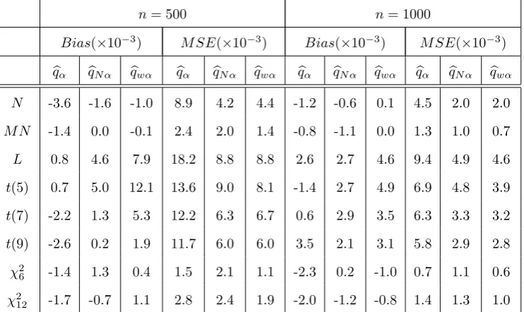
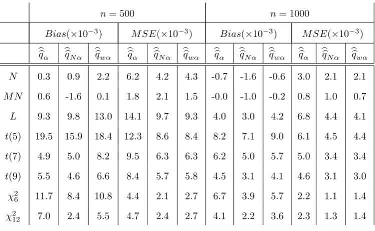
unweighted empirical distribution Fb(x) is very large: it ranged from 50% in case of errors being Laplacian to 72% in the case of Mixed-normal. Figure 2 visualizes this gain by plotting the overlays of simulated distribution estimators with 100 replications. The colored region represents the possible paths of function estimators and it is clear that the magenta area (realizations ofFwb (x)) is has the smaller width than blue area (realizations of Fb(x)). In order to compare the quantile estimators based on inverting these distribution estimators, we compute their average biases and mean squared errors under di¤erent distributional assumptions and in 500 and 1000 sample sizes. The average is taken over 2500 simulations. It is found that qbw performs much better than bq in all cases. This improvement is clearer in the case of = 0:05than the case of = 0:01. This is because the further to the tail ( when ais smaller), the smaller the covariance betweenR2(")and1(" x) .
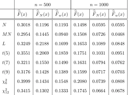
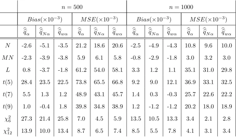
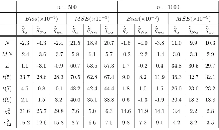
Next, we compare the distribution estimators when the errors are not observable and we use estimated errors from QMLE. Since QMLE is consistent in all above error distribution assumptions, we expect the QMLE residuals will behave close to the true errors, although with some estimation noises. Table 4-6 list the IMSE for distribution estimators under three di¤erent parameterizations. We …nd that, there are e¢ ciency gains by weighting the empirical distribution estimator with empirical likelihoods. Figure 3 visualizes these gains, which vary across the assumptions of true error distributions. Table 7-12 compare the performance of residual quantile estimators. The conclusion is the same: empirical likelihood weighting reduces the variation of quantile estimators. However, these reductions are not of the same magnitude as in i.i.d case. The reason is because we use estimated errors in stead of true errors and the added estimation noise a¤ect the performance of residual based estimators.
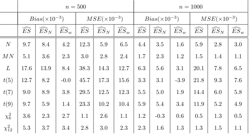
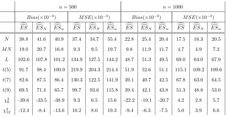
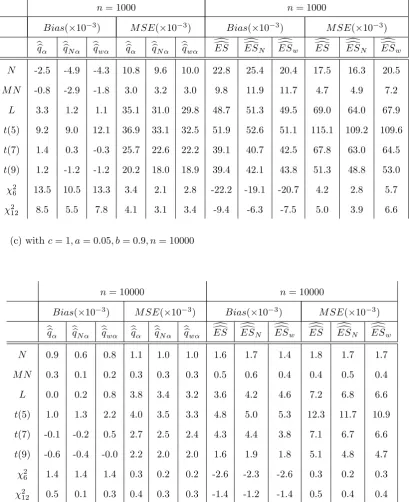
Thirdly, we compare di¤erent estimators for expected shortfall in the case of iid errors and GARCH residuals. As seen from table 15-18, the same conclusion holds for ES. For sample size n=500 and 1000, the proposed estimator does not do very well in the case of a = 0:01, see table 18. This is expected because our e¢ cient estimator (EL-weighted) involves an additional layer of numerical optimization, and for such low quantile/ES, the e¤ective sample size isn=100. Therefore we tabulate the results for large samplen= 10000,which is the table 19(c). It’s clear from table that our proposed VaR and ES estimators outperform other estimators in terms of smaller MSE.(The comparison of the estimators forqb0:01 andESd0:01,when the true errors are available andbbq0:01and
d d
ES0:01, when the polluted errors are calculated are provided in table 19(a) and 19(b)).
Finally, we consider the case of distribution and quantile estimation based on e¢ cient residuals: the estimated errors are residuals from e¢ cient estimation of parameter 0. As we notice that the
only report the results in the case ofc= 1; a= 0:05; b= 0:9. Table 13 summarizes the performance of quantile estimators forq0:01andq0:05, while table 14 reports the true VaR and ES for distribution
estimators and Figure 4 visualize the e¢ ciency gains.
Table 1. Integrated Mean Squared Error ( 10 3) of Distribution Function Estimators
n= 500 n= 1000
b
F(x) FNb (x) Fwb (x) Fb(x) FNb (x) Fwb (x)
N 0.3365 0.1199 0.1212 0.1616 0.0580 0.0583 M N 0.3286 0.1412 0.0916 0.1622 0.0687 0.0462 L 0.3313 0.2188 0.1603 0.1692 0.1092 0.0810 t(5) 0.3419 0.2157 0.1635 0.1657 0.1055 0.0797 t(7) 0.3255 0.1594 0.1458 0.1695 0.0791 0.0708 t(9) 0.3336 0.1439 0.1361 0.1664 0.0730 0.0687
2
6 0.3308 0.1479 0.1217 0.1692 0.0721 0.0605 2
12 0.3297 0.1335 0.1213 0.1692 0.0654 0.0595
Table 2. Comparison of quantile estimators forq0:01 (true errors are available)
n= 500 n= 1000
Bias( 10 3) M SE( 10 3) Bias( 10 3) M SE( 10 3)
b
q qNb qwb qb qNb qwb qb qNb bqw bq qNb qwb
N -2.1 -0.8 3.7 27.1 19.4 22.2 -0.7 -1.1 0.6 14.1 9.9 11.1 M N -1.8 -2.5 -0.5 6.3 5.8 5.6 -1.3 -0.9 -0.4 3.3 3.1 2.9
L -3.7 3.3 17.9 94.3 60.9 68.6 11.9 9.4 11.8 47.8 31.6 31.9 t(5) 25.1 25.3 40.7 102.5 67.5 72.8 8.4 11.4 22.2 50.4 34.1 35.1 t(7) 8.4 10.5 21.1 65.4 45.3 50.9 -1.7 0.1 4.9 34.9 23.1 23.6 t(9) 10.5 9.3 15.4 56.1 36.7 41.8 11.4 8.1 8.9 30.9 20.0 21.3
2
6 -3.4 0.4 -1.7 1.7 3.7 1.7 -1.0 0.5 -0.4 0.9 1.8 0.8 2
Table 3. Comparison of quantile estimators forq0:05 (true errors are available)
n= 500 n= 1000
Bias( 10 3) M SE( 10 3) Bias( 10 3) M SE( 10 3) b
q qbN qbw qb qbN bqw qb bqN qbw qb bqN qbw N -3.6 -1.6 -1.0 8.9 4.2 4.4 -1.2 -0.6 0.1 4.5 2.0 2.0 M N -1.4 0.0 -0.1 2.4 2.0 1.4 -0.8 -1.1 0.0 1.3 1.0 0.7 L 0.8 4.6 7.9 18.2 8.8 8.8 2.6 2.7 4.6 9.4 4.9 4.6 t(5) 0.7 5.0 12.1 13.6 9.0 8.1 -1.4 2.7 4.9 6.9 4.8 3.9 t(7) -2.2 1.3 5.3 12.2 6.3 6.7 0.6 2.9 3.5 6.3 3.3 3.2 t(9) -2.6 0.2 1.9 11.7 6.0 6.0 3.5 2.1 3.1 5.8 2.9 2.8
2
6 -1.4 1.3 0.4 1.5 2.1 1.1 -2.3 0.2 -1.0 0.7 1.1 0.6 2
Table 4. Integrated Mean Squared Error ( 10 3),c= 1; a= 0:3; b= 0:6:
n= 500 n= 1000
bb
F(x) FbbN(x) Fbbw(x) Fbb(x) FbbN(x) Fbbw(x) N 0.3018 0.1196 0.1193 0.1498 0.0595 0.0595 M N 0.2954 0.1445 0.0940 0.1508 0.0726 0.0468 L 0.3249 0.2188 0.1699 0.1653 0.1089 0.0848 t(5) 0.3551 0.2069 0.1859 0.1751 0.1031 0.0951 t(7) 0.3211 0.1550 0.1490 0.1631 0.0794 0.0762 t(9) 0.3176 0.1428 0.1389 0.1599 0.0717 0.0703
2
6 0.3999 0.1434 0.1548 0.2080 0.0739 0.0808 2
12 0.3415 0.1302 0.1333 0.1745 0.0664 0.0678
Table 5. Integrated Mean Squared Error ( 10 3),c= 1; a= 0:1; b= 0:8:
n= 500 n= 1000
bb
F(x) FbbN(x) Fbbw(x) Fbb(x) FbbN(x) Fbbw(x) N 0.3023 0.1195 0.1193 0.1499 0.0594 0.0595 M N 0.2960 0.1442 0.0937 0.1511 0.0726 0.0468 L 0.3250 0.2185 0.1700 0.1655 0.1088 0.0848 t(5) 0.3591 0.2067 0.1891 0.1763 0.1029 0.0962 t(7) 0.3222 0.1550 0.1495 0.1635 0.0792 0.0764 t(9) 0.3187 0.1428 0.1396 0.1600 0.0715 0.0702
2
6 0.4014 0.1430 0.1547 0.2076 0.0738 0.0807 2
12 0.3422 0.1301 0.1335 0.1740 0.0663 0.0672
n= 500 n= 1000 bb
F(x) FbbN(x) Fbbw(x) Fbb(x) FbbN(x) Fbbw(x) N 0.3026 0.1193 0.1191 0.1500 0.0594 0.0595 M N 0.2964 0.1440 0.0937 0.1511 0.0727 0.0468 L 0.3255 0.2182 0.1700 0.1656 0.1088 0.0848 t(5) 0.3607 0.2069 0.1902 0.1769 0.1034 0.0968 t(7) 0.3232 0.1557 0.1502 0.1636 0.0791 0.0763 t(9) 0.3187 0.1428 0.1393 0.1602 0.0715 0.0702
2
6 0.4021 0.1425 0.1548 0.2079 0.0737 0.0808 2
Table 7. Comparison of quantile estimators forq0:01, withc= 1; a= 0:05; b= 0:9
n= 500 n= 1000
Bias( 10 3) M SE( 10 3) Bias( 10 3) M SE( 10 3)
bb
q bbqN bbqw bbq bbqN bbqw bbq bbqN bbqw bbq bbqN bbqw N -2.6 -5.1 -3.5 21.2 18.6 20.6 -2.5 -4.9 -4.3 10.8 9.6 10.0 M N -2.3 -3.9 -3.8 5.9 6.1 5.8 -0.8 -2.9 -1.8 3.0 3.2 3.0
L 0.8 -3.7 -1.8 61.2 54.0 58.1 3.3 1.2 1.1 35.1 31.0 29.8 t(5) 28.4 23.5 22.5 73.8 65.5 66.8 9.2 9.0 12.1 36.9 33.1 32.5 t(7) 5.5 1.3 1.2 48.9 43.1 45.7 1.4 0.3 -0.3 25.7 22.6 22.2 t(9) 1.0 -0.4 1.8 39.8 34.8 38.9 1.2 -1.2 -1.2 20.2 18.0 18.9
2
6 27.3 21.4 25.8 7.0 4.5 5.9 13.5 10.5 13.3 3.4 2.1 2.8 2
Table 8. Comparison of quantile estimators forq0:01, withc= 1; a= 0:3; b= 0:6
n= 500 n= 1000
Bias( 10 3) M SE( 10 3) Bias( 10 3) M SE( 10 3)
bb
q bbqN bbqw bbq bbqN bbqw bbq bbqN bbqw bbq bbqN bbqw N -2.3 -4.3 -2.4 21.5 18.9 20.7 -1.6 -4.0 -3.8 11.0 9.9 10.3 M N -2.4 -3.6 -3.7 5.8 6.1 5.7 -0.2 -2.2 -1.4 3.0 3.3 2.9
L 1.1 -3.1 -0.9 60.7 53.5 57.3 1.7 -0.2 0.4 34.8 30.5 29.7 t(5) 33.7 28.6 28.3 70.5 62.8 67.4 9.0 8.2 11.9 36.3 32.7 32.1 t(7) 4.5 0.8 -0.1 48.2 42.4 44.4 1.8 1.0 1.5 26.0 23.0 23.2 t(9) 2.1 1.5 3.2 40.0 35.1 38.8 0.6 -1.3 -1.9 20.4 18.2 18.8
2
6 31.6 25.7 29.8 7.6 5.0 6.3 14.6 11.9 14.1 3.4 2.2 2.8 2
[image:43.595.106.491.115.343.2]12 16.2 12.6 15.8 8.7 6.6 7.5 9.8 7.2 9.1 4.2 3.2 3.5
Table 9. Comparison of quantile estimators forq0:01, withc= 1; a= 0:1; b= 0:8
n= 500 n= 1000
Bias( 10 3) M SE( 10 3) Bias( 10 3) M SE( 10 3)
bb
q bbqN bbqw bbq bbqN bbqw bbq bbqN bbqw bbq bbqN bbqw N -3.1 -5.5 -3.6 21.4 18.9 20.5 -3.1 -4.0 -2.2 11.2 10.1 10.5 M N -2.5 -4.0 -3.9 5.8 6.0 5.7 -1.5 -3.2 -2.1 2.9 3.2 2.8
L -0.0 -3.8 -0.8 60.8 53.6 58.0 -0.9 -1.2 2.3 37.0 33.1 33.0 t(5) 29.7 25.7 22.1 71.7 64.0 67.4 9.2 9.1 14.0 37.0 33.3 34.4 t(7) 4.3 0.7 -0.1 48.4 42.7 45.4 4.7 3.6 4.9 26.4 23.5 23.3 t(9) 0.7 -0.1 2.3 39.9 35.0 38.4 3.3 1.1 1.2 20.3 18.2 18.7
2
6 29.7 23.7 28.5 7.3 4.7 6.1 16.6 13.0 15.5 3.3 2.1 2.7 2
[image:43.595.104.492.401.626.2]12 15.3 11.6 14.8 8.7 6.6 7.6 8.7 5.8 8.0 4.4 3.2 3.6
n= 500 n= 1000
Bias( 10 3) M SE( 10 3) Bias( 10 3) M SE( 10 3)
bb
q bbqN bbqw bbq bbqN bbqw bbq bbqN bbqw bbq bbqN bbqw N 0.3 0.9 2.2 6.2 4.2 4.3 -0.7 -1.6 -0.6 3.0 2.1 2.1 M N 0.6 -1.6 0.1 1.8 2.1 1.5 -0.0 -1.0 -0.2 0.8 1.0 0.7 L 9.3 9.8 13.0 14.1 9.7 9.3 4.0 3.0 4.2 6.8 4.4 4.1 t(5) 19.5 15.9 18.4 12.3 8.6 8.4 8.2 7.1 9.0 6.1 4.5 4.4 t(7) 4.9 5.0 8.2 9.5 6.3 6.3 6.2 5.0 5.7 5.0 3.4 3.4 t(9) 5.5 4.6 6.6 8.4 5.7 5.8 4.5 3.1 4.1