R E S E A R C H
Open Access
New Green’s function and two infinite
families of positive solutions for a second
order impulsive singular parametric equation
Minmin Wang and Meiqiang Feng
**Correspondence:
[email protected] School of Applied Science, Beijing Information Science & Technology University, Beijing, 100192, People’s Republic of China
Abstract
Using the theorem and properties of the fixed point index in a Banach space and applying a new method to dispose of the impulsive term, we prove that there exists a solvable interval of positive parameter
λ
in which the second order impulsive singular equation has two infinite families of positive solutions. Moreover, we also establish the new expression of Green’s function for the above equation. Noticing thatλ
> 0 andck= 0 (k= 1, 2,. . .,n), our main results improve many previous results. This isprobably the first time that the existence of two infinite families of positive solutions for second order impulsive singular parametric equations has been studied.
Keywords: solvable parametric intervals; two infinite families of positive solutions; impulsive equations; infinitely many singularities; fixed point index
1 Introduction
In this paper, we consider the existence of two infinite families of positive solutions for the second impulsive singular parametric differential equation
⎧ ⎪ ⎪ ⎪ ⎪ ⎪ ⎨ ⎪ ⎪ ⎪ ⎪ ⎪ ⎩
λx(t) +ω(t)f(t,x(t)) = , t∈J,t=tk,
x(t+
k) –x(tk) =ckx(tk), k= , , . . . ,n,
ax() –bx() =h(s)x(t)dt,
ax() +bx() =h(s)x(t)dt,
(.)
whereλ> is a positive parameter,J= [, ],tk∈R,k= , , . . . ,n,n∈N satisfy <t< t<· · ·<tk<· · ·<tn< ,a,b> ,{ck}is a real sequence withck> –,k= , , . . . ,n,x(t+k)
(k= , , . . . ,n) represents the right-hand limit ofx(t) attk,ω∈Lp[, ] for somep≥ and
and has infinitely many singularities in [,).
In addition,ω,f,handcksatisfy the following conditions:
(H) ω(t)∈Lp[, ]for somep∈[, +∞), and there existsξ > such thatω(t)≥ξ a.e. onJ;
(H) There exists a sequence{ti}i∞= such thatt<,ti↓t∗≥andlimt→tiω(t) = +∞for
alli= , , . . .;
(H) f(t,u) :J×[, +∞)→[, +∞)is continuous,{ck} is a real sequence withck> –,
k= , , . . . ,n,c(t) :=<tk<t( +ck);
(H) h∈C[, ]is nonnegative withμ∈[, ), where
μ=
A(t)h(t)c(t)dt,
and
A(t) =(a+b–at)c() +a+b
a(a+ b)c() . (.)
Remark . Throughout this paper, we always assume that a productc(t) :=<tk<t( +ck)
equals unity if the number of factors is equal to zero, and let
cM=max
t∈J c(t), cm=mint∈J c(t), c
–(t) =
c(t)=<tk<t( +ck)
–, t∈J.
Remark . Combining (H), Remark . and the definition ofc(t), we know thatc(t) is a
step function bounded onJ, and
c(t) > , ∀t∈J, c(t) = , ∀t∈[,t].
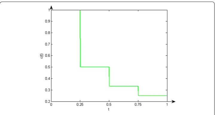
Remark . To make it clear for the reader whatc(t) is, we give a special example ofc(t), e.g., lettingk= ,t=,t=,t=,c= –,c= –,c= –, we can get the graph of c(t). For details, see Figure .
Such problems were first studied by Zhang and Feng []. By using the transformation technique to deal with impulsive term of second impulsive differential equations, the au-thors obtained the existence results of positive solutions by using fixed point theorems in a cone. But they only gave the sufficient conditions for the existence of finite positive solutions. In fact, there is almost no paper that considers the existence of infinitely many
positive solutions for second order singular impulsive parametric equations; for details, see [–].
For the caseλ= , a= ,b= ,h(t)≡ ont∈Jandck= (k= , , . . . ,n), problem
(.) reduces to the problem studied by Kaufmann and Kosmatov in []. By using Kras-nosel’ski˘ı’s fixed point theorem and Hölder’s inequality, the authors showed the existence of countably many positive solutions. The other related results can be found in [–]. However, there are almost no papers considering a second order impulsive parametric equation with infinitely many singularities. To identify a few, we refer the reader to [–] and the references therein.
The main reasons are thatλ= andck= (k= , , . . . ,n) in problem (.). Ifλ= , then
it is very difficult to be concerned with determining values ofλ, for which there exist
in-finitely many positive solutions. On the other hand, ifck= (k= , , . . . ,n), then there
exist singular points and impulsive points in the same problem, which leads to many dif-ficulties in defining the interval [τi, –τi], whereti+≤τi≤ti. The goal of this paper is to
seek new methods to solve these difficulties and to give some new sufficient conditions to guarantee that problem (.) has two infinite families of positive solutions.
2 Preliminaries
In this section, we collect some definitions and lemmas for the convenience of later use and reference.
Definition . A functionx(t) is said to be a solution of problem (.) onJif: (i) x(t)is absolutely continuous on each interval(,t]and(tk,tk+],k= , , . . . ,n; (ii) for anyk= , , . . . ,n,x(tk+),x(t–k)exist andx(tk–) =x(tk);
(iii) x(t)satisfies (.).
We shall reduce problem (.) to a system without impulse. To this goal, firstly by means of the transformation
x(t) =c(t)y(t), (.)
we convert problem (.) into
⎧ ⎪ ⎪ ⎨ ⎪ ⎪ ⎩
–λy(t) =c–(t)ω(t)f(t,c(t)y(t)), t∈J, ay() –by() =h(s)c(s)y(s)ds,
ac()y() +bc()y() =h(s)c(s)y(s)ds.
(.)
It follows from (.), (.) and (.) that we can obtain the following lemma.
Lemma . Assume that(H)-(H)hold.Then
(i) ify(t)is a solution of problem(.)onJ,thenx(t) =c(t)y(t)is a solution of problem (.)onJ;
Lemma . If(H)-(H)hold,then problem(.)has a solution y,and y can be expressed in the form
y(t) =λ–
H(t,s)c–(s)ω(s)fs,c(s)y(s) ds, (.)
where
H(t,s) =G(t,s) + A(t)
–μ
G(s,τ)c(τ)h(τ)dτ, (.)
G(t,s) =
d
⎧ ⎨ ⎩
(b+as)(b+a( –t)), ≤s≤t≤,
(b+at)(b+a( –s)), ≤t≤s≤, (.)
A(t) = (a+b–at)c() +a+b
dc() , d=a(a+ b).
Proof First suppose thatyis a solution of problem (.). It is easy to see by integration of problem (.) that
y(t) =y() –λ–
t
c–(s)ω(s)fs,c(s)y(s) ds, (.)
y(t) =y() +y()t–λ–
t
(t–s)c–(s)ω(s)fs,c(s)y(s) ds. (.)
Lettingt= in (.), (.), we find
y() =y() –λ–
c–(s)ω(s)fs,c(s)y(s) ds,
y() =y() +y() –λ–
( –s)c–(s)ω(s)fs,c(s)y(s) ds.
(.)
Combining the boundary conditionay() –by() =h(s)c(s)y(s)ds,ac()y() +bc()×
y() =h(s)c(s)y(s)dsand (.), we obtain
y() = aλ –
a+ b
( –s)c–(s)ω(s)fs,c(s)y(s) ds
+ bλ
–
a+ b
c–(s)ω(s)fs,c(s)y(s) ds
+ –c()
(a+ b)c()
h(s)c(s)y(s)ds, (.)
y() = bλ –
a+ b
( –s)c–(s)ω(s)fs,c(s)y(s) ds
+ b
λ–
a(a+ b)
c–(s)ω(s)fs,c(s)y(s) ds
+b+ (a+b)c()
a(a+ b)c()
Substituting (.), (.) into (.) and letting
The proof of the lemma is complete.
and
Di=
–μ+Ai
–θi
θi c(τ)h(τ)dτ
–μ , D=
–μ+AM
c(τ)h(τ)dτ
–μ ,
AM=max
t∈J A(t), Ai=
(a+b–aθi)c() +a+b
dc() .
Proof It is obvious that (.) and (.) hold by the definition ofG(t,s) andH(t,s). Next, we show that (.) holds fort∈[θi, –θi],s∈J. In fact, ifs≤t, it follows from
(.) that
G(t,s)≥
d(b+as)(b+aθi) =
b(b+aθi)
d .
Similarly, we can prove thatG(t,s)≥b(b+aθi)
d ,∀≤t≤s≤.
Therefore,
G(t,s)≥αi∗, ∀t∈[θi, –θi],s∈J.
And then, by (.), fort∈[θi, –θi],s∈J, we have
H(t,s) =G(t,s) + A(t)
–μ
G(s,τ)c(τ)g(τ)dτ
≥αi∗+ Ai
–μ
G(s,τ)c(τ)g(τ)dτ
≥αi∗+ Ai
–μ
–θi
θi
G(s,τ)c(τ)g(τ)dτ
≥αi∗+Aiα
∗ i
–μ
–θi
θi
c(τ)g(τ)dτ
=αi∗Di.
So,
H(t,s)≥αi, ∀t∈[θi, –θi],s∈J.
The proof is complete.
Lemma .(see []) Let E be a real Banach space and K be a cone in E.For r> ,define Kr={x∈K:x<r}.Assume that T:K¯r→K is completely continuous such that Tx=x
for x∈∂Kr={x∈K:x=r}.
(i) IfTx ≥ xforx∈∂Kr,theni(T,Kr,K) = .
(ii) IfTx ≤ xforx∈∂Kr,theni(T,Kr,K) = .
Lemma .(Hölder) Let e∈Lp[a,b]with p> ,h∈Lq[a,b]with q> ,and
p+
q= .Then
eh∈L[a,b]and
Let e∈L[a,b],h∈L∞[a,b].Then eh∈L[a,b]and
eh≤ eh∞.
3 The existence of two infinite families of positive solutions
In this part, applying the well-known fixed point index theory in a cone, we get the
op-timal interval of parameterλin which problem (.) has two infinite families of positive
solutions. We remark that our methods are entirely different from those used in [–].
LetE=C[, ]. ThenEis a real Banach space with the norm · defined by
y=max
t∈J y(t), y∈E.
Define a coneKinEby
K=
y∈E:y(t)≥,t∈J, min
t∈[θ,–θ]y(t)≥δDy,t∈J
, (.)
whereδD=Dδ.
Remark . It follows from the definition ofδandDthat <δD< .
DefineTλ:K→Kby
(Tλy)(t) =
λ
H(t,s)ω(s)c–(s)fs,c(s)y(s) ds. (.)
Theorem . Assume that(H)-(H)hold.Then Tλ(K)⊂K and Tλ:K→K is completely continuous.
Proof Fory∈K, it follows from (.) and (.) that
(Tλy)(t) =
λ
H(t,s)ω(s)c–(s)fs,c(s)y(s) ds
≤
λD
G(s,s)ω(s)c–(s)fs,c(s)y(s) ds, t∈J. (.)
It follows from (.), (.) and (.) that
min
t∈[θ,–θ](Tλy)(t) =
λt∈min[θ,–θ]
H(t,s)ω(s)c–(s)fs,c(s)y(s) ds
≥
λδ
G(s,s)ω(s)c–(s)fs,c(s)y(s) ds ≥
λ δ
DD
G(s,s)ω(s)c–(s)fs,c(s)y(s) ds ≥δDTλy.
Next, by similar arguments of Theorem in [] one can prove thatTλ:K→Kis
Remark . From (.), we know thaty∈Eis a solution of problem (.) if and only ify
is a fixed point of operatorTλ.
Let{θi}∞i= be such thatti+<θi<ti,i= , , . . . . Then, for anyi∈N, we define the cone
Kθiby
Kθi=y∈E:y(t)≥,t∈J, min t∈[θi,–θi]
y(t)≥δiDy,t∈J
, (.)
where
δiD= δi
D, δi= b+aθi
a+b , i= , , . . . . (.)
Remark . Assume that (H)-(H) hold. ThenTλ(Kθi)⊂KθiandTλ:Kθi→Kθiis
com-pletely continuous.
Next, using Lemmas .-., we give our main results under the caseω∈LP[, ];p> ,
p= andp=∞.
For convenience, we write
fδρDρ=min
min t∈[θ,–θ]
f(t,y)
ρ :y∈[δDρ,ρ]
, fρ=max
max t∈J
f(t,y)
ρ :y∈[,ρ]
,
Kρθi={y∈Kθi:y<ρ}, ρ> .
Firstly, we consider the casep> .
Theorem . Assume that(H)-(H)hold.Let{ri}∞i=,{γi}∞i=and{Ri}∞i=be such that
Ri+<δiDri<ri<cmδiDγi<cMγi<Ri, i= , , . . . .
For each natural number i,let f satisfy the following conditions:
(H) fcMri≤landf
cMRi
≤l,where
<l≤max
λcm
cMGqωp
, λcm
cMGω∞,
λcm
cMβω
; (.)
(H) fcmcMδγiDiγi≥η,whereη> .
Then there existsτ> such that,for <λ<τ,problem(.)has two infinite families of positive solutions x()iλ(t),x()iλ(t)andmaxt∈Jx()iλ(t) >cmδiDγi,i= , , . . . .
Proof Letτ =inf{τi},τi=αic–mξ η( – θi)γi–,i= , , . . . . Then, for <λ<τ, (.) and
Theorem . imply thatTλ:K→Kis completely continuous.
Lett∈J,y∈∂Kriθi. Then ≤c(t)y(t)≤cMri. Therefore, fort∈J,y∈∂Kriθi, it follows
fromfcMri≤lthat
(Tλy)(t) =
λ
H(t,s)ω(s)c–(s)fs,c(s)y(s) ds ≤
λc
–
m
≤
λc
–
mHqωplcMri
≤
ri<ri. (.)
Consequently, fory∈∂Kriθi, we haveTλy<y, i.e., by Lemma .,
i(Tλ,Kriθi,Kθi) = . (.)
Similarly, fory∈∂KRiθi, we haveTλy<y, and then it follows from Lemma . that
i(Tλ,KRiθi,Kθi) = . (.)
On the other hand, let
y∈ ¯Kγi
δiDγiθi=
y∈Kθi:y ≤γi,t∈min
[θi,–θi]
y(t)≥δiDγi
,
then ≤c(t)y(t)≤cMy ≤cMγi. And hence, it follows from (.) and (.) that
Tλy ≤
λc
–
mHqωplcMγi<γi. (.)
Furthermore, for y∈ ¯Kγi
δiDγiθi, we have c(t)y(t) ≤cMγi, t∈ J, mint∈[θiD,–θi]c(t)y(t)≥
cmδiDγi, and then
min t∈[θi,–θi]
(Tλy)(t) = min t∈[θi,–θi]
λ
H(t,s)ω(s)c–(s)fs,c(s)y(s) ds
≥
λαic
–
mξ
fs,c(s)y(s) ds
≥
λαic
–
mξ
–θi
θi
fs,c(s)y(s) ds ≥
λαic
–
mξ( – θi)η
>
ταic
–
mξ( – θi)η
=γi. (.)
Lety≡ δiDγi+γi andF(t,y) = ( –t)Tλy+ty, thenF:J× ¯KδγiDiγiθi→Kθi is completely
continuous. From the analysis above, we obtain for (t,y)∈J× ¯Kγi
δiDγiθi,
F(t,y)∈Kγi
δiDγiθi. (.)
Therefore, fort∈J,y∈∂Kγi
δiDγiθi, we haveF(t,y)=y. Hence, by the normality property
and the homotopy invariance property of the fixed point index, we obtain
iTλ,Kγi
δiDγiθi,Kθi =i
Consequently, by the solution property of the fixed point index,Tλhas a fixed pointy()iλ
andy()iλ ∈K γi
δiDγiθi. By Lemma . and Remark ., it follows thaty
()
iλ is a solution to problem
(.), and
max t∈J y
()
iλ(t)≥t∈min [θi,–θi]
y()iλ(t) >δiDγi.
Therefore, it follows from Lemma . that problem (.) has a solutionx()iλ(t) =c(t)y()iλ(t) with
max t∈J x
()
iλ(t) =maxt∈J c(t)y ()
iλ(t)≥t∈min [θi,–θi]
c(t)y()iλ(t) >cmδiDγi.
On the other hand, from (.), (.) and (.) together with the additivity of the fixed point index, we get
iTλ,KRiθi\
¯
Kriθi∪ ¯K
γi
δiDγiθi ,Kθi
=i(Tλ,KRiθi,Kθi) –i
Tλ,Kγi
δiDγiθi,Kθi –i(Tλ,Kriθi,Kθi)
= – – = –. (.)
Hence, by the solution property of the fixed point index,Tλhas a fixed pointy()iλ and
y()iλ ∈KRi\(K¯ri∪ ¯KδγiDiγiθi). By Lemma . and Remark ., it follows thaty
()
iλ is also a solution
to problem (.), andy()iλ =y ()
iλ. And then, by Lemma ., we have problem (.) has another
solutionx()iλ(t) =c(t)y ()
iλ(t). Sincei∈N was arbitrary, the proof is complete.
The following results deal with the casep=∞.
Theorem . Assume that(H)-(H)hold.Let{ri}∞i=,{γi}∞i=and{Ri}∞i=be such that
Ri+<δiDri<ri<cmδiDγi<cMγi<Ri, i= , , . . . .
For each natural number i,letf satisfy(H)and(H),then there existsτ > such that, for <λ<τ,problem(.)has two infinite families of positive solutions x()iλ(t),x
()
iλ(t)and
maxt∈Jx()iλ(t) >cmδiDγi,i= , , . . . .
Proof LetGω∞replaceGqωpand repeat the previous argument.
Finally, we consider the case ofp= .
Theorem . Assume that(H)-(H)hold.Let{ri}∞i=,{γi}∞i=and{Ri}∞i=be such that
Ri+<δiDri<ri<cmδiDγi<cMγi<Ri, i= , , . . . .
For each natural number i,let f satisfy(H)and(H),then there existsτ> such that, for <λ<τ,problem(.)has two infinite families of positive solutions x()iλ(t),x
()
iλ(t)and
maxt∈Jx()iλ(t) >cmδiDγi,i= , , . . . .
Remark . Comparing with Kaufmann and Kosmatov [], the main features of this paper are as follows.
(i) The solvable intervals of positive parameterλare available. (ii) Two infinite families of positive solutions are obtained. (iii) ck> –,k= , , . . . ,n, not onlyck≡.
4 Examples
From Section , it is not difficult to see that (H) and (H) play an important role in the
proof that problem (.) has two infinite families of positive solutions. So, we firstly provide an example of families of functionsω(t) satisfying conditions (H) and (H). And then we consider a boundary value problem associated with problem (.).
+
Example . Letω(t) be defined as in Example .. Consider the following boundary value problem:
Similarly, a simple calculation shows thatA(t) =
G(t,s) =
Now we consider the multiplicity of positive solutions for problem (.). Letf(t,x) =
ωβ(t+ )x. It follows from the definitions ofω(t),f(t,x),c(t) andh(t) that
conditions (H)-(H) hold. Hence, we only verify the other conditions of our main results.
Letθi=–(i+) . Thenθi∈(,). ForRi=i,γi=×i andri=×i,i= , , . . . ,
By a direct calculation, we have
f(t,x) =
Hence, by Theorem ., problem (.) has two infinite families of positive solutions
x()iλ(t) andx()iλ(t) for <λ<τ=inf{αiξ η( – θi)γi–},i= , , . . . .
Acknowledgements
This work is sponsored by the National Natural Science Foundation of China (11301178)and the Beijing Natural Science Foundation (1163007), the Scientific Research Project of Construction for Scientific and Technological Innovation Service Capacity (71E1610973) and the teaching reform project of Beijing Information Science & Technology University (2015JGYB41). The authors are grateful to anonymous referees for their constructive comments and suggestions which have greatly improved this paper.
Competing interests
The authors declare that they have no competing interests.
Authors’ contributions
Publisher’s Note
Springer Nature remains neutral with regard to jurisdictional claims in published maps and institutional affiliations.
Received: 16 December 2016 Accepted: 17 May 2017 References
1. Zhang, X, Feng, M: Transformation techniques and fixed point theories to establish the positive solutions of second-order impulsive differential equations. J. Comput. Appl. Math.271, 117-129 (2014)
2. Liu, L, Hu, L, Wu, Y: Positive solutions of two-point boundary value problems for systems of nonlinear second order singular and impulsive differential equations. Nonlinear Anal.69, 3774-3789 (2008)
3. Agarwal, RP, Franco, D, O’Regan, D: Singular boundary value problems for first and second order impulsive differential equations. Aequ. Math.69, 83-96 (2005)
4. Lin, X, Jiang, D: Multiple solutions of Dirichlet boundary value problems for second order impulsive differential equations. J. Math. Anal. Appl.321, 501-514 (2006)
5. Liu, Y, O’Regan, D: Multiplicity results using bifurcation techniques for a class of boundary value problems of impulsive differential equations. Commun. Nonlinear Sci. Numer. Simul.16, 1769-1775 (2011)
6. Xu, J, Wei, Z, Ding, Y: Existence of positive solutions for a second order periodic boundary value problem with impulsive effects. Topol. Methods Nonlinear Anal.43, 11-21 (2014)
7. Hao, X, Liu, L, Wu, Y: Positive solutions for second order impulsive differential equations with integral boundary conditions. Commun. Nonlinear Sci. Numer. Simul.16, 101-111 (2011)
8. Kaufmann, ER, Kosmatov, N: A multiplicity result for a boundary value problem with infinitely many singularities. J. Math. Anal. Appl.269, 444-453 (2002)
9. Liang, SH, Zhang, JH: The existence of countably many positive solutions for nonlinear singularm-point boundary value problems. J. Comput. Appl. Math.214, 78-89 (2008)
10. Ji, D, Bai, Z, Ge, W: The existence of countably many positive solutions for singular multipoint boundary value problems. Nonlinear Anal.72, 955-964 (2010)
11. Kosmatov, N: Countably many solutions of a fourth order boundary value problem. Electron. J. Qual. Theory Differ. Equ.2004, 12 (2004)
12. Bonanno, G, Bella, BD, Henderson, J: Infinitely many solutions for a boundary value problem with impulsive effects. Bound. Value Probl.2013, 278 (2013)
13. Graef, JR, Heidarkhani, S, Kong, L: Infinitely many solutions for systems of multi-point boundary value problems using variational methods. Topol. Methods Nonlinear Anal.42, 105-118 (2013)
14. Afrouzi, GA, Hadjian, A, Shokooh, S: Infinitely many solutions for a Dirichlet boundary value problem with impulsive condition. UPB Sci. Bull., Ser. A77, 1-22 (2015)
15. Guo, D, Lakshmikantham, V: Nonlinear Problems in Abstract Cones. Academic Press, New York (1988) 16. Zhao, A, Yan, W, Yan, J: Existence of positive periodic solution for an impulsive delay differential equation. In: