R E S E A R C H
Open Access
MMSE-based joint source and relay
optimization for interference MIMO relay
systems
Khoa Xuan Nguyen
*, Yue Rong and Sven Nordholm
Abstract
In this paper, we investigate the transceiver design for amplify-and-forward (AF) interference multiple-input multiple-output (MIMO) relay communication systems when the direct links between the source and destination nodes are taken into consideration. The minimum mean-squared error (MMSE) of the signal waveform estimation at the destination nodes is chosen as the design criterion to optimize the source, relay, and receiver matrices for interference suppression. As the joint source, relay, and receiver optimization problem is nonconvex with matrix variables, a globally optimal solution is computationally intractable to obtain. We propose two iterative algorithms to provide computationally efficient solutions to the original problem through solving convex subproblems. These two algorithms provide efficient performance-complexity trade-off. Simulation results demonstrate that the proposed algorithms converge quickly after a few iterations and significantly outperform existing scheme in terms of the system bit error rate.
Keywords: Interference channel; MIMO relay; Direct link; MSE
1 Introduction
Relay-aided multiple-input multiple-output (MIMO) communication technology has attracted great research interest recently [1,2]. By incorporating relay nodes in a MIMO system, the network coverage and reliability can be significantly improved. In a MIMO relay system, com-munication between source nodes and destination nodes can be assisted by single or multiple relays equipped with multiple antennas. The relays can either decode-and-forward (DF) or amplify-and-decode-and-forward (AF) the relayed signals [3]. In the AF scheme, the received signals are simply amplified (including a possible linear transforma-tion) through the relay precoding matrices before being forwarded to the destination nodes. Therefore, in gen-eral, the AF strategy has lower complexity and shorter processing delay than the DF strategy.
For single-user two-hop MIMO communication sys-tems with a single relay node, the optimal source and relay precoding matrices have been developed in [4]. For
*Correspondence: [email protected]
Department of Electrical and Computer Engineering, Curtin University of Technology, Kent Street, Bentley, WA 6102, Australia
a single-user two-hop MIMO relay system with multiple parallel relay nodes, the design of relay precoding matrices has been studied in [5]. Recent progress on the optimiza-tion of AF MIMO relay systems has been summarized in the tutorial of [2].
For MIMO interference channel, the idea of interference alignment (IA) [6] was developed for interference sup-pression by arranging the desired signal and interference into appropriated signal spaces. The idea of IA has been applied in interference MIMO relay systems in [7,8]. How-ever, there is still no general solution for IA as a number of conditions must be met. One main reason is that the number of dimensions required for IA is very large and it depends on the number of independent fading channels. This leads to high computational complexity and infeasi-bility in practical systems. In [9], an iterative algorithm has been proposed to optimize the source beamforming vec-tor and the relay precoding matrices to minimize the total source and relay transmit power such that a minimum signal-to-interference-plus-noise ratio (SINR) threshold is maintained at each receiver. Three iterative transceiver design algorithms to minimize either the matrix-weighted sum mean-squared error (SMSE) or the total leakage have
been developed in [10]. However, the works in [7,10] did not take the direct source-destination links into consider-ation.
The direct links between the source and destination nodes provide valuable spatial diversity to the MIMO relay system and should not be ignored. In this paper, we investigate the transceiver design for AF interfer-ence MIMO relay communication systems where multiple source nodes transmit information simultaneously to the destination nodes with the aid of multiple relay nodes, and each node is equipped with multiple antennas. The direct source-destination links are taken into account for the design of the transceivers. We aim at optimizing the source, relay, and receiver matrices to suppress the inter-ference and minimize the SMSE of the signal waveform estimation at the destination nodes, subjecting to trans-mission power constraints at the source and relay nodes. The SMSE criterion is chosen as it provides a good trade-off between performance and complexity. Since the joint source, relay, and receiver optimization problem is non-convex with matrix variables, a globally optimal solution is computationally intractable to obtain. We propose two iterative algorithms to provide computationally efficient solutions to the original problem through solving convex subproblems. In each iteration of the first algorithm, we first optimize all receiver matrices based on the source and relay matrices from the previous iteration. Then, we optimize all relay matrices using the receiver matrices in this iteration and the source matrices from the previous iteration. Finally, the source matrices are updated.
In the second algorithm, the receiver matrices are opti-mized in the same way as the first algorithm. How-ever, in contrast to the first algorithm, each source and relay matrix is optimized individually by fixing all other matrices. We show that both proposed algorithms con-verge. Comparing the two proposed algorithms, the first algorithm has a better MSE and bit error rate (BER) performance, while the second algorithm has a smaller per-iteration computational complexity. Such performance-complexity trade-off is very useful for practical MIMO relay communication systems. Simulation results demon-strate that the proposed algorithms outperform the exist-ing technique in terms of the system MSE and BER.
We assume that similar to [10], the two proposed algo-rithms are carried out at a central controlling unit, which can be any node in the system. The controlling unit has knowledge of the global channel state information (CSI). After the convergence of the algorithms, the controlling unit sends the information on the optimal source, relay, and receiver matrices to corresponding nodes.
The rest of this paper is organized as follows. The sys-tem model and problem formulation are introduced in Section 2. Two iterative joint source, relay, and receiver matrices design algorithms are developed in Section 3.
Simulation results are presented in Section 4 to demon-strate the performance of the proposed algorithms. Con-clusions are drawn in Section 5.
Throughout this paper, scalars are denoted with lower-or uppercase nlower-ormal letters, and vectlower-ors and matrices are denoted with bold-faced lower- and uppercase let-ters, respectively. Superscripts(·)T,(·)H, and(·)−1denote the matrix transpose, conjugate transpose, and inverse, respectively; tr() stands for the trace of a matrix; vec() stacks columns of a matrix on top of each other into a single vector; bd() denotes a block-diagonal matrix; ⊗ represents the Kronecker product,E[ ] denotes the sta-tistical expectation; and In stands for then×nidentity matrix.
2 System model and problem formulation
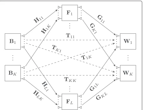
We consider a two-hop interference MIMO relay
commu-nication system where K source-destination pairs
com-municate simultaneously with the aid of a network of
L-distributed relay nodes as shown in Figure 1. The kth source node and thekth destination node are equipped with Nsk and Ndk antennas, respectively, k = 1,· · ·,K, and the number of antennas at thelth relay node isNrl, l=1,· · ·,L.
Using half duplex relay nodes, the communication between source and destination pairs is completed in two time slots. At the first time slot, the kth source node transmits anNsk×1 signal vector
xsk =Bksk, k=1,· · ·,K (1)
to the relay nodes and the destination nodes, whereskis the d×1 information-carrying symbol vector andBk is theNsk×dsource precoding matrix. The received signal vectors at thelth relay node and thekth destination node are given by
yrl =
whereHlk is theNrl×Nsk MIMO fading channel matrix between thekth source node and thelth relay node,Tkmis theNdk×NsmMIMO fading channel matrix between the mth source node and thekth destination node,vrl is the Nrl×1 additive white Gaussian noise (AWGN) vector at thelth relay node with zero mean and covariance matrix
EvrlvHrl
= σ2
rlINrl,l = 1,· · ·,L, andvd1k is theNdk×1 AWGN vector at thekth destination node at the first time slot with zero mean and covariance matrixEvd1kvHd1k
=
σ2
dkINdk,k=1,· · ·,K.
During the second time slot, the received signal vec-tor at thelth relay node is amplified with theNrl ×Nrl precoding matrixFlas
xrl=Flyrl, l=1,· · ·,L. (4)
The precoded signal vectorxrl is forwarded to the des-tination nodes. The received signal vector at the kth destination node is given by
yd2k = L
l=1
Gklxrl+vd2k, k=1,· · ·,K (5)
whereGklis theNdk×NrlMIMO channel matrix between thelth relay node and thekth destination node andvd2k is theNdk×1 AWGN vector at thekth destination node at the second time slot with zero mean and covariance matrixEvd2kvHd2k
=σ2
dkINdk,k=1,· · ·,K.
From Equations 1 to 5, the signal vector received at the
kth destination node over two consecutive time slots is
yk = at thekth destination node at the second time slot.
Due to their simplicity, linear receivers are used at the destination nodes to retrieve the transmitted signals. Thus, the estimated signal vector at the kth destination node can be written as
ˆ ces for the direct link and the relay link, respectively. In Equations 6 and 7, we have
ˆ
In Equations 1 and 4, the transmission power con-straints at the source and relay nodes can be written as
where Psk and Prl denote the power budget at the kth source node and the lth relay node, respectively, and
EyrlyHrl = Km=1HlmBmBHmHHlm +σrl2INrl is the covari-ance matrix of the received signal vector at thelth relay node.
In this paper, we aim at optimizing the source precoding matrices {Bk} = {Bk,k = 1,· · ·,K}, the relay precod-ing matrices{Fl} = {Fl,l = 1,· · ·,L}, and the receiver weight matrices{Wk} = {Wk, k=1,· · ·,K}, to minimize the sum-MSE of the signal waveform estimation at the destination nodes under transmission power constraints at the source and relay nodes. We would like to mention that minimal MSE (MMSE) is a sensible design criterion based on the links of MSE to other performance measures in MIMO systems such as mutual information and SINR [4,11].
From Equation 8, the MSE of thekth source-destination pair can be calculated as
MSEk = tr
whereH˜kmis the equivalent MIMO channel matrix from the mth source node to thekth destination node,Ck = Ev¯Tdk, vTd1kTv¯Hdk, vHd1k and k are the covariance matrices of the equivalent noise and the interference at the
˜ matrix between the mth source node and the lth relay node.
From Equations 9 to 11, the optimal source, relay, and receiver matrix design problem can be written as
min
3 Proposed source, relay, and receiver matrix design algorithms
The problem (Equations 12 to 14) is highly nonconvex with matrix variables, and a globally optimal solution is intractable to obtain. In this section, we propose two iter-ative algorithms to solve the problem (Equations 12 to 14) by optimizing{Wk},{Bk}, and{Fl}in an alternating way through solving convex subproblems.
3.1 Proposed Algorithm 1
In each iteration of this algorithm, we first optimize{Wk} based on{Bk}and{Fl}from the previous iteration. Then, we optimize all relay matrices based on {Wk} from the current iteration and {Bk} from the previous iteration. Finally, we optimize all source matrices using{Wk}and {Fl}from the current iteration.
It can be seen from Equation 11 thatWk only affects MSEk. Thus, with given{Fl}and{Bk}, the optimal linear receiver matrix which minimizes MSEk in Equation 11 is the solution to the following unconstrained optimization problem
min Wk
MSEk. (15)
The solution to the problem (Equation 15) is the well-known MMSE receiver [12] given by
Wk = receiver matrices {Wk} and source precoding matrices {Bk}, the sum-MSE SMSE= Kk=1MSEkcan be rewritten
is independent offand fork,m=1,· · ·,K,l=1,· · ·,L matrix between the lth relay node and the kth desti-nation node and T¯km = WHk1TkmBm is the equivalent direct link MIMO channel matrix between themth source node and thekth destination node. The detailed proof of Equation 17 is given in Appendix 6.1.
By introducing the relay transmit power constraints in Equation 10 can be rewritten as
fHD¯lf≤Prl, l=1,· · ·,L. (23)
In Equations 17 and 23, the relay matrix optimization problem can be written as
min
f ψ1(f) (24)
s.t. fHD¯lf≤Prl, l=1,· · ·,L. (25)
The optimization problem (Equations 24 to 25) is a quadratically constrained quadratic programming (QCQP) problem [13]. From Equation 21, we can see that Qkl, k = 1,· · ·,K, l = 1,· · ·,L are positive semidefi-nite (PSD) matrices, and thus from Equation 19,Qk,k =
1,· · ·,Kare PSD matrices. Moreover, it can be seen from Equation 22 thatDll,l = 1,· · ·,Lare PSD matrices, and thus, D¯l, l = 1,· · ·,Lare PSD matrices. Therefore, the QCQP problem (Equations 24 to 25) is convex and can be efficiently solved by the interior-point method [13]. In particular, the problem (Equations 24 to 25) can be solved by the CVX MATLAB toolbox for disciplined convex programming [14].
Let us introduce bk = vec(Bk), k = 1,· · ·,K. With given receiver matrices {Wk} and relay matrices {Fl},
the sum-MSE can be rewritten as a function of b =
1(b)= optimization process as it is independent ofband
U = bd(U1,U2,· · ·,UK) (27)
proof of Equation 26 is given in Appendix 7.1.
Let us introduce Eij = Id ⊗ obtained by solving the following problem
min are PSD matrices, and thus from Equation 27,Uis PSD. Moreover, it can be seen that E¯m, m = 1,· · ·,K and El,l = 1,· · ·,Lare PSD matrices. Therefore, the prob-lem (Equations 31 to 33) is a convex QCQP probprob-lem and can be solved by the CVX MATLAB toolbox [14] for disciplined convex programming.
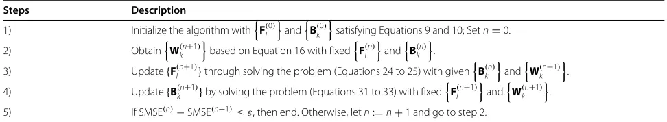
The steps of applying the proposed Algorithm 1 to opti-mize {Bk}, {Fl}, and {Wk} are summarized in Table 1, where the superscript (n) denotes the variable at the
nth iteration, and ε is a small positive number up to which convergence is acceptable. Since all subproblems (Equation 15, 24 to 25, and 31 to 33) are convex, the solu-tion to each subproblem is optimal. Thus, the value of the objective function (Equation 12) monotonically decreases after each iteration. Moreover, the value of Equation 12 is
lower bounded by at least zero. Therefore, the proposed Algorithm 1 is guaranteed to converge.
3.2 Proposed Algorithm 2
In the proposed Algorithm 1, all source precoding matri-ces are optimized together through b, while all relay precoding matrices are updated together throughf. Since the dimensions ofb and fare Kk=1Nskd and Ll=1Nrl2, respectively, the computational complexity of solving the QCQP problems (Equations 24 to 25 and 31 to 33) using
the interior point method [15] isO Kk=1Nskd
, respectively. Therefore, the
computa-tional complexity at each iteration of the proposed
Algo-rithm 1 isO Kk=1Nskd
be very high for interference MIMO relay systems with a largeK andL. To reduce the per-iteration complexity, in this subsection, we develop an iterative algorithm where each source and relay matrix is optimized individually by fixing all other matrices.
Adopting notations from proposed Algorithm 1, with given receiver matrices{Wk}, source precoding matrices {Bk}, and relay precoding matricesFj,j= 1,· · ·,L,j=l, the sum-MSE can be rewritten as a function ofFlas
SMSE =
Table 1 Procedure of solving the problem (Equations 12 to 14) by the proposed Algorithm 1
Using the identities in Equations 43 to 45, the SMSE in Equation 34 can be written as
ψ2(fl)= K
k=1
⎡
⎣(Ok,l,kfl−akl)H(Ok,l,kfl−akl)+fHl Qklfl+rkl
+ K
m=1,m=k
Ok,l,mfl−dk,l,m H
Ok,l,mfl−dk,l,m ⎤⎦
(36)
where fork,m=1,· · ·,K,l=1,· · ·,L
akl = vec(Akl)
rkl = tr ⎛ ⎝ L
j=1,j=l
σ2
rjG¯kjFjFHj G¯Hkj+σdk2WHkWk ⎞ ⎠
dk,l,m = vec
Dk,l,m
.
Note that since the terms rkl in Equation 36 are inde-pendent of fl, they can be ignored when optimizing fl. The relay transmit power constraint in Equation 10 can be rewritten as
fHl Dllfl≤Prl. (37)
Based on Equations 36 and 37, the optimal fl can be obtained by solving the following problem for each l =
1,· · ·,L
min fl
ψ2(fl) s.t. fHl Dlfl≤Prl. (38)
The problem (Equation 38) is a QCQP problem and can be solved effectively using the CVX toolbox.
With given receiver matrices {Wk}, relay precoding matrices {Fl}, and source precoding matrices Bj, j = 1,· · ·,K,j=k, the SMSE can be rewritten as a function ofbkas
2(bk) = (Skkbk−vec(Id))H(Skkbk−vec(Id)) +bHkUkbk+zk
where
zk = K
m=1,m=k
(Smmbm−vec(Id))H(Smmbm−vec(Id))
+bHmUmbm
+t2, k=1,· · ·,K.
By introducingclk = σrl2tr
FlFHl
+ K
j=1,j=kbHj Eljbj, k=1,· · ·,K,l=1,· · ·,L, the optimalbkcan be obtained by solving the following problem for eachk=1,· · ·,K
min bk
2(bk) (39)
s.t. bHkbk ≤Psk (40)
bHkElkbk ≤Prl−clk, l=1,· · ·,L. (41)
The problem (Equations 39 to 41) is a QCQP prob-lem and can be solved by the CVX MATLAB toolbox [14] for disciplined convex programming. The steps of using the proposed Algorithm 2 to optimize{Bk},{Fl}, and {Wk} are summarized in Table 2. Similar to the analysis used to the proposed Algorithm 1, since all subproblems (Equations 15, 38, and 39 to 41) are convex, the solu-tion to each subproblem is optimal. Thus, the value of the objective function (Equation 12) monotonically decreases after each iteration. Moreover, the value of Equation 12 is lower bounded by at least zero. Therefore, the conver-gence of the proposed Algorithm 2 follows directly from this observation.
Since the dimensions of bk and fl are Nskd and Nrl2, respectively, the computational complexity of solving the QCQP problems (Equations 38 and 39 to 41) is
O(Nskd)3
and ONrl6, respectively. Thus, the com-putational complexity at each iteration of the proposed Algorithm 2 is O Kk=1(Nskd)3+ Ll=1Nrl6
, which is lower than the per-iteration computational complexity of the proposed Algorithm 1. However, we will see through numerical simulations that the proposed Algorithm 1 has a better MSE and BER performance than that of the pro-posed Algorithm 2. Such performance-complexity trade-off is very useful for practical interference MIMO relay communication systems.
4 Numerical examples
In this section, we illustrate the performance of the proposed algorithms through numerical simulations. All channel matrices have independent and identically dis-tributed (i.i.d.) complex Gaussian entries with zero mean and unit variance. The noises are i.i.d. Gaussian with zero mean and unit variance. Unless explicitly mentioned, the
Table 2 Procedure of solving the problem (Equations 12 to 14) by the proposed Algorithm 2
Steps Description
1) Initialize the algorithm withF(l0)andB(k0)satisfying Equations 9 and 10; Setn=0. 2) ObtainW(kn+1)based on Equation 16 with fixedFl(n)andB(kn).
3) Forl=1,· · ·,L, updateFl(n+1)through solving the problem (Equation 38) with givenB(kn),W(kn+1), andF(jn),j=1,· · ·,L,j=l. 4) Fork=1,· · ·,K, updateBk(n+1)by solving the problem (Equations 39 to 41) with fixedF(ln+1),W(kn+1), andBj(n),j=1,· · ·,K,
j=k.
QPSK constellations are used to modulate the source sym-bols. For the sake of simplicity, we setd= 2 and assume that all nodes have three antennas, i.e.,Nsk=Ndk =Nrl=
3,k = 1,· · ·,K,l = 1,· · ·,L, all source nodes have the same power budget asPsk = 15dB,k = 1,· · ·,K, and all relay nodes have the same power budget asPrl = P, l=1,· · ·,L.
For all simulation examples, the simulation results
are averaged over 105 independent channel
realiza-tions. Unless explicitly mentioned, we assume that there
are K = 4 source-destination pairs and L = 5
relay nodes in the interference MIMO relay system. The proposed algorithms are initialized at! F(l0) =
Prl/tr Kk=1H¯lkH¯Hlk+INrl
INrl, l = 1,· · ·,L, and
B(k0) = √Psk/NskINsk, k = 1,· · ·,K. We would like to mention that when the matrix weight is identity matrix, the performance of the matrix-weighted sum-MSE min-imization (WMSE) algorithm without power control in [10] is similar to the proposed Algorithm 2 without con-sidering the direct links.
In the first example, we study the performance of the proposed algorithms at different number of iterations. We also compare the performance of the algorithms when the direct links are ignored. Moreover, the performance of the total leakage minimization (TLM) algorithm in [10] is included as a benchmark. Figure 2 shows the MSE per-formance of the proposed algorithms versusPat different number of iterations for the first source-destination pair
(k = 1). It can be seen from Figure 2 that both
pro-posed algorithms perform better than the TLM algorithm when the direct links are ignored. The performance of both proposed algorithm is significantly improved when the direct links are taken into account. For both proposed
Figure 2Example 1: MSE versusPat different number of iterations.
algorithms, the MSE reduces with increasing number of iterations. Moreover, it can be observed that after ten iterations, the decreasing of the MSE is small. Thus, we suggest that only ten iterations need to be carried out in practice to achieve a good performance-complexity trade-off. It can also be seen from Figure 2 that both proposed algorithms have almost the same MSE performance at convergence.
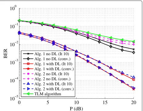
For this example, the average BER of all source-destination pairs yielded by both proposed algorithms versus P at different number of iterations is shown in Figure 3. It can be clearly seen that the proposed algo-rithms with direct links yield much smaller BER than the case when the direct links are ignored, especially at highPlevel. We can also observe from Figure 3 that the proposed Algorithm 1 has a slightly better BER perfor-mance than the proposed Algorithm 2. It can also be seen from Figure 3 that when the direct links are ignored, the proposed algorithms perform better than the TLM algorithm.
In the second example, we study the performance of the proposed algorithms with different number of relay nodes. Figure 4 shows the MSE performance of the
proposed Algorithm 1 versusP with L= 5 andL=10.
It can be seen that by doubling the number of relay nodes, a power gain of 10 dB is obtained at the MSE of 0.2.
For this example, the BER performance of the proposed
Algorithm 1 with L = 5 and L = 10 is illustrated in
Figure 5. It can be seen that by increasing the number of relay nodes, the system spatial diversity is increased, and thus, a better BER performance is achieved. In particular, we observe that an 8 dB gain is obtained at the BER of 10−3 by increasingLfrom 5 to 10.
Figure 4Example 2: MSE versusPfor differentL.
In the next example, we study the performance of the proposed algorithms with different number of source-destination pairs. Figure 6 shows the BER performance of both proposed algorithms versusP. Moreover, the BER of both algorithms using the 16QAM modulation scheme is also illustrated in Figure 6. As expected, the system BER is increased when higher order constellations are used. We can also obverse from Figure 6 that with a smaller number of source-destination pairs, the number of inter-ference channels decreases which yields a better BER performance. Interestingly, the BER difference between
the two proposed algorithm becomes bigger whenK=3.
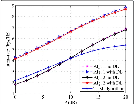
In the last example, we study the performance of the proposed algorithms on the achievable end-to-end sum-rates of all source-destination pairs. It can be seen from Figure 7 that, as expected, with the direct links taken into
Figure 5Example 2: BER versusPfor differentL.
Figure 6Example 3: BER versusPfor differentK.
account, both proposed algorithms achieve a higher sum-rate. Figure 7 shows that the proposed Algorithm 1 yields slightly better rate than the proposed Algorithm 2.
5 Conclusions
We have investigated the transceiver design for interfer-ence MIMO relay systems with direct source-destination links based on the MMSE criterion. Two iterative algo-rithms have been developed to jointly optimize the source, relay, and receiver matrices under power constrains at each source node and relay node. Numerical simula-tion results show that the proposed algorithms converge quickly after a few iterations. The system MSE and BER performance can be significantly improved compared with the algorithms without considering the direct links. The proposed Algorithm 1 has a better MSE and BER
performance than the proposed Algorithm 2 at a higher per-iteration computational complexity.
6 Appendix A
6.1 Proof of Equation 17
From Equation 11, we have
SMSE
Using the identities of [16]
tr
the SMSE (Equation 42) can be represented as a function offl,l=1,· · ·,L, as
7.1 Proof of Equation 26
From Equation 11, we have
SMSE =
Using the identities in Equations 43 to 45, the SMSE function in Equation 46 can be written as
SMSE
The authors declare that they have no competing interests.
Acknowledgements
This work was supported under the Australian Research Council’s Discovery Projects funding scheme (project numbers DP110100736 and DP140102131).
Received: 25 August 2014 Accepted: 23 February 2015
References
1. Y Fan, J Thompson, MIMO configurations for relay channels: theory and practice. IEEE Trans. Wireless Commun.6, 1774–1786 (2007)
2. L Sanguinetti, AA D’Amico, Y Rong, A tutorial on the optimization of amplify-and-forward MIMO relay systems. IEEE J. Selet. Areas Commun. 30, 1331–1346 (2012)
3. G Kramer, M Gastpar, P Gupta, Cooperative strategies and capacity theorems for relay networks. IEEE Trans. Inf. Theory.51, 3037–3063 (2005) 4. Y Rong, X Tang, Y Hua, A unified framework for optimizing linear
nonregenerative multicarrier MIMO relay communication systems. IEEE Trans. Signal Process.57, 4837–4851 (2009)
5. C Zhao, B Champagne, Joint design of multiple non-regenerative MIMO relaying matrices with power constraints. IEEE Trans. Signal Process.61, 4861–4873 (2013)
6. M Maddah-Ali, A Motahari, A Khandani, Communication over MIMO X channels: interference alignment, decomposition, and performance analysis. IEEE Trans. Inf. Theory.54, 3457–3470 (2008)
7. B Nourani, S Motahari, A Khandani, Relay-aided interference alignment for the quasi-static X channel. IEEE International Symposium on Information Theory, 1764–1768 (2009)
8. X Wang, Y-P Zhang, P Zhang, X Ren, Relay-aided interference alignment for MIMO cellular networks. IEEE International Symposium on Information Theory, 2641–2645 (2012)
9. M Khandaker, Y Rong, Interference MIMO relay channel: joint power control and transceiver-relay beamforming. IEEE Trans. Signal Process.60, 6509–6518 (2012)
10. KT Truong, P Sartori, RW Heath, Cooperative algorithms for MIMO amplify-and-forward relay networks. IEEE Trans. Signal Process.61, 1272–1287 (2013)
11. DP Palomar, JM Cioffi, MA Lagunas, Joint Tx-Rx beamforming design for multicarrier MIMO channels: a unified framework for convex optimization. IEEE Trans. Signal Process.51, 2381–2401 (2003)
12. SM Kay,Fundamentals of Statistical Signal Processing: Estimation Theory. (Prentice Hall, Englewood Cilffs, NJ, 1993)
13. S Boyd, L Vandenberghe,Convex Optimization. (Cambridge University Press, Cambridge, UK, 2004)
14. M Grant, S Boyd, Cvx: Matlab software for disciplined convex programming, version 2.0 beta. http://cvxr.com/cvx, Sep. 2013 15. Y Nesterov, A Nemirovski,Interior Point Polynomial Algorithms in Convex
Programming, (Philadelphia, PA, SIAM, 1994)