The atmosphere, the p-factor and the bright visible circumstellar environment of the prototype of classical Cepheids δ Cep

The atmosphere, the p-factor and the bright visible circumstellar

environment of the prototype of classical Cepheids

δ

Cep

Nicolas Nardetto1,, Ennio Poretti2, Antoine Mérand3, Richard I. Anderson4, Andrei Fokin5,

Pascal Fouqué6_{, Alexandre Gallenne}3,7_{, Wolfgang Gieren}7,8_{, Dariusz Graczyk}7,8,9_{, Pierre}

Kervella10,11_{, Philippe Mathias}12,13_{, Denis Mourard}1_{, Hilding Neilson}14_{, Grzegorz Pietrzynski}9_,

BogumilPilecki9_{,MonicaRainer}2_{, andJesperStorm}15

1_{Laboratoire Lagrange, UMR7293, Univ. de Nice Sophia-Antipolis, CNRS, Obs.de la Côte d’Azur, France}

2_{INAF – Osservatorio Astronomico di Brera, Via E. Bianchi 46, 23807 Merate (LC), Italy}

3_{European Southern Observatory, Alonso de Córdova 3107, Casilla 19001, Santiago 19, Chile}

4_{Department of Physics and Astronomy, The Johns Hopkins University, Baltimore, MD, 21218, USA}

5_{Institute of Astronomy of the Russian Academy of Sciences, 48 Pjatnitskaya Str., 109017, Moscow, Russia}

6_{Observatoire Midi-Pyrénées, UMR 5572, Université Paul Sabatier-Toulouse, France}

7_{Departamento de Astronomía, Universidad de Concepción, Casilla 160-C, Concepción, Chile}

8_{Millennium Institute of Astrophysics, Santiago, Chile}

9_{Nicolaus Copernicus Astronomical Center, Polish Academy of Sciences, Warszawa, Poland}

10_{LESIA (UMR 8109), Obs. de Paris, PSL, CNRS, UPMC, Univ. Paris-Diderot, Meudon, France}

11_{Unidad Mixta Internacional Franco-Chilena de Astronomía, CNRS/INSU, France (UMI 3386) and}

Depar-tamento de Astronomía Universidad de Chile, Camino El Observatorio 1515, Las Condes, Santiago, Chile

12_{Univ. de Toulouse, UPS-OMP, Institut de recherche en Astrophysique et Planétologie, Toulouse, France}

13_{CNRS, UMR5277, Institut de recherche en Astrophysique et Planétologie, Toulouse, France}

14_{Department of Astronomy & Astrophysics, University of Toronto, Toronto, ON, M5S 3H4, Canada}

15_{Leibniz Institute for Astrophysics, An der Sternwarte 16, 14482, Potsdam, Germany}

Abstract.

Even16000 cycles after its discovery by John Goodricke in 1783,δCep, the proto-type of classical Cepheids, is still studied intensively in order to better understand its atmospheric dynamical structure and its environment. Using HARPS-N spectroscopic measurements, we have measured the atmospheric velocity gradient ofδCep for the first time and we confirm the decomposition of the projection factor, a subtle physical quantity limiting the Baade-Wesselink (BW) method of distance determination. This decomposi-tion clarifies the physics behind the projecdecomposi-tion factor and will be useful to interpret the hundreds of p-factors that will come out from the nextGaiarelease. Besides, VEGA/ CHARA interferometric observations of the star revealed a bright visible circumstellar environment contributing to about 7% to the total flux. Better understanding the physics of the pulsation and the environment of Cepheids is necessary to improve the BW method of distance determination, a robust tool to reach Cepheids in the Milky Way, and beyond, in the Local Group.

1 Introduction

Classical Cepheids are yellow giants and supergiants pulsating stars used as stellar candles in the universe up to 30 Mpc. The relation between their mean absolute magnitude and the logarithm of their pulsation period, first discovered by [1], is currently used to calibrate the Type 1a supernovae luminosity relation and the expansion rate of the universe (Hubble constant,H0; [2]). A 3.4σtension inH0is found between the distance scale calibration (Cepheids+SN Ia) and the value derived from the Cosmic Microwave Background (CMB) observed by Planck ([3]). There are two possibilities: uncorrected biases affect one or both approaches, or new physics has to be considered in order to take into account this tension ([2]). With the nextGaiarelease (DR2, expected in April 2018), the distance of about 300 Galactic Cepheids will be derived with a precision of better than 3%. These distances will be used first to constrain the Cepheid period-luminosity relation, but they will also bring strong constrains on the physics of Cepheids, through the so-called inverse Baade-Wesselink (BW) method. The BW method is used to determine the distance of Cepheids in the Milky Way and beyond, in the Magellanic Clouds, and consists in combining the angular size variations of the star with its linear size variation. The angular size variation can be determined using infrared surface-brightness relations ([4, 5]), interferometry ([6]) or even a full set of photometric and interferometric data (SPIPS approach; [7]). The linear size variation is deduced from spectroscopy. The radial velocity curve is first derived from a spectral line profile or a set of spectral line profiles (cross-correlation). The radial velocity curve is then multiplied by a projection factor, which is used to derive the true pulsation velocity curve of the star. Finally this pulsation velocity curve is time-integrated in order to derive the radius variation of the star. In this approach, the projection factor and the distance of the star are fully degenerate. Thus, if the distance is known, the p-factor can be derived. This has been done for several Cepheids already ([8, 9]), but withGaiaparallaxes, it should be possible to derive the projection factor of about 300 Cepheids with a 3% precision. In this context, the p-factor decomposition into three sub-concepts proposed by [10] will be useful in order to interpret theGaiap-factors (Sect. 2). This is even more promising since the decomposition of the p-factor has been confirmed observationally in the case ofδCep thanks to a set of HARPS-N data of exceptional quality (Sect. 3). Besides, a second limiting aspect of the BW method, and even of the period-luminosity calibration, is the circumstellar environment of Cepheids (CSE). These CSEs were already discovered in the infrared, in particular in the case ofδCep with a K-band flux contribution of 1.5% ([11]). Recently, we discovered a little secret ofδCep using VEGA/CHARA interferometric observations: the star appears surrounded by a bright visible circumstellar environment (CSE), which was never observed before for any Cepheid. The implication of such visible CSE on the BW method is still under investigation (Sect. 4).

2 The physical concepts behind the p-factor

Nicolas NARDETTO – «The Araucaria Project», Postdam, 2010₁ RV

Line depth

Ampl

it

u

de of t

h

e ra

d

ia

l v

e

lo

ci

ty (k

m/

s)

2 1

3 4

Hydrodynamical model of δCep

p

p

grad

f

o−g

f

1 2

3

4

photosphere toward higher part of the atmosphere

atmospheric velocity gradient (the slope a0 and zero-point b0 can be measured from spectroscopy)

geometric p-factor (model)

extrapolation to the photosphere: fgrad[line]=(ao.D[line]+bo)/bo

optical/gas layers (model)

p-factor decomposition (Nardetto et al. 2007, A&A, 471, 661):

1 2

3 4

puls

V =30km/s

0 p=1.39

Vrad=21.5km/s

1

atmospheric velocity gradient

ao = slope bo = zero-point

Figure 1.The p-factor decomposition is illustrated based on the hydrodynamical model ofδCep (see [10]). The

different steps are explained in Sect. 2.

observations (step 2in Fig. 1). Then, depending on the line considered, the amplitude of the radial velocity curve will not be the same and the resulting projection factor will be different. In Figure 1 (fgrad, step 3), we show the impact of the atmospheric velocity gradient on the p-factor for a line forming rather close to the photosphere (line depth of about 0.1). The higher is the line forming region in the atmosphere, the lower is the projection factor (up to 3% compared top0in the case of

δCep). The last correction on the projection factor (fo−g,step 4) is more subtle. In spectroscopy, the radial velocity is actually a velocity associated with the movinggasin the line forming region, while in photometry or interferometry, we probe anopticallayer corresponding to the black body continuum (i.e. the layer from which the photons escape). A correction on the projection factor of several percents (independent of the wavelength or the line considered) has to be considered. A relation between the period of Cepheids and the p-factor has been established using this approach for a specific line ([10]) or using the cross-correlation method ([13]).

3 The case of

δ

Cep revisited with HARPS-N data

34 35 36 37 38 39

0 0.2 0.4 0.6 0.8 1

amplitude of the radial velocity curve

line depth at minimum radius

HARPS-N observations linear fit of HARPS-N observations rescaled hydrodynamical model

1.3 1.35 1.4 1.45 1.5 1.55 1.6

0 0.2 0.4 0.6 0.8 1

limb-darkened angular angular diameter (mas)

pulsation phase

K-band LD angular diameters from Merand et al. (2005) best fit of FLUOR data rescaled hydrodynamical model

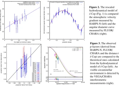
Figure 2.The rescaled

hydrodynamical model of

δCep (Fig. 1) is compared to the atmospheric velocity gradient measured by HARPS-N (left) and the angular diameter curve measured by FLUOR/ CHARA (right). 1.24 1.26 1.28 1.3 1.32 1.34 1.36

1.24 1.26 1.28 1.3 1.32 1.34 1.36

projection factor from observations

projection factor from theory line 1 line 2 line 3 line 4 line 5 line 6 line 7 line 8 line 9 line 10 line 11 line 12 line 13 line 14 line 15 line 16 line 17 0 0.2 0.4 0.6 0.8 1 square d v is ibili ti es open symbols:

model of pulsating disk + CSE solid lines: model of pulsating disk

b)

φ = 0.300

φ = 0.543 +/- 0.009

φ = 0.666 +/- 0.006

φ = 0.821 +/- 0.012

-0.2 -0.1 0 0.1 0.2

0 5e+07 1e+08 1.5e+08 2e+08

spatial frequencies in 1/rad

Figure 3.The observed

p-factors (derived from HARPS-N, FLUOR/ CHARA and the distance to

δCep) are compared to the theoretical ones calculated from the hydrodynamical model ofδCep (left). An visible circumstellar environment is detected by the VEGA/CHARA interferometric measurements (right).

Table 3 in [14]). The comparison between observed and theoretical projection factors (derived from the hydrodynamical code) are plotted in Figure 3 (left). The agreement of the hydrodynamical model with the atmospheric velocity gradient, the angular diameter curve and the individual projection fac-tors associated to specific lines, supports the decomposition of the projection factor as described in Section 2.

4 The bright visible environment of

δ

Cep revealed by VEGA/CHARA

observations

An improved BW method or SPIPS approach (with in particular well calibrated p-factors and CSEs) will provide a robust tool to derive the distance of individual Cepheids up to few Mpc in the Local Group. The problem of the metallicity dependence of distance indicators in the Local Group will be then revisited in the framework of the Araucaria Project ([22]). After a long history, the BW projection factor remains a key quantity in the calibration of the cosmic distance scale, and one century after the discovery of the period-luminosity relation, Cepheid pulsation and environment is still a distinct challenge.

Acknowledgments: The observations leading to these results have received funding from the European Commis-sion’s Seventh Framework Programme (FP7/2013-2016) under grant agreement number 312430 (OPTICON). The authors thank the CHARA Array, which is funded by the National Science Foundation through NSF grants AST-0606958 and AST-0908253 and by Georgia State University through the College of Arts and Sciences, as well as the W. M. Keck Foundation. WG gratefully acknowledges financial support for this work from the BASAL Centro de Astrofisica y Tecnologias Afines (CATA) PFB-06/2007, and from the Millenium Institute of Astrophysics (MAS) of the Iniciativa Cientifica Milenio del Ministerio de Economia, Fomento y Turismo de Chile, project IC120009. We acknowledge financial support for this work from ECOS-CONICYT grant C13U01. Support from the Polish National Science Center grant MAESTRO 2012/06/A/ST9/00269 is also acknowledged. EP and MR acknowledge financial support from PRIN INAF-2014. NN, PK, AG, and WG ac-knowledge the support of the French-Chilean exchange program ECOS-Sud/CONICYT (C13U01). The authors acknowledge the support of the French Agence Nationale de la Recherche (ANR), under grant ANR-15-CE31-0012- 01 (project UnlockCepheids) and the financial support from “Programme National de Physique Stellaire” (PNPS) of CNRS/INSU, France.

References

[1] Leavitt, H. S., & Pickering, E. C., Harvard College Observatory Circular,173, 3 (1912) [2] Riess, A. G., Macri, L. M. , Hoffmann, S. L., et al., ApJ,826, 56, (2016)

[3] Planck Collaboration, Ade, P. A. R., Aghanim, N., Arnaud, M., et al., A&A,594, 13 (2016) [4] Storm, J., Gieren, W., Fouqué, P., et al., A&A,534, 94, (2011)

[5] Storm, J., Gieren, W., Fouqué, P., et al., ApJ,534, 95, (2011) [6] Kervella, P., Nardetto N., Bersier D., et al., A&A,416, 953, (2004) [7] Mérand, A., Kervella, P., Breitfelder, J., et al., A&A,584, A80 (2015) [8] Breitfelder, J., Mérand, A., Kervella, P., et al., A&A,587, 117 (2016) [9] Kervella, P., Trahin, B., Bond, H. E., et al., A&A,600, A127 (2017)

[10] Nardetto, N., Mourard, D., Mathias, P., Fokin, A., & Gillet, D., A&A,471, 661 (2007) [11] Mérand, A., Kervella, P., Coudé du Foresto, V., et al., A&A,453, 162, (2006)

[12] Nardetto, N., Fokin, A., Mourard, D., & Mathias, P., A&A,454, 332, (2006) [13] Nardetto, N., Gieren, W., Kervella, P., et al., A&A,502, 956, (2009) [14] Nardetto, N., Poretti, E., Rainer, M., et al., A&A,597, 73, (2017)

[15] Nardetto, N., Fokin, A., Mourard, D., Mathias, P., et al., A&A,428, 137, (2004) [16] Mérand, A., Kervella, P., Coudé du Foresto, V., et al., A&A,438, 9, (2005) [17] Majaess, D., Turner, D., & Gieren, W., ApJ,747, 145, (2012)

[18] Mourard, D., Clausse, J. M., Marcotto, A., et al., A&A,508, 1083, (2009) [19] Nardetto, N., Mérand, A., Mourard, D., et al., A&A,593, 45, (2016) [20] Anderson, R. I., Sahlmann, J., Holl, B., et al., ApJ,804, 144 (2015) [21] Engle, S. G., Guinan, E. F., Harper, G. M., et al., ApJ,838, 67 (2017)