1 Title
A global sea state dataset from spaceborne synthetic aperture radar wave mode data
Authors
Xiao-Ming Li1, BingQing Huang1,2
Affiliations
1. Aerospace Information Research Institution, Chinese Academy of Sciences 2. University of Chinese Academy of Sciences
corresponding author: Xiao-Ming Li ([email protected]; [email protected])
Abstract
This dataset consists of integral sea state parameters of significant wave height (SWH)
and mean wave period (zero-upcrossing mean wave period, MWP) data derived from
the advanced synthetic aperture radar (ASAR) onboard the ENVISAT satellite over its
full life cycle (2002-2012) covering the global ocean. Both parameters are calibrated
and validated against buoy data. A cross-validation between the ASAR SWH and radar
altimeter (RA) data is also performed to ensure that the SAR-derived wave height data
are of the same quality as the RA data. These data are stored in the standard NetCDF
format, which are produced for each ASAR wave mode Level1B data provided by the
European Space Agency. This is the first time that a full sea state product in terms of
both the SWH and MWP has been derived from spaceborne SAR data over the global
ocean for a decadal temporal scale.
Background & Summary
The sea state is one of the key parameters of the “essential climate variables” (ECVs)
defined by the Global Climate Observing System (GCOS) to meet the requirements of
the climate change community. Spaceborne radar measurements of the sea state in terms
of the significant wave height (SWH) and mean wave period (MWP), particularly
Long-term RA measurements can reflect some wave height trends in the global oceans, and
these trends might be associated with climate change2. Another radar sensor capable of
measuring the sea state is known as spaceborne synthetic aperture radar (SAR), which
became available at the same time as RAs; consequently, both instruments were on
board the Seasat3 satellite launched in 1978. However, unlike nadir-looking RAs, SAR
is a side-looking radar, which allows SAR to image large surface areas. Additionally,
SAR can achieve a high spatial resolution in the azimuth (flight) direction through the
“aperture synthetizing” technique4. In principle, spaceborne SAR should be able to
effectively measure the sea state from space, as this technology images sea surface
waves in two dimensions5, at a high spatial resolution. However, as surface waves are
in motion during the SAR imaging time (i.e., water particles are moving either toward
or away from the radar system), the high-frequency components of ocean waves are
missed (the “cut-off effect”), and the distortion of the spectrum occurs during the
imaging process of SAR6-7. Therefore, the SAR imaging of surface gravity waves is
generally considered a nonlinear process8, complicating the retrieval of ocean wave
parameters from SAR data. Two-dimensional wave spectra predicted by ocean wave
modeling (e.g., WAM9) or derived from other sources10 must commonly be used as a
priori information (also called the “first guess”) in the retrieval11 to compensate for the
lost and distorted ocean wave information during SAR imaging. However, as a result
of this compensatory approach, the retrieval of ocean wave parameters from SAR data
has to rely on the priori information, which significantly limits SAR as an independent
remote sensing instrument that can measure the sea state.
The wave mode (WM), which is dedicated to measurements of ocean wave, is a
unique imaging mode of SAR. Although the WM covers a relatively small area of the
sea surface (approximately 6 km by 10 km), these data are automatically acquired by
missions (ERS-1, 1991 – 2000 and ERS-2, 1995 - 2011)12-15 to the Environment
Satellite (ENVISAT) mission (2002 – 2012)16-17 and the current Sentinel-1A/1B (2014
- )18 and the Chinese Gaofen-3 (2016 -) missions19, WM data have been available for
nearly 30 years and will continue to be acquired into the future, constituting a valuable
dataset for global sea state measurements. On the basis of SAR WM data, some
interesting investigations of global ocean waves, particularly with respect to the
characteristics of ocean swells20-22, have been reported. Such analyses can be performed
because ocean swells are generally considered linearly or quasi-linearly imaged by SAR;
thus, the abovementioned nonlinear inversion process can be “degraded” to a
quasilinear approach23-24, in which case a priori information is no longer needed.
However, such a quasilinear inversion cannot yield full sea state parameters of both
windsea (wind waves) and swell, and instead yields the sea state parameters of swell,
or more accurately called the parameters of the ocean wave components imaged by
spaceborne SAR. Therefore, to overcome such a weakness, various parametric models
that directly relate SAR-measured sea surface radar backscatter (radar cross section) to
the full sea state parameters of SWH and MWP of both windsea and swell have been
proposed14, 17-18, which also do not need a priori information and can provide
independent SAR measurements of global ocean waves. Here, we developed a global
sea state dataset from the WM data acquired by the advanced synthetic aperture radar
(ASAR) onboard the satellite ENVISAT from 2002 to 2012 based on the parametric
model “CWAVE_ENV”17. This is the first time that a global ocean dataset of full sea
state parameters in terms of both SWH and MWP in a decadal temporal scale has
become publicly available based on spaceborne SAR data and we believe that this
dataset, in conjunction with RA datasets that widely exploited at present, is valuable for
global observations of ocean waves. On the other hand, full sea state parameters also
the CWAVE type algorithms. Therefore, by combining both the historical ASAR WM
ocean wave product and the current continuously obtained Sentinel-1 WM product, one
can expect a long-term spaceborne SAR sea state dataset available for global ocean
observations. Methods
ASAR WM data. In the ERS-1 and ERS-2 missions, the SAR WM data were
publicly available in the formation of two-dimensional image spectra in discrete formats,
i.e. allocating the image spectrum energy in numbers of directional and frequency bins25.
Beginning with the ENVISAT mission, the ASAR WM data in single look complex
format26 (i.e., consisting of a real part R and an imaginary part I ) were provided to users; these data record both the magnitude and phase of the returned radar signals. The
SAR image intensity (𝐼) is therefore calculated as 𝐼 𝑅 𝐼 . By performing a radiometric calibration of intensity data, the normalized radar cross section, denoted 𝜎 , can be obtained and then used to retrieve sea state parameters.
ASAR WM data have a spatial coverage ranging from 6 km x 5 km to 10 km x 5
km over the sea surface. The distance between two consecutive acquisitions of WM
data is 100 km, which could be seen from the image geometry of ASAR WM in Figure
1(a). One example of ASAR WM data acquired over the ocean is shown in Figure 1(b),
(a) (b)
Fig. 1 (a) Geometry of the ASAR WM data acquisitions. Note the WM data with an incidence
angle of 33° acquired by ASAR were only available during experiments (refer to the main text for
details). (b)is an example of ASAR WM images acquired over the ocean. The acquisition date and
location are marked on the image.
The parametric model “CWAVE_ENV” was applied to the ASAR WM data to
generate the sea state parameters of SWH (𝐻 and MWP (𝑇 ). This type of parametric model was first proposed for the reprocessed ERS-2 WM data14; the name
“CWAVE” indicates the use of a C-band (SAR) wave retrieval algorithm, such as the
widely used C-band geophysical model function “CMOD”27, to retrieve sea surface
wind fields from scatterometer and SAR data. Because the development and validation
of parametric models have been described in detail in previous studies14,17, only the
rationale for using a parametric model is discussed here.
Although imaging mechanisms of ocean surface gravity waves by SAR remain to
be further investigated, the measured radar backscatter from the sea surface is closely
related to various sea state parameters (denoted 𝑊) through relations with a set of parameters (expressed as a vector, 𝑺 𝑠 , … , 𝑠 ). These parameters can be directly derived from SAR data, as expressed in equation 1.
𝑊 𝑎 𝑎 𝑠 𝑎, 𝑠 𝑠 (1)
In the above model, the sea state parameter 𝑊is expressed as a linear combination of a
number of 𝑛 ASAR image parameters 𝑺 𝑠 , … , 𝑠 with the extended coefficient
vector 𝑨 𝑎 , … , 𝑎 , 𝑎 , … , 𝑎 𝑎 . To also include nonlinearities as well as possible
coupling among different parameters, a quadratic term is added to the equation (the
in the CWAVE_ENV model. Two parameters of the normalized radar cross section 𝜎 and the variance 𝑐𝑣𝑎𝑟, are directly calculated from the intensity data. The remaining 20 parameters are derived from the FFT spectrum of the ASAR WM intensity image. The
major reason for using the spectral parameters is that the traditional nonlinear or
quasi-linear retrievals connect the SAR image spectrum with two-dimensional ocean wave
(or swell) spectra. On the other hand, 𝜎 is closely related with the wind speed (e.g., represented by the CMOD functions), and therefore, the information of windsea on SAR
images is also involved in this equation. This is the general rational that the function
can represent both swell and windsea information.
The least-square minimization approach is used to determine the coefficient vector
𝑨 which consists of a number of 𝑛 coefficients, as defined in equation 2, where
𝑤 , 𝑺 , … , 𝑤 , … , 𝑺 represents the available data pairs of SAR image parameters
and the collocated tuning dataset of the integral sea state parameter (e.g., SWH or
MWP).
𝐽 𝐴 𝑤 𝑨 𝑺 (2)
After the coefficient vector 𝑨 is determined, one can derive the SWH or MWP directly from ASAR WM data using equation 1. The preliminary validation of the
ASAR-derived ℎ values using the CWAVE_ENV algorithm was conducted for a two-month (January and February 2017) dataset. Comparisons with the National Data Buoy Center
(NDBC) in situ buoy measurements yielded a bias of 0.06 m and a
root-mean-squared-error (RMSE) of 0.70 m17. Here, we applied this parametric model to the entire dataset
of the ASAR WM data of its full life cycle.
The entire ENVISAT mission ranged from March 2002 to April 2012. The ASAR
December 2002 to April 2012. During the lifetime of ENVISAT, the ASAR instrument
acquired WM data in vertical-vertical (VV) polarization with an incidence angle of 23º,
except during two experimental periods, in which the acquired WM data had an
incidence angle of approximately 33º. The first period ranged from January 24th to
February 6th, 2007, and the second one ranged from March 6th to March 13th, 2007.
From January 24th to January 30th, 2007, the WM data were acquired in
horizontal-horizontal (HH) polarization. In addition to excluding the WM data acquired during
these two experimental periods, the following criteria were applied to further screen the
data.
(i) The ASAR WM data acquired in polar regions were excluded from further
processing because they might be affected by sea ice; thus, only the data acquired
between 65ºS and 70ºN were used to generate sea state parameters.
(ii) Although ASAR WM images have a relatively small spatial coverage compared
with images acquired in other modes, e.g., the imaging mode and wide swath mode, the
WM images are also affected by other sea surface features not related with ocean waves,
e.g., oil spills, atmospheric features, and bright targets. To select only ASAR WM
images that display a homogeneous sea surface (e.g., the case shown in Figure 1) and
derive sea state parameters, some parameters were used for automatic detection. We
previously used the “homogeneity factor”28 to classify ASAR WM images into
homogenous and inhomogeneous classes; if the sea surface is “purely” homogeneous,
this factor is equal to 1. Through the visual inspection of large amounts of both
ERS-2/SAR and ENVISAT/ASAR WM data, the homogeneity factor was set to 1.05 as a
threshold for selecting appropriate ASAR WM data for retrieval. Approximately 94.42%
of the data have a homogeneity factor lower than 1.05, which are treated as good data
homogeneity parameter higher than 1.05 may also present an acceptable situation of
retrieval. Therefore, we lowed the threshold of the homogeneity factor to 1.50 in order
to process more data to sea state parameters, but the data with a homogeneity factor in
the range between1.05 and 1.50 are flagged as “suspect” for further investigation, which
is described in detail in Data Records. It should be noted that only the WM data with a
homogeneity parameter 1.05 were used for calibration and validation presented in the
following. After the aforementioned preprocessing steps, approximately 6.69 million
ASAR WM data were used to generate global ocean wave parameters.
In situ buoy data. In situ buoy measurements of sea state parameters were used to
validate and calibrate the retrieved SWH and MWP based on the ASAR WM data. The
GlobWave project (http://globwave.ifremer.fr/) collected a large amount of in situ buoy
data from several buoy networks. Among the different buoy datasets, it is found that the
one provided by the European Center for Medium-Range Weather Forecasts (ECMWF)
contains more data (649 buoys collected between 2002 and 2012) than any of the other
datasets. It is a comprehensive collection of buoy data from various networks including
NDBC, the Marine Environmental Data Section (MEDS), the Coastal Data Information
Program (CDIP) and others. Therefore, we selected the ECMWF-provided buoy data
(hereafter referred to as “ECMWF buoy data”) for the evaluation and calibration of the
ASAR-derived SWH.
The ASAR-retrieved MWP is the zero-upcrossing mean wave period (𝑇 , also often denoted 𝑇 ), as defined in equation 3. One can find that both the definitions of 𝐻 and 𝑇 are in a consistent manner relating to zero-upcrossing waves. Both are the
two widely used parameters to describe sea state. We found that many recorded MWP
NDBC spectral data are normal. Therefore, we used the NDBC two-dimensional buoy
spectrum (also accessed from the GlobWave data portal, hereafter called “NDBC buoy
data”) to calculate 𝑇 for comparison with the ASAR-retrieved MWP. The quality flag of the NDBC buoy spectral data in the GlobWave data portal is named
spectral_wave_density_qc_level. The values of this flag are 0, 1, 2, 3 and 4, which
represent unknown, unprocessed, bad, suspect and good, respectively. We used only the
good wave spectral data for calibration and validation.
𝑇 𝑚 𝑚⁄ (3)
𝑚 𝑓 𝑆 ∆𝑓 (4)
In the above equations, m is the 𝑛 spectral moment, 𝑓 is the 𝑖 discrete frequency, 𝛥𝑓 is the width of the 𝑖 discrete frequency and 𝑆 is the spectral density over the 𝑖 frequency.
Both the ECMWF and NDBC buoy data were collocated with the ASAR WM data
following the criteria that the temporal difference is less than 30 minutes and the spatial
distance is less than 100 km. For cases in which several buoys satisfied the collocation
criteria, only the measurements from the buoy nearest to the corresponding ASAR WM
Fig. 2 Locations of the collocated ECMWF buoys (red squares) and NDBC buoys (green dots)
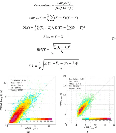
Comparison of ASAR retrievals with buoy wave data. To compare the
ASAR-derived SWH (denoted ASAR_𝐻 ) with the ECMWF buoy SWH (denoted 𝐸𝐶𝑀𝑊𝐹_𝑏𝑢𝑜𝑦_𝐻 ), we limited the SWH to the range from 0.5 m (to avoid the biased
retrievals induced by the very low radar backscatter of the sea surface) to 30.0 m.
Eventually, 29,123 data pairs were retained for comparison, and the corresponding
scatter diagram is shown in Figure 3(a). With respect to the comparison of MWP, the
NDBC buoy MWP (denoted NDBC_𝑇 )are all larger than 2.0 s but smaller than 20.0 s). Eventually, 15,393 data pairs were used for calibration and validation, and the
corresponding scatter diagram is shown in Figure 3(b). The colors in the two diagrams
indicate the density of data pairs.
The following four statistical parameters were used to evaluate the comparisons of
the ASAR-derived (referring to both raw and calibrated) sea state parameters with buoy
correlation coefficient is calculated by the covariance 𝐶𝑜𝑣 𝑋, 𝑌 and the variances 𝐷 𝑋 and𝐷 𝑌 .
𝐶𝑜𝑟𝑟𝑒𝑙𝑎𝑡𝑖𝑜𝑛 𝐶𝑜𝑣 𝑋, 𝑌 𝐷 𝑋 𝐷 𝑌
𝐶𝑜𝑣 𝑋, 𝑌 1
𝑁 𝑋𝑖 𝑋 𝑌𝑖 𝑌
𝐷 𝑋 ∑ 𝑋 𝑋 , 𝐷 𝑌 ∑ 𝑌 𝑌
𝐵𝑖𝑎𝑠 𝑌 𝑋
𝑅𝑀𝑆𝐸 ∑ 𝑌 𝑋
𝑁
𝑆. 𝐼. 1 𝑌
∑ 𝑌 𝑌 𝑋 𝑋
𝑁
(5)
(a) (b)
Fig. 3 (a) Comparison between the ASAR-derived SWH and the ECMWF buoy data. (b)
Comparison between the ASAR-derived MWP and the NDBC buoy data.
ASAR_𝐻 is slightly higher than ECMWF_buoy_𝐻 with a bias of 0.07 m. The
RMSE is 0.62 m, which is close to the result (0.70 m) achieved in the preliminary
validation based on a two-month dataset17. The scatter index (S.I.) of 25.68% is
retrievals are also slightly higher than the NDBC buoy-measured periods with a bias of
0.21 s. In contrast, the retrieved ASAR_𝑇 are closely distributed both sides of the 1:1 diagonal line, and therefore, the comparison yields a low S.I. of 12.36%. With respect
to the correlation coefficient, both comparisons suggest that the ASAR retrievals
display good agreement with the ECMWF and NDBC buoy measurements, having
values of 0.89 and 0.83, respectively.
Calibration of the ASAR-derived SWH data. Our goal is to calibrate the
ASAR-derived sea state parameters using buoy measurements; however, quite a few
collocations are outliers, as illustrated in Figure 3. If these outliers are included in the
calibration process, they can introduce uncertainty. Therefore, we used quartiles to
exclude some outliers from the calibration process29. Quartiles are obtained by dividing
the data sorted into ascending order into four equal groups, which can be used to
describe the distribution of the data and identify the outliers. The second quartile 𝑄 is the median of the data. The first quartile 𝑄 and the third quartile 𝑄 represent the data between the median and the minimum and maximum, respectively. 𝐼𝑄𝑅 is the
interquartile range. According to 𝑄 ,𝑄 , 𝑄 and the 𝐼𝑄𝑅, the lower and upper bounds can be calculated. The data exceeding the lower and upper fences are regarded as
outliers.
𝐼𝑄𝑅 𝑄 𝑄
𝑙𝑜𝑤𝑒𝑟 𝑏𝑜𝑢𝑛𝑑 𝑄 1.5𝐼𝑄𝑅
𝑈𝑝𝑝𝑒𝑟 𝑏𝑜𝑢𝑛𝑑 𝑄 1.5𝐼𝑄𝑅
(6)
By applying these quartiles to exclude some outliers, which is based on statistical
analysis of the collocated data, we further employed robust regression to detect the
outliers30,31 of the collocated data pairs. Robust regressionis a linear regression method
weights. By applying least-square minimization, the predicted values and residuals are
calculated, where the residuals represent the difference between the predicted values
and the observed ones. The data with large residuals are assigned small weights in the
subsequent iterations. After a few iterations, the weights of the fitting data are adjusted,
and the outliers are verified to have small weights. In this study, the fitting data with
weights smaller 0.15 are considered outliers and are excluded from the calibration of
the ASAR SWH data.
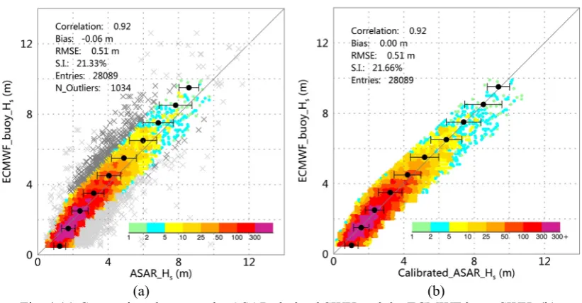
The light and dark gray cross symbols in Figure 4 represent the outliers detected by
the quantile and the robust regression methods, respectively.
(a) (b)
Fig. 4 (a) Comparison between the ASAR-derived SWH and the ECMWF buoy SWH. (b)
Comparison between ASAR-derived SWH and the ECMWF buoy SWH after calibration. The
light and dark gray cross symbols are the outliers detected by quantile and robust regression
methods, respectively.
Although the quantile and robust regression methods successfully excluded some
data pairs as outliers (as indicted by the improved statistical parameters), the
increases along with sea state varying. In the next step, the buoy measurements were
used to calibrate the ASAR retrievals.
The in situ measurements are the most appropriate data source of Cal/Val of
satellite retrievals. However, these data are not completely unbiased or free of errors32.
Therefore, we used the reduced major axis (RMA) regression method 31,33, which treats
the variables 𝑥 (ASAR_𝐻 ) and 𝑦 (ECMWF_buoy_𝐻 ) independently, to calibrate the ASAR retrievals. In the regression, the errors of 𝑥 and 𝑦 are both considered by
minimizing the triangular area 0.5 ∆𝑥∆𝑦 between the data points and the regression line, where ∆𝑥 and ∆𝑦 are the distances between the actual and predicted values in the 𝑥 and 𝑦 directions, respectively. By applying RMA regression to the collocated data
pairs, the following linear calibration formula for the ASAR SWH data is obtained:
𝐶𝑎𝑙𝑖𝑏𝑟𝑎𝑡𝑒𝑑_𝐴𝑆𝐴𝑅_𝐻 𝑚 1.140 𝐴𝑆𝐴𝑅_𝐻 𝑚 0.402 (7)
Figure 4(b) shows a comparison between the Calibrated_ASAR_𝐻 and the buoy measurements ECMWF_buoy_𝐻 . The calibration process does improve the bias, which decreases from 0.06 m to zero. However, the other three parameters, including the
correlation coefficient, RMSE and S.I., do not improve. Although performing the
calibration does not improve the overall statistical parameters, it significantly improves
the underestimation of the ASAR-retrieved SWH, as revealed by the error bars overlaid
on the scatter diagram, while the underestimation trend originally increases with the
wave height. Because the collocated data pairs are unequally distributed among
different wave heights and much of the data (62.58%) are associated with a low to
moderate sea state (SWH< 2.5 m), the overall statistical parameters do not reflect the
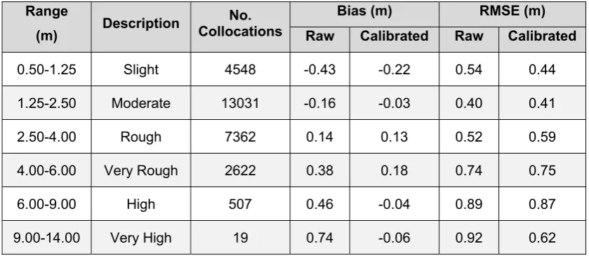
table 1 lists the variations in the bias and RMSE with the sea state (the Douglas sea
scale is used) before and after applying the RMA calibration to the collocated data pairs.
The bias is significantly reduced by the calibration process, particularly for the
slight, and higher than rough sea states. This finding indicates that the linear calibration
partially reduces the problem of overestimation for slight to moderate sea states and
underestimation for rough and high sea states. The RMSE displays slight fluctuations
before and after the calibration process, except for the very high sea state (SWH larger
than 9.00 m), for which it is reduced by approximately 33% after the calibration.
Table 1 Variations in the bias (Buoy – ASAR) and RMSE with the sea state before
and after the RMA calibration
Range
(m) Description
No. Collocations
Bias (m) RMSE (m)
Raw Calibrated Raw Calibrated
0.50-1.25 Slight 4548 -0.43 -0.22 0.54 0.44
1.25-2.50 Moderate 13031 -0.16 -0.03 0.40 0.41
2.50-4.00 Rough 7362 0.14 0.13 0.52 0.59
4.00-6.00 Very Rough 2622 0.38 0.18 0.74 0.75
6.00-9.00 High 507 0.46 -0.04 0.89 0.87
9.00-14.00 Very High 19 0.74 -0.06 0.92 0.62
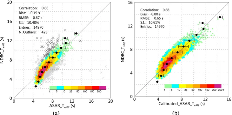
Calibration of the ASAR-derived MWP. Following the same calibration
method applied to the SWH, the NDBC buoy data are used to calibrate the
ASAR-derived MWP. In total, 15,393 data pairs were collected to calibrate the MWP data
considering the collocation criteria mentioned above. After elimination of outliers by
the quartile and robust regression methods, 14,970 pairs of data remained. The scatter
density of data pairs and the cross symbols indicate the detected outliers. Using the
RMA regression method, a linear calibration of the MWP is derived:
𝐶𝑎𝑙𝑖𝑏𝑟𝑎𝑡𝑒𝑑_𝐴𝑆𝐴𝑅_𝑇 𝑠 1.268 𝐴𝑆𝐴𝑅_𝑇 𝑠 1.887 (8)
The calibrated ASAR MWP results are plotted against the NDBC buoy data in
Figure 5(b). Comparing Figure 5 (a) with (b), the calibration improves both the bias and
the RMSE, which decrease from -0.19 s to zero and from 0.67 s to 0.65 s, respectively.
However, the correlation coefficient and S.I. do not improve. The raw data suggest that
the ASAR-derived results overestimate the MWP below 7 s but underestimate it above
8 s. The calibration makes the data pairs almost symmetrically distributed about the 1:1
diagonal line and partially corrects the trend result.
(a) (b)
Fig. 5 (a) Scatter diagram of the comparison between the ASAR-derived MWP and the NDBC buoy
MWP. (b) the same as (a) but for the comparison of the calibrated ASAR-derived MWP. There are
few data pairs with large values of MWP that are detected outliers (lower right of (a)); therefore, the
maximum value of the axes in (b) is reduced to 16 s to better visualize the distribution of the error
bars. The cross symbols in (a) are the detected outliers using the IQR (light gray) and robust regress
The above-described calibration of the ASAR retrieval is based on collocating buoy
data within a 100 km distance. We also tried to reduce the collocation distance to 50 km
(consequently, the number of collocation data pairs decreased to 8,046), which yields
the following two calibration formulas for the SWH and MWP, respectively, using the
same method described above.
𝐶𝑎𝑙𝑖𝑏𝑟𝑎𝑡𝑒𝑑_𝐴𝑆𝐴𝑅_𝐻 𝑚 1.132 𝐴𝑆𝐴𝑅_𝐻 𝑚 0.383 (9)
𝐶𝑎𝑙𝑖𝑏𝑟𝑎𝑡𝑒𝑑_𝐴𝑆𝐴𝑅_𝑇 𝑠 1.256 𝐴𝑆𝐴𝑅_𝑇 𝑠 1.821 (10)
The difference in the formulas derived based on a100 km and 50 km collocation
distance for calibrating the ASAR-derived SWH and MWP is nearly neglected. For
instance, assuming an extreme sea state with the SWH of 20 m, the difference in the
calibrated SWH using the two formulas is approximately 0.14 m, which accounts for
0.7% of the SWH. In the provided product, the derived calibration formulas based on a
100 km collocation distance are applied to the ASAR retrieval of SWH and MWP, while
the user can easily apply the other set of calibration formulas in (9) and (10) for
exploitation.
Data records
The ASAR WM data global wave product is stored in NetCDF-3 format and follows
the Climate and Forecast Metadata CF-1.7 convention34. The naming convention of the
ASAR sea state product files is as follows:
Satid_Sensor_Type_StartDate_StartTime_EndDate_EndTime_Cycle_Orbit.NC,
where
b. Sensor: sensor name
c. Type: type of product
d. StartDate: Date of the first record e. StartTime: Time of the first record f. EndDate: Date of the last record g. EndTime: Time of the last record h. Cycle: cycle number of the satellite
i. Orbit: relative orbit number of the satellite
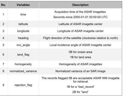
The records contained in the product correspond to the imagettes of the ASAR WVI
Level 1B product. Each record consists of 14 variables, which are listed in the following
table 2.
Table 2 List of variables and their descriptions in the ASAR WM sea state NetCDF
product
No. Variables Description
1 time Acquisition time of the ASAR imagettes.
Seconds since 2000-01-01 00:00:00 UTC
2 latitude Latitude of ASAR imagette center
3 longitude Longitude of ASAR imagette center
4 heading Flight direction of the satellite (clockwise relative to north)
5 inci_angle Local incidence angle of ASAR imagette center
6 land_flag 0B for ocean area
1B for land area
7 homogeneity Homogeneity of ASAR imagettes
8 normalized_variance Normalized variance of an SAR image
9 rejection_flag
The records flagged 0B are acceptable ASAR WM imagette for retrieval
3B for “inhomogeneous ASAR imagettes” 4B for “ASAR imagettes in HH polarization”
5B for “ASAR imagettes with an incidence angle not equal to 23°”
6B for “ASAR imagettes in polar regions, i.e. beyond 70°N or 65°S”
10 qc_flag
0B for a good record 1B for a suspect record
2B for a bad record
11 swh Retrieved SWH of ASAR imagettes
12 mwp Retrieved zero-upcrossing wave period of ASAR imagettes
13 swh_cali Calibrated SWH
14 mwp_cali Calibrated zero-upcrossing MWP
The “swh” and “mwp” are the retrieved sea state parameters using the
CWAVE_ENV model. By applying the calibration formulas given in equations 7 and
8, the calibrated ASAR-derived SWH and MWP are obtained and stored as the variables
“swh_cali” and “mwp_cali”.
The diagram shown in Fig. 6 illustrates the structure of the “rejection_flag” and
Fig. 6 Structure of the “rejection_flag” and “qc_flag” of the developed global ASAR WM wave
products.
The “rejection_Flag” flags mark the ASAR WM records with values of 0, 1, 2, 3,
4, 5 or 6, which represent an acceptable ASAR WM imagette for retrieval, a bad record
(identified in reading the Level 1B data), a record containing land (discrimination is
based on “land_flag”), an inhomogeneous (homogeneity factor > 1.5) ASAR imagette,
an imagette acquired in HH polarization, an imagette with an incidence angle not equal
to 23°, and an imagette acquired in the polar regions, respectively. The “land_flag” is
inherited from the ASAR WM Level 1B data, i.e., each imagette in the Level 1B data
has been flagged “land” or not. The “normalized_variance”25 variable is the normalized
variance of the ASAR WM intensity data and is calculated according to equation 9.
𝑛𝑜𝑟𝑎𝑚𝑎𝑙𝑖𝑧𝑒𝑑_𝑣𝑎𝑟𝑖𝑎𝑛𝑐𝑒 𝐼
𝐼 𝐼
𝐼 ∑ 𝐼,
, ,
𝑀 𝑁
𝐼 ∑ 𝐼, 𝐼
, ,
𝑀 𝑁
(9)
where 𝐼 and 𝐼 represent the variance and mean of the image, respectively, and 𝑀 and 𝑁 refer to the width and height of the image, respectively.
The “qc_flag” variable has three values that describe the quality of the retrieved
sea state parameters. We considered a few factors during the quality control process,
including the reasonable range of retrievals, the normalized variance of the original
ASAR intensity image and the “rejection_flag”. Based on the factors, the records were
(1) Good record (qc_flag = 0B), which satisfies the following criteria:
a. 0 m ≤swh (swh_cali) < 30 m and 0 s < mwp (mwp_cali) < 20 s
b. σ -NESZ > 3 dB
c. rejection_flag = 0B
where σ is the mean normalized radar cross section of the ASAR imagettes and NESZ is the noise equivalent sigma zero, i.e., the noise floor of the ASAR WM data.
(2) Suspect record (qc_flag = 1B), which satisfies the following criterion:
a. swh > 30 m or mwp > 20 s
b. 1.05 ≤ homogeneity factor≤ 1.5
Among the ASAR collocations with buoy data, there are 1,416 data pairs with
homogeneity factors between 1.05 and 1.50. Their comparison with the ECMWF buoy
SWH has a bias of -0.26 m, an RMSE of 1.02 m, and a correlation of 0.63. Although
these statistical parameters are obviously worse than the comparison achieved using the
ASAR WM data with homogeneity factors less than 1.05 (Figure 3(a)), a large portion
of these data still have good consistency with the buoy measurements. If the collocation
data pairs with homogeneity factors larger than 1.50 (the amount is 677) are compared
with the ECMWF buoy SWH, a correlation of only 0.31 and a large S.I. of 79.20% are
found. Therefore, we assign the “qc_flag” of the ASAR retrievals with homogeneity
factors between 1.05 and 1.50 to “suspect”, indicating that these records require further
investigation.
a. swh (swh_cali) < 0 m or mwp (mwp_cali) < 0 s
b. σ -NESZ ≤ 3 dB
Any record with the variable “rejection_flag” not equal to 0B is excluded from further
processing, and the “qc_flag” is therefore set to “_Fillvalue”.
Each ASAR WM Level 1B data with a filename extension of “.N1” that we
received from the ESA is processed to an NC record. All the NC records in the same
year are compressed to a single file with the file extension “.tar.gz”; therefore, there are
together 11 GNU zip files corresponding to the data from the year 2002 to 2012. They
have been uploaded to the public repository Sea Scientific open data publication
(SEANOE, https://www.seanoe.org) with full free access35.
Technical validation
Comparison with RA wave data. The GlobWave project also collected wind and
wave data for the Geodetic Satellite (GEOSAT), GEOSAT Follow-on (GFO), ERS-1,
ERS-2, TOPEX/POSEIDON, JASON-1, JASON-2 and CryoSAT-2 RA missions, with
a time span from 1985 onwards. The JASON-1 mission provided wave data from
December 2001 until July 2013, which covers the lifetime of the ASAR instrument.
GlobWave reprocessed the original JASON-1 measurements and provided quality
control flags and calibrated SWH measurements. In this study, we used calibrated
Ku-band SWH measurements of JASON-1 to perform a cross-validation with the calibrated
ASAR-derived SWH. A quality flag named “swh_quality” provided in the GlobWave
RA products is used to filter the JASON-1 SWH data with high quality for validation.
This flag has three values, namely, 0, 1, and 2, representing a “good_measurement”,
“acceptable_for_some_applications” and “bad_measurement”, respectively. Only the
criteria employed in the collocation of buoy data were utilized between the ASAR data
and the JASON-1 data.
Following the same criteria of collocating the ASAR with buoy, 46,642 data pairs
of JASON-1 and ASAR WM data were obtained. However, a large number of SWH
measurements from JASON-1 of the GlobWave product in 2012 were abnormal,
ranging from -40 m to 40 m and exhibiting a discontinuous spatial distribution. The data
in 2012 were discarded from the validation dataset. In addition, we set a valid range of
SWH from 0.5 m to 30 m for validation. Finally, 23,192 pairs of JASON-1 and ASAR
WM data were obtained. Using the quartile method described above to exclude outliers,
22,880 pairs of data were collected for validation. As there are only few data available
for SWH above 10 m, the quartile method of detecting outliers does not function in that
range. However, we retain them for comparison. Figure 7(a) shows the comparison
between the ASAR-derived SWH and JASON-1 SWH (denoted JASON1_H ). The robust regression method was not applied to exclude outliers because we consider both
datasets to comprise independent measurements. The calibrated ASAR SWH (applying
equation 7) is also compared with the JASON-1 calibrated SWH35
(Calibrated_JASON1_H ), as shown in Figure 7(b).
As shown in Figure 7(a), the ASAR SWH displays good consistency with the
JASON-1 SWH, and the bias and RMSE are 0.04 m and 0.48 m, respectively;
additionally, the correlation coefficient and S.I. are 0.93 and 16.84%, respectively.
Although the ASAR SWH is generally slightly lower than the JASON-1 SWH, it is
higher for a relatively low sea state (SWH < 2.5 m). In Figure 7(b), the calibrated ASAR
SWH also displays good agreement with the calibrated JASON-1 SWH, with bias,
RMSE, correlation coefficient and S.I. values of 0.18 m, 0.53 m, 0.93 and 16.64%,
underestimation of ASAR-derived SWH is significantly improved after the calibration
process, particularly for SWH above 6 m.
(a) (b)
(c) (d)
Fig. 7 (a) and (c) Comparison between the ASAR-derived SWH and the RA SWH along with the
corresponding Q-Q plot, respectively. (b) and (d) Comparison between the calibrated ASAR-derived
SWH and the calibrated RA SWH along with the corresponding Q-Q plot, respectively.
A major limitation of these overall comparisons in evaluating the retrieval of sea
state parameters is that the data pairs are unevenly distributed among different sea states.
As the sea state increases in severity, the number of valid data pairs decreases. Therefore,
a stepwise comparison was conducted to assess the performance of the ASAR SWH
ASAR SWH compared with the JASON-1 SWH at a 1-m interval. Figure 8 (b) is the
same as (a) but compares the ASAR SWH with the calibrated JASON-1 SWH.
(a) (b)
Fig. 8 Variations in the bias and RMSE of the ASAR-derived SWH versus the JASON-1 SWH (a)
and the calibrated JASON-1 SWH (b).
Due to the changes in the bias and RMSE illuminated in Figure 8(a) and (b)
showing similar trends, we use Figure 8(a) as an example. Figure 8(a) shows the
changes in the bias and RMSE of the uncalibrated and calibrated ASAR SWH versus
the JASON-1 SWH, where the blue and red lines represent the bias and RMSE,
respectively and the solid and dashed lines refer to the uncalibrated and calibrated
ASAR SWH, respectively. The bias of the uncalibrated ASAR SWH increases with the
sea state and changes from negative to positive when the SWH is approximately 2 m.
The calibration process significantly reduces the bias to less than 0.15 - 0.2 m from low
to high sea states (at approximately 8 m), and importantly, the bias becomes less
dependent on the sea state increasing. For a very high sea state (SWH>9 m), the bias
accounts for approximately 10% of the total SWH; additionally, the RMSE of the
calibrated ASAR SWH varies from 0.25 m to 1.20 m and is particularly reduced for sea
states higher than very rough (above approximately 5 m).
The cross-validation of the ASAR-derived SWH is based on the comparison with
the GlobWave JASON-1 data mainly due to that the JASON-1 RA wave data has almost
the same temporal coverage as the ASAR WM data in full-life time. Cross-validations
with other RA data remain further investigation, e.g., using the recently released
comprehensive RA dataset by Ribal and Young1, in which there are a few RA missions
that also have overlap with the operating period of the ASAR. This can particularly
diagnose the accuracy of the ASAR SWH of high sea state, as found in Figure 7.
Thus far, there is no other high-quality MWP dataset by spaceborne remote sensing
available for cross-validation of the ASAR-derived MWP. Further investigation by
carefully selecting a reanalysis wave model dataset might be worth trying.
Code availability
Both the MATLAB code script named read_AGWD.m and the IDL code named
read_AGWD.pro for reading the ocean wave parameter products are provided as
supplementary material 1 and 2, respectively.
Acknowledgments
The first author would like to thank Dr. Susanne Lehner and Dr. Johannes
Schulz-Stellenfleth, my supervisor and former colleague for their supports to develop the
CWAVE_ENV parametric model for the ASAR wave mode data. We particularly thank
the ESA for agreeing to deliver us the entire ASAR wave mode dataset under the
framework of the “Dragon 4 program”. Mr. Jean-Francois Piollo from Ifremer/Cersat
gave us the cordial help of delivering these wave mode data. Dr. Alexis Mouche, also
from Ifremer/Cersat, encouraged us to participate the ESA sea state CCI project. This
is one of our motivations to reprocess the entire ASAR WM dataset for times to standard
ocean wave products. The study is partially supported by the National Key Research
Author Contributions
X.L. initiated, designed and implemented the project and performed the bulk of the
work creating the dataset, conducting the evaluations and writing the paper. B.H.
worked on the software to produce the products and performed the calibration and
validation tasks. She also contributed to drafting the manuscript.
Competing interests
The authors declare no competing interests.
References
1. Ribal, A. & Young, I. R. 33 years of globally calibrated wave height and wind speed data based on altimeter observations. Scientific Data. 6, 1-15 (2019)
2. Young, I. R., Zieger, S., & Babanin, A. V. Global trends in wind speed and wave height.
Science. 332, 451-455 (2011),
3. Brown, W. M. & Procello, C. J. An introduction to synthetic aperture radar, IEEE spectrum. 6, 57-62 (1969).
4. Born, G. H., Dunne, J.A. & Lame, D. B. Seasat mission overview, Science. 204, 1405 – 1406 (1979)
5. McLeish, W., Ross, D., Shuchman, R. A., Teleki, P. G., Hsiao, S. V., Shemdin, O. H., & Brown, W. E. Synthetic Aperture Radar imaging of ocean waves: Comparison with wave measurements. J. Geophys. Res.85, 5003– 5011 (1980).
6. Alpers, W. & Rufenach, C. L. The effect of orbital motions of Synthetic Aperture Radar imagery of ocean waves. IEEE transactions on Antennas and Propagation. 27, 685–690 (1979).
7. Hasselmann, K., Raney, R. K., Plant, W. J., Alpers, W., Shuchman, R. A., Lyzenga, D. R., Rufenach, C. L., & Tucker, M. J., Theory of Synthetic Aperture Radar ocean imaging: A MARSEN view. J. Geophys. Res.90, 4659– 4686 (1985).
8. Hasselmann, K. & Hasselmann, S. On the nonlinear mapping of an ocean wave spectrum into a synthetic aperture radar image spectrum. J. Geophys. Res.96, 10713-10729 (1991). 9. WAMDI GROUP. The WAM model a third generation ocean wave prediction model. J.
Phys. Oceanogry.18, 1775-1810 (1984).
10. Mastenbroek, C. & de Valk, C. A semi-parametric algorithm to retrieve ocean wave spectra from synthetic aperture radar. J. Geophys. Res.105, 3497-3516 (1998).
11. Hasselmann, S., Brüning, C., Hasselmann, K., & Heimbach, P. An improved algorithm for the retrieval of ocean wave spectra from synthetic aperture radar image spectra. J. Geophys. Res.101, 16615– 16629 (1996).
12. Kerbaol, V., Chapron, B. & Vachon, P. W. Analysis of ERS-1/2 synthetic aperture radar wave mode imagettes. J. Geophys. Res.103, 7833–7846 (1998).
13. Lehner, S., Schulz-Stellenfleth, J., Schättler, J. B., Breit, H. & Horstmann, J. Wind and wave measurements using complex ERS-2 wave mode data. IEEE Trans. Geosci., and Rem. Sens.38, 2246-2257 (2000).
14. Schulz-Stellenfleth, J., König, Th. & Lehner, S. An empirical approach for the retrieval of integral ocean wave parameters from synthetic aperture radar data. J. Geophys. Res. 112,
(2007).
15. Hasselmann, K. et al. The ERS SAR wave mode: a breakthrough in global ocean wave observations. ESA special publication.SP-1326, 167-197, (2012).
Journal of Remote Sensing. 31, 4969-4993 (2010).
17. Li, X. M., Lehner, S. & Bruns, T. Ocean wave integral parameter measurements using Envisat ASAR wave mode Data. IEEE Trans. Geosci. Remote Sens.49, 155-174 (2011). 18. Stopa, J. E. & A. Mouche. Significant wave heights from Sentinel-1 SAR: Validation and
applications. J. Geophys. Res. 122, 1827-1848 (2017).
19. Li, X. M., Zhang, T. Y., Huang, B. Q., & Jia, T. Capabilities of Chinese Gaofen-3 synthetic aperture radar in selected topics for coastal and ocean observations. Remote Sens. 10, 1-22 (2018).
20. Ardhuin, F., Chapron, B. & Collard, F. Observation of swell dissipation across oceans.
Geophys. Res. Lett. 36, L06607, (2009).
21. Collard, F., Ardhuin, F. & Chapron, B. Monitoring and analysis of ocean swell fields from space: New methods for routine observations. J. Geophys. Res.114, C07023 (2009). 22. Li, X. M. A new insight from space into swell propagation and crossing in the global oceans.
Geophys. Res. Lett.43, 5202-5209 (2016).
23. Chapron, B., Johnson, H. & Garello, R. Wave and wind retrieval from SAR images of the ocean, Ann. Telecommun. 56, 682−699 (2001).
24. Engen, G. & Johnson, H. SAR-ocean wave inversion using image cross spectra. IEEE Trans. Geosci. Remote Sens.33, 329–360 (2000).
25. Brooker, G. UWA processing algorithm specification. version 2.0, Tech. Rep., ESA, ESTEC/NWP, Noordwijk, The Netherland, 1995.
26. European Space Agency, ENVISAT ASAR Product Handbook, Issue 2.2, 2007.
27. Stoffelen, A. & Anderson, D. Scatterometer data interpretation: Estimation and validation of the transfer function CMOD4. J. Geophys. Res.102, 5767– 5780 (1997).
28. Schulz-Stellenfleth, J. & Lehner, S. Measurement of 2-D sea surface elevation fields using complex Synthetic Aperture Radar data. IEEE Trans. Geosci., & Rem. Sens.42, 1149-1160 (2004).
29. Tukey, J. Exploratory Data Analysis. (Addison-Wesley. 1977)
30. Rousseeuw, P. & Leroy, A. Robust Regression and Outlier Detection 3rd edn (John Wiley & Sons, 1996)
31. Zieger, S., Vinoth, J., & Young, I. R. Joint calibration of multiplatform altimeter measurements of wind speed and wave height over the past 20 years. Journal of Atmospheric and Oceanic Technology. 26, 2549-2564 (2009).
32. Stoffelen, A. Toward the true near-surface wind speed: Error modeling and calibration using triple collocation. J. Geophys. Res. 103, 7755–7766 (1998).
33. Trauth, M. MATLAB Recipes for Earth Sciences. 4th Edn (Springer, 2015)
34. Eaton, B., Gregory, J. & Bod Drach etc. NetCDF Climate and Forecast (CF) Metadata Convebtions Version 1.7.
35. Li, X.-M. & Huang, B.Q. A global sea state dataset from spaceborne synthetic aperture radar wave mode data. SEANOE. https://doi.org/10.17882/71337 (2020).