Pattern Extraction, Classification and Comparison
Between Attribute Selection Measures
Subrata Pramanik, Md. Rashedul Islam, Md. Jamal Uddin Department of Computer Science & Engineering, University of Rajshahi
Rajshahi-6205, Bangladesh
Abstract— In this research, we have compared three different attribute selection measures algorithms. We have used ID3 algorithm, C4.5 algorithm and CART algorithm. All these algorithms are decision tree based algorithm. We have got the accuracy of three different algorithms and we observed that the accuracy of ID3 algorithm is greater than C4.5 algorithm. But the accuracy of CART algorithm is greater than other two algorithms. We have also calculated the time complexity of three different algorithms. To compare these algorithms, we have used heart disease dataset which is collected from UCI machine learning repository.
Keywords
—
Pattern extraction, Classification, Decision Tree, ID3 algorithm, C4.5 algorithm, CART algorithm.I. INTRODUCTION
Today’s world is a digital world. As the world population is increasing rapidly, the need and usage of storing enormous amount of wide ranges of data into databases have increased rapidly in recent years. Data-mining is necessary to extract hidden useful knowledge from large datasets in a given application. This usefulness relates to the user goal, in other words only the user can determine whether the resulting knowledge answers his goal.
Data mining refers to extracting or mining knowledge from large amounts of data. There are several tools of data mining. It is necessary to choose useful data mining tools to acquire useful knowledge. Also data mining tools should be highly interactive and participatory.
Decision tree induction is a greedy algorithm that constructs decision tree in a top-down recursive divide-and-conquer manner. A decision tree is a tree in which each branch node represents a choice between a numbers of alternatives, and each leaf node represents a decision. For extracting rules, information gain measure is used to select the test attribute at each node in the tree.
Classification is one of the most popular tasks in data mining. Classification involves the assignment of an object to one of several pre-specified categories. Classification of data without any interpretation of the underlying model could reduce the trust of users in the system.
Data mining is a very demanding research field among researchers now-a-days. In our research we have performed Pattern extraction, classification and comparison between
Attribute selection measures. We found that some research has been done in this field before, but their accuracy not good enough and there are spaces where improvement can be achieved.
II. OVERVIEW OF THIS WORK
At first, we have divided the data set into five fold by using five fold cross validation method. By applying five fold cross validation method, we get five fold training and testing dataset which is shown in Fig. 1.
Fig. 1 Steps for getting Training and Testing Dataset
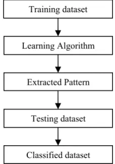
Then a classification algorithm is applied to the training dataset to extract pattern. The extracted pattern is applied to the testing dataset. Then we get the classified dataset which is shown in Fig. 2.
Fig. 2 Basic steps of this work
Data set
Five Fold Cross Validation Method
Training and Testing Data Set
Training dataset
Learning Algorithm
Extracted Pattern
Testing dataset
III.PATTERN EXTRACTION
By analyzing a large amount of data a pattern or rule is extracted. Rules are the verbal equivalent of a graphical decision tree, which specifies class membership based on the hierarchical sequence of decisions. Each rule in a set of decision rules therefore generally takes the form of a Horn clause wherein class membership is implied by a conjunction of contingent observation [1]. A typical rule structure is given below: i n 2 1 class = CLASS THEN condition AND … … AND condition AND condition IF
IV.CLASSIFICATION
Data classification is two-step process [1, 2]. In the first step, a classifier is built describing a predetermined set of data classes or concepts. This is the learning step (or training phase), where a classification algorithm builds the classifier by analyzing or “learning from” a training set made up of database tuples and their associated class labels. A tuple, X, is represented by an n-dimensional attribute vector, X=(x1,x2,……xN), depicting N measurements made on the tuple from N database attributes respectively, A1,A2…..AN. Each tuple, X, assumed to belong to a predefined class as determined by another database attribute called the class label attribute. The class label attribute is discrete-valued and unordered. It is categorical in that each value serves as a category or class. The individual tuples making up the training set are referred to as training tuples and are selected from the database under analysis. In this context of classification, data tuples can be referred to as samples, examples, instances, data points or objects [1].
Because the class label of each training tuple is provided, this step is also known as supervised learning (i.e. the learning of the classifier is “supervised” in that it is told to which class each training tuple belongs). It constructs with unsupervised learning (or clustering), in which the class label of each training tuple is not known, and the number or classes to be learned may not be known in advance [1, 2].
V. ATTRIBUTE SELECTION MEASURES
There are many algorithms to select the attribute which decides which attribute will be the top of the tree. In this research, we have used the following attribute selection measures:
A. ID3 (Iterative Dichotomiser) Algorithm
The ID3 technique [1, 2, 9] to building a decision tree is based on information theory and attempts to minimize the expected number of comparisons. The basic idea of the induction algorithm is to ask questions whose answers provide the most information. The first question divides the search space into two large search domains, while the second performs little division of the space. The basic strategy used by ID3 is to choose splitting attributes with the highest information gain first. The amount of information associated with an attribute value is related to the probability of occurrence.
Let node N represents or hold the tuples of partition D. The attribute with the highest information gain is chosen as the splitting attribute for node N. This attribute minimizes the
information needed to classify the tuples in the resulting partitions and reflects the least randomness or “impurity” in these partitions.
To calculate the gain [1, 2, 9] of an attribute, at first we calculate the entropy of that attribute by the following formula:
i n i i p p S Entropy 2 1 log ) (
(1)
where,
p
i is the probability that an arbitrary tuple in S belongs to class Ci and estimated by| |
| | ,
D
CiD . A log function
to the base 2 is used, because the information is encoded in bits. Entropy(S) is just the average amount of information needed to identify the class label of the tuple in S.
Now gain of an attribute is calculated by the formula: [1]
) ( | | | | ) ( 1 i n i i
A Entropy S
S S S
Info
(2)
where,
S
i={S1,S2,... Sn}= partitions of S according to values of attribute An = number of attributes A
|
S
i| = number of cases in the partitionS
i |S| = total number of cases in SInformation gain is defined as the difference between the original information requirement and new requirement. That is, [1] ) ( ) ( )
(A Entropy S Info S
Gain A (3)
In other words, Gain(A) tell us how much would be gained by branching on A. It is the expected reduction in the information requirement caused by knowing the value of A. The attribute A with highest information gain is chosen as the splitting attribute at node N.
B. C4.5 Algorithm
The C4.5 algorithmis Quinlan’s [1, 2, 7, 8] extension of his own ID3 algorithm for generating decision trees. Just as with CART, the C4.5 algorithm recursively visits each decision node, selecting the optimal split, until no further splits are possible.
The steps of C4.5 algorithm [1, 2, 7] for growing a decision tree is given below:
− choose attribute for root node.
− Create branch for each value of that attribute
− Split cases according to branches
− Repeat process for each branch until all cases in the branch have the same class
A question that, how an attribute is chosen as a root node? At first, we calculate of the gain ratio of each attribute. The root node will be that attribute whose gain ratio is maximum. Gain ratio is calculated by the formula: [7, 8]
) ( ) ( ) ( A SplitInfo A Gain A GainRatio (4)
splitting attribute. This attribute minimizes the information needed to classify the tuples in the resulting partitions. Such an approach minimizes the expected number of tests needed to classify a given tuple and guarantees that a simple tree if found.
To calculate the gain of an attribute, at first we calculate the entropy of that attribute by the following formula: [7, 8]
i n i i p p S Entropy 2 1 log ) (
(5)
where,
i
P is the probability that an arbitrary tuple in S belongs to class
i
C and estimated by |Ci,D |
/|D|. A log
function to the base 2 is used, because the information is encoded in bits. Entropy(S) is just the average amount of information needed to identify the class label of the tuple in SNow gain of an attribute is calculated by the formula: [7, 8]
) ( | | | | ) ( ) ( 1 i n i
i Entropy S
S S S Entropy A Gain
(6)
where,
S
i={S1,S2,... Sn}= partitions of S according to values of attribute An = number of attributes A.
|Si| = number of cases in the partition Si |S| = total number of cases in S
The gain ratio divides the gain by the evaluated split information. This penalizes splits with many outcomes. [7, 8]
| | | | log | | | | ) ( 1 S Si S Si A SplitInfo i n i
(7)
The split information is the weighted average calculation of the information using the proportion of cases which are passed to each child. When there are cases with unknown outcomes on the split attribute, the split information treats this as an additional split direction. This is done to penalize splits which are made using cases with missing values. After finding the best split, the tree continues to be grown recursively using the same process.
C. CART Algorithm
The CART algorithm [1, 2] measures the impurity of D, a data partition or set of training tuples, as
m i i P D Gini 1 2 1 )( (8)
where, Pi is the probability that a tuple in D belongs to class Ci and is estimated by |Ci,D|/|D|. The sum is computed
over m classes.
The CART algorithm [1, 2] considers a binary split for each attribute. Let’s first consider the case where A is a discrete valued attribute having v distinct values, {
a
1,a
2,...
.
a
v }, occurring in D. To determine the best split on A, we examine all of the possible subsets that can be formed using known value of A. each subset,S
a, can beconsidered as a binary test of attribute A of the form
“
A
S
A”. Given a tuple, this test is satisfied if the value ofA for the tuple is among the values listed in
S
A. If A has v possible values, then there are2
vpossible subsets.
When considering a binary split, we compute a weighted sum of the impurity of each resulting partition. For example, if a binary split on A partitions D into
D
1 andD
2, the gini index of D given that partitioning is [1]) ( | | | | ) ( | | | | )
( 1 1 2 Gini D2
D D D Gini D D D
GiniA (9)
For each attribute, each of the possible binary splits is considered. For a discrete-valued attribute, the subset that gives the minimum gini index for the attribute is selected as its splitting subset.
For continuous-valued attributes [2], each possible split-point must be considered. The strategy is similar to the described for information gain, where the midpoint between each pair of adjacent values is taken as a possible split-point. The point giving the minimum gini index for a given attribute is taken as the split-point of that attribute. Recall that for a possible split-point of A,D1is the set of tuples in D satisfying
A≤split-point, and D2 is the set of tuples in D satisfying
A>split-point.
The reduction in impurity that would be incurred by a binary split on a discrete-valued or continuous-valued attribute A is [1]
) ( )
( )
(A Gini D Gini D
Gini A
(10)
The attribute that maximizes the reduction in impurity is selected as the splitting attribute. This attribute and either its splitting subset or split-point together form the splitting criterion.
VI.RESULT AND DISCUSSION
To experiment the research concept on a representative dataset, a system is developed using Matlab7, which is powerful tool for complex calculation and high-level programming.
A. Experimental Data
In our research as experimental data we have used a biomedical dataset for detecting heart disease and it is collected from the UCI Machine Learning Repository. The repository database is freely available and can be obtained from the following link:
http://b-course.cs.helsinki.fi/obc/cl_readymade.html
The heart disease data set of 270 patients is used in this experiment. This dataset contains 13 attributes and a class variable with two possible values, which are shown in Table-I in the following page..
contains continuous values. So, before using this dataset in this experiment, those continuous valued attributes are divided into ranges.
TABLEI
DESCRIPTION OF THE FEATURES IN THE HEART DISEASE DATASET
Fig-2 shows obtained original dataset. The resultant transformed dataset is shown in Fig-3. Both the data sets are transformed into Matlab readable text files.
Fig-2: The original obtained dataset.
Fig-3: The transformed dataset for learning.
B. Pattern Extraction
Significant patterns are extracted which are useful for understanding the data pattern and behaviour of experimental dataset. The following pattern is extracted by applying CART attribute selection measures algorithm.
Heart_disease(absence):-
Thal=fixed_defect,Number_Vessels=0, Cholestoral = 126-213. Coverage = 4 samples
Heart_disease(presence):-
Thal=normal, Number_Vessels=0, Old_Peak=0-1.5, Max_Heart_Rate=137-169, Cholestoral=126-213. Coverage = 7 samples
Heart_disease(absence):-
Thal=normal, Number_Vessels=0, Old_Peak=0-1.5, Max_Heart_Rate=137-169, Cholestoral=214-301, Rest=0, Pressure=121-147.
Coverage = 5 samples
C. Classification
This system successfully classifies heart disease dataset used in this research. When test data does not match with none of the patterns then class attribute of this sample is labelled as unclassified which means that this system failed to classify the dataset. By applying the extracted pattern on testing dataset I have got the following classified dataset.
Total data item: 54(54) Coverage: 54
Miss Class=13 Accuracy: 75.9259%
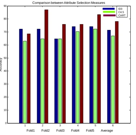
D. Comparison between Attribute Selection Measures
We have implemented the ID3, C4.5 CART algorithm and tested them on our experimental dataset. The results are shown on Table-II and Fig-4.
TABLEIII
1 2 3 4 5 6 0
10 20 30 40 50 60 70 80
90 Comparison between Attribute Selection Measures
Fold1 Fold2 Fold3 Fold4 Fold5 Average
A
ccu
ra
cy
ID3 C4.5 CART
Fig. 4 Comparison between attribute selection measures which shows the accuracy of each algorithms
From our results we observed that among the attribute selection measures C4.5 performs better than the ID3 algorithm, but CART performs even better both in respect of accuracy and time complexity.
In a previous research [11], the authors used the ID3 algorithm of decision tree induction methods and the average accuracy of this research was 71.481%. We have done this research and we have found 78.184% accuracy with the CART algorithm which is greater than previous research.
VII. CONCLUSION
In our research we choose three attribute selection measure algorithms to have a comparative study among them. As experimental data we have used the biomedical heart disease dataset. To classify dataset, we have implemented three different algorithms. Among these algorithms, CART
algorithm always generates a binary decision tree. That means the decision tree generated by CART algorithm has exactly two or no child. But the decision tree which is generated by other two algorithms may have two or more child.
Also, in respect of accuracy and time complexity CART algorithm performs better than the other two algorithms.
REFERENCES
[1] Jiawei Han and Micheline Kamber, “Data Mining Concepts and techniques”, 2nd ed., Morgan Kaufmann Publishers, San Francisco,
CA, 2007.
[2] Margaret H. Dunham, “Data Mining Introductory and Advanced Topics”, Published by Pearson Education (Singapur) Pte. Ltd. Delhi, India, 2004.
[3] D. E. Johnson, F. J. Oles, T. Zhang and T. Geotz, “ A Decision Tree Based Symbolic Rule Induction System for Text Categorization”, IBM Systems Journal, Vol. 41, No 3, 2002
[4] A. Juozapavicius and V. Rapsevicius, “Clustering through Decision Tree Construction in Geology”, Nonlinear Analysis: Modeling and Control, 2001, vol. 6, No 2, 29-41.
[5] Ahmed Sultan Al-Hegami, “Classical and Incremental Classification in Data Mining Process”, IJCSNS International Journal of Computer Science and Network Security, VOL.7 No.12, December 2007 . [6] Kusrini, Sri Hartati, ”Implementation of C4.5 algorithm to evaluate the
cancellation possibility of new student applicants at stmik amikom yogyakarta.”Proceedings of the International Conference on Electrical Engineering and Informatics Institut Teknologi Bandung, Indonesia June 17-19, 2007.
[7] Jason R. Beck, Maria E. Garcia, Mingyu Zhong, Michael Georgiopoulos, Georgios Anagnostopoulos “A Backward Adjusting Strategy for the C4.5 Decision Tree Classifier”, Beck, et al. 2007. [8] Quinlan, J. R., “C4.5: Programs for Machine Learning”, San Mateo,
CA: Morgan Kaufmann Publications, 1993.
[9] Quinlan, J. R., “Induction of Decision Trees”, Machine Learning, 1:1, Boston: Kluwer, Academic Publishers, 1986, 81-106.
[10] Rajeev Rastogi, Kyuseok Shim, “PUBLIC: A Decision Tree Classifier that Integrates Building and Pruning”Bell Laboratories.