A Biologically-Based Controlled Growth and Differentiation Model Using Delay Differential Equations: Development, Applications and Stability Analysis.

(1)

ABSTRACT

WHITAKER, SHREE YVONNE. A Biologically-Based Controlled Growth and Differentiation Model Using Delay Differential Equations: Development, Applications and Stability Analysis. (Under the direction of Hien T. Tran.)

(2)

(3)

(4)

Biography

(5)

Acknowledgments

“I am because we are.”

(6)

mentoring, opportunities and encouragement during my matriculation. To each of you, “Thank you”.

The very first signs of encouragement to pursue a Ph.D. in mathematics came from my Clark Atlanta University family. The chair of the mathematics department, Dr. A. A. Shabazz, empowered so many with his unique mix of pride and mathematics. My advisor at CAU, Dr. J. E. Wilkins, Jr. taught me to be meticulous and precise not only in mathematics, but in everything! Dr. Melvin Webb, the late Dr. Henry McBay and the staff of the ONR PRISM-D program set a solid foundation for me. They continuously insisted on nothing less than success. I am eternally grateful that these mentors recognized and nurtured my skills as a mathematician. To all of you, “Thank you”.

I am thankful for my family and friends who have followed my academic career and have always been encouraging. My parents and my sisters, Star, Andrea and Shelease, have always offered unconditional love and support. Their presence has been a safe haven for me as I weathered many storms. My best friend, Michael P. Taylor, has played an integral part in the success of attaining my Ph.D. His unrelenting faith in my abilities has been a foundation for my self-confidence. I am thankful that he was placed in my life during what has been, so far, one my greatest life challenges. Although it is an understatement, nevertheless I say “Thank you”.

(7)

List of Tables

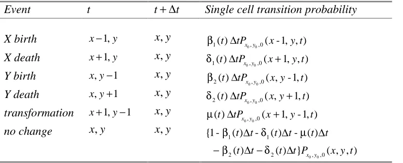
Table 1: Single Cell Event Probabilities in Time [ ,t t+ ∆t) for the Leroux et al. Model

...14

Table 2: Single Cell Event Probabilities in Time [t, t+∆t ) for the CGD Model...21

Table 3: Parameters Used to Predict Similar Results Among the Two Models ...30

Table 4: Parameters Used and Estimates Obtained Among the Two Models ...31

Table 5: First parameter set used in CGD model for spermatocytogenesis. ...51

Table 6: Second parameter set used in CGD model for spermatocytogenesis. ...53

Table 7: Developmental rates used in CGD model for hormesis (d=dose)...62

Table 8: Developmental rates used in CGD model for hormesis (d=dose)...64

(9)

List of Figures

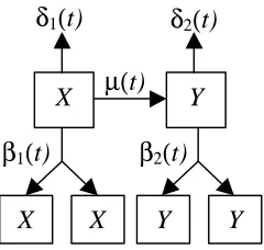
Figure 1: Developmental process of a tissue or organ as described by Leroux et al ...12

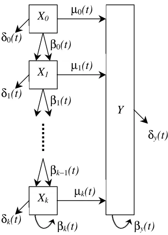
Figure 2: A general CGD system with k+2 states...18

Figure 3: Basic CGD model that predicts similar expectations and variances as the Leroux et al. model at time t=5...28

Figure 4: Modified CGD model that predicts results different from the Leroux et al. model. ...30

Figure 5: Expected number of type-Y cells as predicted by the Leroux et al. model and the CGD model using parameters in Table 4. ...32

Figure 6: Expected number of type-X cells as predicted by the Leroux et al. model and the CGD model using parameters in Table 4. ...33

Figure 7: The physical relationship of the Sertolli cell and developing cells...38

Figure 8: A schematic diagram of spermatogenesis ...42

Figure 9: Schematic diagram of CGD model for spermatocytogenesis...44

Figure 10: Cell Cycle with respect to time. ...45

Figure 11: Chaotic response for spermatocytogenesis using the CGD model.. ...52

Figure 12: Smooth response for spermatocytogenesis using CGD model ...54

Figure 13: Total number of cells using spermatocytogenesis CGD model...55

Figure 14: Schematic diagram of spermatocytogenesis CGD model for hormesis ...60

Figure 15: Dose-response relationship for spermatocytogenesis CGD model with a dose-dependent birth rate. ...62

(10)

Chapter 1: Background and Overview

The biological process of a developing tissue or organ in mammals is a complex activity. Systems of cells behave in various ways to reach the goal of forming a properly functioning tissue or organ. For normal development of a mammalian tissue or organ, the cell population must be within a specified interval at a critical time of development. A small deviation in the developmental process can result in malformation. The probability of malformation surfaces either when there are not enough cells produced to carry out a specific function or when a certain population of cells over-produces. The controlled growth and differentiation (CGD) model is intended to be able to predict the probability of malformation for a tissue or organ. The proposed model is based on the mathematical model developed by Leroux et al.; however, the CGD model has been designed to be more versatile, adaptable and thus more powerful than the original model. Due to its structure, the CGD model can also be used to explore intermediate stages of normal or abnormal development.

(11)

the use of delay differential equations in modeling. The chapter is concluded with a statement of the problem and an outline of the dissertation in Section 1.4.

1.1 Mathematical Modeling

Mathematical modeling has been used as a tool to understand various dynamical processes for centuries. However, the marriage of computer technology and mathematical modeling has recently allowed researchers to investigate problems that were once described as impossible and frivolous tasks. The ability to study system dynamics with elegance, speed and accuracy has been a great benefit for the advancement of scientific research.

While mathematics is unboubtingly a powerful tool, its power must be handled with great care and the highest respect when modeling. To use models properly requires not only an understanding of mathematics, but also a fundamental knowledge of the dynamic process under study. Once a mathematical model is developed for a particular system, this does not constitute the end of the problem. In fact, modeling can be thought of as an iterative process. After a model is constructed, it must be tested (preferably against real experimental data) for validity. This step is followed by continuous refinement until the mathematical model mimics the dynamical process as accurately as computationally possible.

(12)

and often involves several highly coupled dynamics all happening at once. Thus when building a mathematical model, the investigator must be careful not to construct a model that can not be understood at each intermediate step. To this end, assumptions in the development of a model may be physical, biological or purely mathematical [1]. It is quite common for researchers to impose restrictions on the model that compromises the true dynamics of the process. Otherwise, the model will be intractable and no further insight into the phenomena under scrutiny will be gained.

1.2 Biological Modeling

(13)

There has been considerable research into the mechanistic basis through which environmental exposures can initiate and promote disease processes. Much of this research has focused on the molecular and biochemical basis describing the interaction of chemical and physical agents with healthy tissue. Most environmental health risk assessments are focused on the rates of morbidity and mortality in human populations following an environmental exposure. The linkage between basic biology and disease incidence in environmental health is best described using a tool which is focused on the incidence of disease and which can fully utilize the emerging science [2, 3]. Disease incidence is generally described by counting events (e.g. disease prevalence in a population) or by early, functional failure of an entire organ system (e.g. disease incidence per year). Data endpoints such as these require a different mathematical treatment than the mathematical treatment applied to absorption, distribution and metabolism data endpoints [4]. While the mechanistic basis for understanding environmentally induced disease has progressed rapidly, biologically based mechanistic models of morbidity and mortality lag far behind. This gap in development is partially due to the difficulties in the mathematical treatment of these endpoints and partially due to gaps in scientists’ understanding of how the processes occur.

(14)

for cancer risk assessment. From the statistical point of view, this model provides a broad class of hazard functions for the analysis of data. Armitage and Doll [6] extended this model to use deterministic birth and death processes on the intermediate state in a two-stage model. Other researchers [7-23] have also contributed significant progress to this field. The models developed use biologically-based information and basic stochastic processes (generally interconnected birth-death processes with immigration and emigration) to reproduce the behavior of cells as they progress through the stages of cancer. Cancer is viewed as a multi-step process in which cells move from a controlled and systematic state of growth into a state of uncontrollable and chaotic growth [24, 25]. The basic assumption – that cancer is a disease of single cells rather than entire organ systems - on which these models were predicated, makes the mathematical modeling of carcinogenesis feasible.

(15)

form of the equations. Leroux et al. [36] developed the first biologically-based, stochastic model of developmental toxicity based on an interconnected birth-death process and using the first and second moments for the number of cells in a second stage of the model as an indicator of the probability of toxicity. The general view of development as modeled by Leroux et al. is a straightforward approach. However, the authors’ use of an uncontrolled, birth-death process for cellular growth is both biologically unreasonable (for small numbers of cells) and mathematically uncontrollable allowing for no clear numerical constraints on the size of the resulting organ. This issue will be addressed in a subsequent chapter of the dissertation.

1.3 Delay Differential Equations

The theory of differential equations allows investigators to study various phenomena. But differential equations only take into account the present state of the system. A system where the behavior includes information on former states of the system may force the model closer to reality. These types of systems are commonly called time-delay (time-lag) systems, delay differential equations or functional differential equations. So many natural processes in biology, medicine, chemistry, [37, 38] physics, etc. involve time delays that to ignore them is to ignore reality [39].

(16)

realistic model, it is also possible that the delay may induce instability or bad performance into closed-loop schemes [37, 38, 41, 42].

Incorporating time delays into a mathematical model can be a challenge. One issue to consider is the location of the time delay. The critical placement of the delay can yield results that are consistent with the observations or they can lead to very undesirable results. The type of delay incorporated into the system is also very important. Various authors have done extensive work on systems of single delays (see e.g. [43-47]). Another type of delay is a commensurate delay. These are delays where there exists a delays value, τ , such that all delays , (τ_i i=1,K, )n are rational multiples of τ . It is noted that there are some similarities between the commensurate and the single delay case [40]. Multiple delays involve more computations, but the results provide great insight into complicated systems. A mathematical model may incorporate constant time delays or delays that vary with time. The delay can be discrete or continuous. Depending upon the dynamics of the problem to be modeled, a system can be classified as a system of linear functional differential equation or a system of nonlinear functional differential equations.

(17)

lags from the system under study. For systems that have several delays, investigators have considered the problem of mixed delay-independent/delay-dependent stability [40].

1.4 Statement of Problem and Outline

The development of a biologically-based controlled growth and differentiation (CGD) model was inspired by the work of Leroux, Leisenring, Moolgavkar and Fautsman [36]. The original model was developed to address the shortcomings of methods currently used to evaluate the risk of developmental defects in humans as a result of exposure to potential toxic agents. Leroux et al. developed a mathematical model to describe aspects of the dynamic process of organogenesis, based on branching process models of cell kinetics. The work described in this dissertation presents an extension of the model by Leroux et al. [48]. The extended model allows the modeler a greater sense of control in the birth, death and migration of the cellular system at various stages. The CGD model retains the capabilities of the Leroux et al model while adding a higher level of versatility in the model by generalizing the system of ordinary differential equations that describe the developmental process.

(18)

of a true stem cell population. The biological phenomenon of tissue or organ development is formulated into a mathematical model by making biological assumptions. As stated previously, the Leroux et al. model assumes that there are two basic cell types: uncommitted cells (type-X) and committed cells (type-Y). To allow for mathematical tractability, the Leroux et al. model assumes that cells act independently of one another. The authors also assume that for each cell in the system, only one event (e.g. birth, death, and migration) can take place during a small time interval. The model dictates that cell replications result in daughter cells of the same cell type. Once a cell has become devoted to a particular phenotype, it is assumed that transformation back to the uncommitted stage does not occur. All of the aforementioned assumptions are incorporated into the development of the CGD model except one. While the CGD model does include the two distinct cell types (type-X and type-Y), the model is developed so that the type-X cell population passes through various stages of maturation before differentiation occurs. This modification greatly increases the versatility of the model.

(19)

(20)

Chapter 2: Model Development

This chapter is a detailed exposition of the development for the Leroux et al. model and the CGD model. Section 2.1 describes the re-derivation of the Leroux et al. model. Using the forward Kolmogorov, this straight forward approach is then extended to derive the CGD model in Section 2.2. The models are compared in Section 2.3 and the advantages of the CGD model are highlighted.

2.1 Leroux et al. Model

Equation Section 2

(21)

Figure 1: Developmental process of a tissue or organ as described by Leroux et al. The developmental parameters are birth (β_i( )t for i=1,2), death (δ_i( )t for i=1,2) and

transformation ( ( )µ t ).

In this model, the basic developmental process is divided into two main subpopulations. Type-X cells represent cells before commitment to differentiation whereas type-Y cells represent cells that have undergone a transformation and are committed to a phenotype. In addition, the following specific assumptions were made for the mathematical development of the model:

(i) cells act independently of one another;

(ii) the probability of more than one event occurring in a single cell in any small time interval ∆t is proportional to (o ∆t);

(iii) transformation is an irreversible process;

(iv) a cell in a particular population can only replicate to produce cells of the same population; and

(v) a malformation results when the number of committed cells ( ( )Y t ) is less than a critical number (Yc) at a specified time, tc (i.e., ( )Y tc <Yc).

µ(t)

β2(t)

β1(t)

X X Y Y

X Y

(22)

The type-X cell has the option to replicate, die or transform while the type-Y cell may either replicate or die. It is noted that the result of a cell replicating is two daughter cells that are a part of the original population (i.e., the daughter cells are members of the same population as the parent cell). The result of a cell dying is either removal of the cell from the population of properly functioning cells or actual death of a cell. A transformation is the result of a type-X cell moving from the population of uncommitted cells to the population of cells committed to differentiation.

The developmental rates for the system are denoted by β₁( )t (birth rate in X population), δ₁( )t (death rate in X population), β₂( )t (birth rate in Y population), δ₂( )t (death rate in Y population) and ( )µ t (transformation rate from X population to Y population). The meaning of the rate β₁( )t , for example, is that for the time interval [ , ) t t+ ∆t where ∆t is small, the probability of replication for a type- X cell is

1( )t t o( t)

β ∆ + ∆ where

0

( )

lim 0.

t

o t t

∆ → ∆∆ = (2.1)

The forward Kolmogorov equation for the transition probability can be expressed generally as

, , ( , , ) Pr[ ( ) , ( ) | ( ) , ( ) ].

x y t X t t x Y t t y X t x Y t y

P_{% %} x y t+ ∆t = + ∆ = + ∆ = = % = % (2.2) Since only certain events, which are summarized in Table 1, can occur in a small time interval t∆ , the transition probability

0, 0,0

x y

(23)

0 0 0 0

0 0

, ,0 1 , ,0

1 , ,0

, ,0

2 , ,0

1 1

( , , ) ( 1) ( ) ( 1, , ) ( 1) ( ) ( 1, , )

( 1) ( ) ( 1, 1, )

( 1) ( ) ( , 1, ) ( 1) ( ) ( , 1, )

[1 ( ) ( ) ( )

x y x y

P x y t t x t tP x y t

x t tP x y t

x t tP x y t

y t tP x y t

x t t x t t x t t y β δ µ β δ β δ µ + ∆ = − ∆ − + + ∆ + + + ∆ + − + − ∆ − + + ∆ + + − ∆ − ∆ − ∆ − 0 0

2( )t t y 2( )t t P] x y, ,0( , , ).x y t

β ∆ − δ ∆

(2.3)

Table 1: Single Cell Event Probabilities in Time [ ,t t+ ∆t) for the Leroux et al. Model Event t t+ ∆t Single cell transition probability

X birth x−1,y x y,

0 0

1( )t tPx,y,0( -1, , )x y t

β ∆

X death x+1,y x y,

0 0

1( )t tPx,y,0(x 1, , )y t

δ ∆ +

Y birth x y, −1 x y,

0 0

2( )t tPx,y,0( ,x y-1, )t

β ∆

Y death x y, +1 x y,

0 0

2( )t tPx,y,0( ,x y 1, )t

δ ∆ +

transformation x+1,y−1 x y,

0, 0,0

( )t tPx y (x 1,y- 1, )t

µ ∆ +

no change x y, x y,

0 0

1 1

2 2 , ,0

{1 - ( ) - ( ) - ( )

( ) ( ) } _x _y ( , , )

t t t t t t

t t t t P x y t

β δ µ

β δ

∆ ∆ ∆

− ∆ − ∆

Recall that for discrete random variables X and Y, the moment generating function for a time interval of length ∆t given the initial values x0 and y0 is given by

0 0

0 0 , ,0

[ ( ) ( ) | (0) , (0) ] ( , , ).

y

n p n p

x y x

E X t+ ∆t Y t+ ∆t X =x Y = y =

∑

x y P x y t+ ∆t (2.4)

Hence, using equations (2.3) and (2.4) the first moment (mean) for X is defined as

0

1 0

0

(0) , (0) ]

[ ( ) ( ) |

[ ( ) |

X x Y y

E X t t Y t t E X t t

= =

= = =

+ ∆ + ∆

(24)

0, 0,0( , , ) y

x y x

xP x y t t

=

∑

+ ∆ (2.6)

0 0 0 0

0 0

0 0 0 0

1 , ,0 1 , ,0

, ,0

2 , ,0 2 , ,0

1 1 2

[ ( 1) ( ) ( 1, , ) ( 1, , )

( 1, 1, )

( , 1, ) ( , 1, )

[1 ( ) ( ) ( ) ( )

( 1) ( ) ( 1) ( )

y

x y x y

x

x y

x y x y

x x t tP x y t x y t

x y t

x y t x y t

x x t t x t t x t t y t t

x x t tP x x t tP

x y t tP x y t tP

β β δ µ β δ µ β δ − ∆ − + + + + − + − + + + − ∆ − ∆ − ∆ − ∆ = + ∆ + ∆ − ∆ + ∆

∑

0 0

2( ) ] x y, ,0( , , ).

yδ t t P x y t

− ∆

(2.7)

The first term in equation (2.7) can be simplified by rescaling the summation indices as follows:

0 0 0 0

1 , ,0 1 , ,0

( 1) ( ) ( 1, , ) ( 1) ( ) ( , , )

y y

x y x y

x x

x x β t tP x y t x xβ t tP x y t

′

′ ′ ′

− ∆ − = + ∆

∑

(2.8)

0 0 0 0

1 1

2

, ,0 , ,0

( ) ( , , ) ( ) ( , , )

y y

x y x y

x x

x β t tP x y t xβ t tP x y t

′ ′

′ ′ ′ ′

=

∑

∆ +

∑

∆ (2.9)

2

1 1

[ ( )] ( ) [ ( )] ( ) , E X t β t t E X t β t t

= ∆ + ∆ (2.10)

where 2

[ ( )]

E X t is used to denote 2

0 0

[ ( ) | (0) , (0) ]

E X t X =x Y = y . Proceeding in a similar manner for the remaining terms in equation (2.7) leads to

{

1 1

}

[ ( )] ( ) ( ) ( ) 1 [ ( )].

E X t+ ∆ =t β t ∆ −t δ t ∆ −t µ t ∆ +t E X t (2.11) Subtracting [ ( )]E X t from both sides of equation (2.11) and then dividing both sides by

t

∆ yields

{

1 1

}

[ ( )] [ ( )]

( ) ( ) ( ) [ ( )], E X t t E X t

t t t E X t

t β δ µ

+ ∆ − ₌ ₋ ₋

∆ (2.12)

which, in the limit as ∆tgoes to zero, gives

{

1 1

}

[ ( )] ( ) ( ) ( ) [ ( )]. d

E X t t t t E X t

(25)

The expected value (mean) for the random variable Y can be derived in a similar manner. The variances and the covariance (i.e., E X[ 2( ) |t X(0)= x Y₀, (0)= y₀] ,

2

0 0

[ ( ) | (0) , (0) ]

E Y t X =x Y = y and E X t Y t[ ( ) ( ) | (0)X =x Y0, (0)= y0], respectively)

are also calculated by following the same procedure. Therefore, the system of ordinary differential equations describing the means, variances and covariance for the number of cells in states X and Y at any time t is given by

{

1 1

}

[ ( )] ( ) ( ) ( ) [ ( )] d

dt = β −δ −µ (2.14)

{

2 2

}

[ ( )] ( ) ( ) [ ( )] ( ) [ ( )] d

E Y t t t E Y t t E X t

dt = β −δ +µ (2.15)

{

}

{

}

2 2

1 1

[ ( )] 2 ( ) ( ) ( ) [ ( )] ( ) ( ) ( ) [ ( )] d

E X t t t t E X t

dt

t t t E X t

β δ µ β δ µ = − − + + + (2.16)

{

}

{

}

2 2

2 2 2 2

[ ( )] 2 ( ) ( ) [ ( )] ( ) ( ) [ ( )] ( ) [ ( )] 2 ( ) [ ( ) ( )]

d

E Y t t t E Y t t t E Y t

dt

t E X t t E X t Y t

β δ β δ

µ µ

= − + +

+ +

(2.17)

{

1 1 2 2

}

2

[ ( ) ( )] ( ) ( ) ( ) ( ) ( ) [ ( ) ( )] ( ) [ ( )] ( ) [ ( )].

d

E X t Y t t t t t t E X t Y t

dt

t E X t t E X t

β δ β δ µ

µ µ

= − + − −

− +

(2.18)

The above mathematical model is identical to the one derived by Leroux et al. in which the authors considered a partial differential equation for the generating function for

( )

X t and ( )Y t . Particularly, Leroux et al. chose the generating function for X t( ) and ( )

Y t to be

(26)

Using the Kolmogorov forward equations, Leroux et al. derived the following partial differential equation for the generating function:

1

1 1

1

2 2

( , , ) ( , , )[( 1) ( ) ( 1) ( ) ( 1) ( )]

( , , )[( 1) ( ) ( 1) ( )]. u v t u u v t u t

t u

u t u v v t

v u v t v t v t

v ϕ ϕ λ µ ϕ λ µ − − − ∂ ₌ ∂ ₋ ∂ ∂ + − + − ∂ + − + − ∂ (2.20)

In the case of constant rates, the system of differential equations (2.14)-(2.18) is a linear system of ordinary differential equations with a constant coefficient matrix of the form

( ) ( )

y tr′ =Ay tr (2.21)

where y tr( )=( [ ( )], [ ( )], [E X t E Y t E X2( )], [t E Y2( )], [ ( ) ( )])t E X t Y t T and

1 1

2 2

1 1 1 1

2 2 2 2

1 1 2 2

0 0 0 0

0 0 0

.

0 2( ) 0 0

0 2( ) 2

0 0 A β δ µ µ β δ β δ µ β δ µ µ β δ β δ µ µ µ β δ µ β δ − −    ₋      = + + − −  ₊ ₋     ₋ _{− − +} ₋    (2.22)

The exact solution can be written in terms of the eigenvalues and eigenvectors of the matrix A (see e.g., [49]).

2.2 Controlled Growth and Differentiation Model

(27)

expand their model to larger, more detailed biological systems with intermediate stages. To this end, attention is focused on modifications of the Leroux et al. model that put greater emphasis on the control of growth and differentiation. The CGD model assumes that daughter cells advance to the next stage of development while the Leroux et al. model assumes that the daughter cells rejoin the original population of the parent cells. This assumption of a linear birth-death process in both the type-X and type-Y of the Leroux et al. model is not adopted in the CGD model. More specifically, a multistate developmental process with separate growth phases in the type-X cells and a linear birth-death process on the type-Y cells are considered. A schematic diagram of the CGD model is illustrated in Figure 2.

Figure 2: A general CGD system with k+2 states. This system allows the cells to go through various levels of maturation before committing to the differentiation process.

βy(t)

δy(t)

Y β1(t)

β0(t)

µ0(t)

X0

δ0(t)

µ1(t) X1

δ1(t)

βk−1(t)

βk(t)

Xk

δk(t)

(28)

In this system, there are k+1 specific type-X populations denoted as type-X_i, where 0,1, 2, ,

i= K k. Each of the type-X cell populations represents cells prior to commitment to differentiation. Moreover, as a cell moves from one stage, for example from X_i, to the next stage, Xi+1, it matures in the developmental process. By setting

0 i

µ = , for one or more values of i, greater control is allowed in the type-X cells prior to differentiation. Eventually, the uncommitted cell will undergo a change and join the population of cells already committed to performing a specific function of a tissue or organ. This process by which an uncommitted cell becomes a cell committed to differentiation is termed transformation. Type-Y cells denote the population of cells committed to differentiation. If the first moments in the CGD model are represented by n random variables, then there are n first moments, n second (squared) moments, and

( 1) 2

n n−

second (cross product) moments. The following equation can be used to determine the dimension of the CGD model when the number of random variables is specified

( 1)

2 .

2 CGD

n n

E = n+ − (2.23)

The assumptions and the parameters in the model have the same basic definition as those in the Leroux et al. model (see Section 2.1). More specifically, for each

type-i

X cell, one of three outcomes is possible: division of the cell into two type-Xi+1

(29)

one of two outcomes: division into two type-Y daughter cells or death prior to division. In the type-Y population death is understood to include actual death of a cell or removal from the pool of fully committed cells contributing to the development and function of the tissue or organ in consideration.

The developmental rates are again denoted by β_i( )t (birth rate in a X_ipopulation), ( )

i t

δ (death rate in a X_ipopulation), β_y( )t (birth rate in the Y population), δ_y( )t (death

(30)

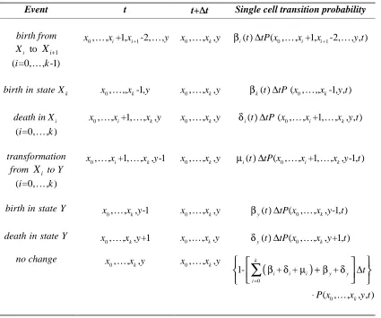
Table 2:Single Cell Event Probabilities in Time [ ,t t+ ∆t) for the CGD Model

Event t t+∆∆t Single cell transition probability

birth from

i

X to X_i₊₁ ( =0,i K, -1)k

0, , +1,i i+1-2, ,

x Kx x Ky x₀,K, ,x y_k β_i(t) ∆tP x( ,₀ K, +1,x_i x_i₊₁-2,K, , )y t

k

birth in state X x0,K,,xk-1,y x0,K, ,x yk βk(t) ∆tP x( ,0 K,, -1, , )xk y t

death inXi

( =0,i K, )k

0, , +1,i , ,k

x Kx Kx y x0,K, ,x yk δi(t) ∆tP x( ,0 K, +1,xi K, , , )x y tk

transformation from X_i to Y

( =0,i K, )k

0, , +1,i , , -1k

x Kx Kx y x₀,K, ,x y_k µ_i(t) ∆tP x( ,₀ K, +1,x_i K, , -1, )x y_k t

birth in state Y

0, , , -1k

x Kx y x₀,K, ,x y_k β_y(t) ∆tP x( ,₀ K, , -1, ) x y_k t

death in state Y

0, , , +1k

x Kx y x0,K, ,x yk δy(t) ∆tP x( ,0 K, , +1, )x yk t

no change

0, , ,k

x Kx y x₀,K, ,x y_k

(

)

0

1- + + +

( , , , , )

k

i i i y y

i

k

t P x x y t

β δ µ β δ

=

+ ∆

⋅

   

 _ _ 

 



∑



K

(31)

00 0 0

, , , ,0 0

1

, , , ,0 0 1

0

, , , ,0 0

0

( , , , , )

( 1) ( ) ( , , 1, 2, , , , )

( 1) ( ) ( , , 1, , )

( 1) ( ) ( , , 1, , , , )

( 1)

k

x x y k

k

i i x x y i i k

i

k k x x y k

k

i i x x y i k

i i

P x x y t t

x t tP x x x x y t

x t tP x x y t

x t tP x x x y t

x β β δ µ − + = = +∆ = + ∆ + − + − ∆ − + + ∆ + + +

∑

K K K K K K K K K K

00 0 0

00 0

, , , ,0 0

0

, , , ,0 0

, , ,

0

( ) ( , , 1, , , 1, )

( 1) ( ) ( , , , 1, )

1 ( ( ) ( ) ( )) ( ( ) ( ))

k

k k

k

i x x y i k

i

y x x y k

k

i i i i y y x x y

i

t tP x x x y t

y t tP x x y t

x t t t t y t t t P

β δ β δ µ β δ = = ∆ + − + − ∆ − + + ∆ +   + −_ + + ∆ − + ∆_  

∑

K K K K K K K K

0,0( ,x0 K,x y tk, , ).

(2.24)

Since an objective of the CGD model is to estimate the average number of cells that accumulate in stage Y at a particular time of the developmental process, the expected value (first moment) for each random variable is calculated. This is done in the same manner as for the re-derivation the Leroux et al. model in Section 2.1.

For an arbitrary discrete random variable Xj and a discrete random variable Y, the moments for a time interval of length ∆t given the initial values

00, ,10 , k-1,0, k0 and 0

x x K x x y is defined to be

(

)

00 0 0

0 1

0 0

1

, , , ,0 0 .

( ) | (0) , (0)

( , , , , , )

k k

n p

j j j

n p

j x x y k

x x x y

y

E X t t Y t t X x Y y

x P x x x y t t

 

 + ∆ + ∆ = = 

=

∑∑ ∑∑

K _K K + ∆ (2.25)

(32)

{

}

1 1

[ j( )] j( ) j( ) j( ) [ j( )] 2 j ( ) [ j ( )]. d

E X t t t t E X t t E X t

dt = − β +δ +µ + β − − (2.26)

Detailed calculations of the expected value of X_j, for j=0,1,K,k−1 is provided below. The following process can be repeated to obtain the remaining first and second moments. Based on equation (2.4) the expected value for the random variable Xj can be written as

(

)

0 1 1 0 1 0 1

1 1 0 1

0 1

0

( 1) ( ) ( , , 1, 2, , , , )

( 1) ( ) ( , , 1, 2, , , , ) ( 1) ( ) ( , ,

{

k

j

k

j i i i i k

x x x y i

i j i j

j j j j j k

j k k k

E X t t

x x t tP x x x x y t

x x t tP x x x x y t

x x t tP x x

β β β β − + = ≠ − ≠ − − − +  + ∆    = + ∆ + − + + ∆ + − + + ∆ + − + − ∆

∑∑ ∑∑ ∑

K K K

K K K K K 0 0 1

1 1 0 1

0

0 0

1

1, , )

( 1) ( ) ( , , 1, , , , )

( 1) ( ) ( , , 1, , , , ) ( 1) ( ) ( , , 1, , , 1, )

( 1)

k

j i i i k

i i j i j

j j j j k

k

j i i i k

i i j i j j j

y t

x x t tP x x x y t

x x t tP x x x y t

x x t tP x x x y t

x x δ δ δ µ = ≠ − ≠ − − − = ≠ − ≠ − − + + ∆ + + + ∆ + + + ∆ + + + ∆ + − + +

∑

K K K K K K K K

1 0 1

0

0 0

( ) ( , , 1, , , 1, ) ( 1) ( ) ( , , 1, , , 1, )

( 1) ( ) ( , , , 1, ) ( 1) ( , , , 1, )

1 ( ( ) ( ) ( )) ( ( ) ( )) ( , , , ,

j j k

j j j j k

j y k j y k

k

j i i i i y y k

i

t tP x x x y t

x x t tP x x x y t

x y t tP x x y t x y tP x x y t

x x t t t t y t t t P x x y

µ µ β δ β δ µ β δ − − = ∆ + − + + ∆ + − + − ∆ − + + ∆ +   + _ − + + ∆ − + ∆ _ 

∑

 K K K K K K

K t) .

}

(33)

At this point all the probability density functions are rescaled. Also denote

0

( , , k, , )

P x … x y t simply by

( , , ).

P x y tv (2.28)

Thus, equation (2.27) becomes

(

)

1

0 1 1 1 1 1 0 1 ( ) ( , , )

( 2) ( ) ( , , )

( 1) ( ) ( , , ) ( ) ( , , ) ( ) ( , , ) ( ) ( , , )

( 1) (

{

k

j j i i

x y i

i j i j

j j j

j j j j k k

k

j i i j j j

i i j i j

j j j

E X t t x x t tP x y t

x x t tP x y t

x x t tP x y t x x t tP x y t x x t tP x y t x x t tP x y t

x x t

β β β β δ δ δ − = ≠ − ≠ − − − − = ≠ − ≠  + ∆ = ∆   + + ∆ + − ∆ + ∆ + ∆ + ∆ + −

∑∑ ∑

∑

v v v v v v v 1 1 0 1 0 ) ( , , ) ( ) ( , , ) ( ) ( , , )

( 1) ( ) ( , , )

( ) ( , , ) ( ) ( , , )

( , , ) ( ( ) ( ) ( )) ( , , ) ( ( )

k

j i i j j j

i i j i j

j j j

j y j y

k

j j i i i i

i

j y

tP x y t

x x t tP x y t x x t tP x y t

x x t tP x y t

x y t tP x y t x y t tP x y t

x P x y t x x t t t tP x y t x y t

µ µ µ β δ β δ µ β δ − − = ≠ − ≠ = ∆ + ∆ + ∆ + − ∆ + ∆ + ∆ + − + + ∆ − +

∑

v v v v v v v v ( )) ( , , ) .

}

y t ∆tP x y tv

(2.29)

Further simplifications reduce to

1 1

[ ( )] {2 ( ) ( , , )

( ( ) ( ) ( )) ( , , ) ( , , )}.

j j j

x y

j j j j j

E X t t t t x P x y t

t t t t x P x y t x P x y t β

β δ µ

− −

+ ∆ = ∆

− + + ∆ +

∑∑

_v v

v v (2.30)

(34)

(

)

00 10 1,0 0 0

0 1

0 0

1

, , , , , ,0 0 .

( ) | (0) , (0)

( , , , , , )

k k

k

n p

j j j

n p

j x x x x y k

x x x y

y

E X t t Y t t X x Y y

x P x x x y t t −

 

 + ∆ + ∆ = = 

=

∑∑ ∑∑

K _K K + ∆ (2.31)

Thus with n=1 and p=0, equation (2.30) reduces to

1 1

[ ( )] 2 ( ) [ ( )]

( ( ) ( ) ( )) [ ( )] [ ( )].

j j j

j j j j j

E X t t t t E X t

t t t t E X t E X t β

β δ µ

− −

+ ∆ = ∆

− + + ∆ + (2.32)

Finally, subtracting [E X t_j( )] from both sides of equation (2.32), dividing by ∆t and letting ∆t approaches zero yields

0

1 1

[ ( )] [ ( )] lim

2 ( ) [ ( )] ( ( ) ( ) ( )) [ ( )],

j j

t

j j j j j j

E X t t E X t t

t E X t t t t E X t

β β δ µ ∆ → − − + ∆ −    _∆    = − + + (2.33) or equivalently 1 1

[ _j( )] 2 _j ( ) [ _j ( )] ( _j( ) _j( ) _j( )) [ _j( )]. d

E X t t E X t t t t E X t

dt = β − − − β +δ +µ (2.34)

The remaining first moments and the second moments for the discrete random variables are calculated in a similar manner. The result is the following system of ordinary differential equations with time dependent developmental rates (unless otherwise stated, j =0,1, 2,K,k−1):

{

}

1 1

[ _j( )] _j( ) _j( ) _j( ) [ _j( )] 2 _j ( ) [ _j ( )] d

dt = − β +δ +µ + β − − (2.35)

{

}

1 1

[ _k( )] _k( ) _k( ) _k( ) [ _k( )] 2 _k ( ) [ _k ( )] d

dt = β −δ −µ + β − − (2.36)

{

}

[ ( )] ( ) ( ) [ ( )] ( ) [ ( )] k

y y i i

d

E Y t t t E Y t t E X t

(35)

{

}

{

}

2 2

1 1 1 1

[ ( )] 2 ( ) ( ) ( ) [ ( )] ( ) ( ) ( ) [ ( )]

4 ( ) [ ( )] 4 ( ) [ ( ) ( )]

j j j j j

j j j j

j j j j j

d

dt

t t t E X t

t E X t t E X t X t

β δ µ β δ µ β ₋ ₋ β ₋ ₋ = − + + + + + + + (2.38)

{

}

{

}

2 2

1 1 1 1

[ ( )] 2 ( ) ( ) ( ) [ ( )] ( ) ( ) ( ) [ ( )]

4 ( ) [ ( )] 4 ( ) [ ( ) ( )]

k k k k k

k k k k

k k k k k

d

dt

t t t E X t

t E X t t E X t X t

β δ µ β δ µ β ₋ ₋ β ₋ ₋ = − − + + + + + (2.39)

{

}

{

}

2 2 0 0

[ ( )] 2 ( ) ( ) [ ( )] ( ) ( ) [ ( )]

[ ( )] 2 [ ( ) ( )]

y y

k k

i i i i

i i

d

E Y t t t E Y t

dt

t t E Y t

E X t E X t Y t

β δ β δ µ µ = = = − + + +

∑

+

∑

(2.40)

{

}

1 1 1 1

( ) ( ) ( ) ( ) ( ) ( )

[ ( ) ( )] [ ( ) ( )]

2 ( ) [ ( ) ( )] 2 ( ) [ ( ) ( )] where , 0,1, 2, , and , are not

consecutive integers

l l l j j j

l j l j

l l j j l j

t t t t t t

d

E X t X t E X t X t

dt

t E X t X t t E X t X t

l j k l j

l j β δ µ β δ µ β₋ ₋ β ₋ ₋ + + + + + = − + + = ≠ K (2.41)

{

}

2

1 1 1 1 1

2 2

1 1 1 1

[ ( ) ( )] 2 ( ) [ ( )] 2 ( ) [ ( )] 2 ( ) [ ( ) ( )]

( ) ( ) ( ) ( ) ( ) ( ) [ ( ) ( )]

j j j j j j

j j j

j j j j j j j j

d

E X t X t t E X t t E X t

dt

t E X t X t

t t t t t t E X t X t

β β β β δ µ β δ µ − − − − − − − − − − − = − + + − + + + + + (2.42)

{

}

2

1 1 1 1 1

2 2

1 1 1 1

[ ( ) ( )] 2 ( ) [ ( )] 2 ( ) [ ( )] 2 ( ) [ ( ) ( )]

( ) ( ) ( ) ( ) ( ) ( ) [ ( ) ( )]

k k k k k k

k k k

k k k k k k k k

d

E X t X t t E X t t E X t

dt

t E X t X t

t t t t t t E X t X t

(36)

{

}

1 1

0

[ ( ) ( )] ( ) ( ) ( ) ( ) ( ) [ ( ) ( )] 2 ( ) [ ( ) ( )] ( ) [ ( )]

( ) [ ( ) ( )]. for 0,1, 2, , 1

j y y j j j j

j j j j

k

i j i

i d

dt

t E X t Y t t E X t

t E X t X t j k

β δ β δ µ

β µ

µ

− −

=

= − − − −

+ −

+

∑

= _K −

(2.44)

{

}

1 1

0

[ ( ) ( )] ( ) ( ) ( ) ( ) ( ) [ ( ) ( )] 2 ( ) [ ( ) ( )] ( ) [ ( )]

( ) [ ( ) ( )].

k y y k k k k

k k k k

k

i k i

i d

dt

t E X t Y t t E X t t E X t X t

β δ β δ µ

β µ

µ

− −

=

= − + − −

+ −

+

∑

(2.45)

2.3 Comparison of Models

In this section, the Leroux et al. model and the CGD model are examined and compared in an effort to highlight the most useful and biologically realistic model for the developmental process as it relates to animals. For a description on the experimental aspects and how the in vitro data were used to estimate cell kinetic rates in both models see the Leroux et al. paper. In addition, all computations were done using computer codes written in the MATLAB/Simulink environment (The Math Works, Inc., Natick, Massachusetts).

(37)

by the Leroux et al. model. Specifically, consider the very simple developmental CGD model depicted in Figure 3.

Figure 3: Basic CGD model that predicts similar expectations and variances as the Leroux et al. model at time t=5. Table 3 lists all of the developmental rates associated

with this particular CGD model.

The system of ordinary differential equations describing the means, variances and covariances for the number of cells in states Xj (j=0,1) and Y is given below.

{

}

0 0 0 0 0

[ ( )] ( ) ( ) ( ) [ ( )] d

dt = − β +δ +µ (2.46)

{

}

1 1 1 1 1 0 0

[ ( )] ( ) ( ) ( ) [ ( )] 2 ( ) [ ( )] d

E X t t t t E X t t E X t

dt = β −δ −µ + β (2.47)

{

}

0 0 1 1

[ ( )] _y( ) _y( ) [ ( )] ( ) [ ( )] ( ) [ ( )] d

E Y t t t E Y t t E X t t E X t

dt = β −δ +µ +µ (2.48)

{

}

{

}

2 2

0 0 0 0 0

0 0 0 0

[ ( )] 2 ( ) ( ) ( ) [ ( )] ( ) ( ) ( ) [ ( )] d

dt

t t t E X t

β δ µ

= − + +

+ + +

(2.49) δy(t)

µ0(t)

µ1(t)

β1(t)

X1

β0(t)

δ1(t)

δ0(t)

βy(t)

(38)

{

}

{

}

2 2

1 1 1 1 1

1 1 1 1

0 0 0 0 1

[ ( )] 2 ( ) ( ) ( ) [ ( )]

( ) ( ) ( ) [ ( )]

4 ( ) [ ( )] 4 ( ) [ ( ) ( )] d

dt

t t t E X t

t E X t t E X t X t

β δ µ β δ µ β β = − − + + + + + (2.50)

{

}

{

}

{

}

2 2

0 0 1 1

[ ( )] 2 ( ) ( ) [ ( )] ( ) ( ) [ ( )] [ ( )] [ ( )]

2 [ ( ) ( )] [ ( ) ( )]

y y y y

d

E Y t t t E Y t t t E Y t

dt

E X t E X t

E X t Y t E X t Y t

β δ β δ µ µ µ µ = − + + + + + + (2.51)

{

}

2

0 1 0 0 0 0

1 1 1 0 0 0 0 1

[ ( ) ( )] 2 ( ) [ ( )] 2 ( ) [ ( )]

( ) ( ) ( ) ( ) ( ) ( ) [ ( ) ( )] d

E X t X t t E X t t E X t dt

t t t t t t E X t X t

β β β δ µ β δ µ = − + + − − − − − (2.52)

{

}

0 0 0 0 0

2

0 0 0 0 1 0 1

[ ( ) ( )] ( ) ( ) ( ) ( ) ( ) [ ( ) ( )]

( ) [ ( )] ( ) [ ( )] ( ) [ ( ) ( )]

y y

d

dt

t E X t t E X t t E X t X t

β δ β δ µ µ µ µ = − − − − − + + (2.53)

{

}

1 1 1 1 1

2

1 1 1 1

0 0 1 0 0

[ ( ) ( )] ( ) ( ) ( ) ( ) ( ) [ ( ) ( )] ( ) [ ( )] ( ) [ ( )]

( ) [ ( ) ( )] 2 [ ( ) ( )]

y y

d

dt

t E X t t E X t

t E X t X t E X t Y t

β δ β δ µ µ µ µ β = − + − − − + + + (2.54)

(39)

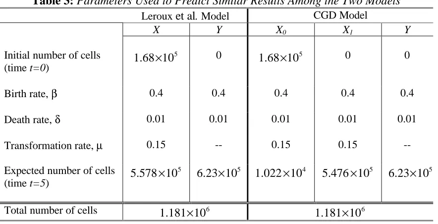
Table 3: Parameters Used to Predict Similar Results Among the Two Models

Leroux et al. Model CGD Model

X Y X0 X1 Y

Initial number of cells (time t=0)

5

1.68 10× 0 1.68 10× 5 0 0

Birth rate, β 0.4 0.4 0.4 0.4 0.4

Death rate, δ 0.01 0.01 0.01 0.01 0.01

Transformation rate, µ 0.15 -- 0.15 0.15

--Expected number of cells (time t=5)

5

5.578 10× 5

6.23 10× 4

1.022 10× 5

5.476 10× 5

6.23 10×

Total number of cells 6

1.181 10× 6

1.181 10×

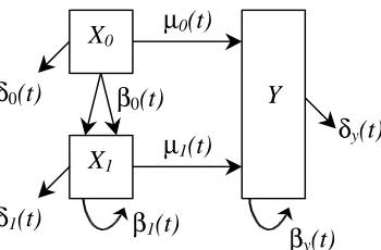
However, one major difference between the two models is the ability of the CGD model to deplete the population of X cells under constant rates while still maintaining the same distribution of Y cells. This can be illustrated using the simple CGD model in Figure 4.

Figure 4: Modified CGD model that predicts results different from the Leroux et al. model. Table 4 lists all of the developmental rates associated with this particular CGD

β0(t)

X0

δ0(t)

β1(t)

µ1(t)

δ1(t)

X1

δy(t)

βy(t)

(40)

The set of parameter values used to compare the two models is shown in Table 4.

Table 4: Parameters Used and Estimates Obtained Among the Two Models

Leroux et al. Model CGD Model

X Y X0 X1 Y

Initial number of cells (time t=0)

5

1.68 10× 0 5

1.68 10× 0 0

Birth rate, β 0.4 0.4 0.4 0.4 0.4

Death rate, δ 0.01 0.01 0.01 0.4 0.01

Transformation rate, µ 0.15 -- 0 0.5174

--Expected number of cells (time t=5)

5

5.58 10× 6.23 10× 5 2.16 10× 4 6.69 10× 4 6.23 10× 5

Total number of cells 6

1.181 10× 7.115 10× 5

As before, both the Leroux et al. model and the simple CGD model (Figure 4) start with the same initial conditions. The type-X (Leroux et al. model) and type-X0(CGD

model) subpopulations each consist of 1.68 10× 8cells at time t=0 while the remaining states start with a cell population of zero. In this example, the transformation rate for the X0 state is set equal to zero; thus, only cells from the X1 state migrate to the Y

(41)

increasing δ₁ and µ₁. Nevertheless, the results are quite different from those of the Leroux et al. model.

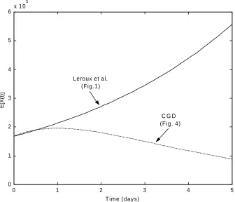
The expected value of type-Y cells for both models agree at time t=5, as seen in Figure 5, but differ slightly at other time points.

Figure 5: Expected number of type-Y cells as predicted by the Leroux et al. model and the CGD model using parameters in Table 4.

This implies that the CGD model can indeed be tailored to produce the same number of committed (type-Y) cells as the Leroux et al. model. However, Figure 6 reveals that the models produce different expected numbers of uncommitted (type-X) cells.

0 1 2 3 4 5

0 1 2 3 4 5 6 7x 1 0

5

Time (days)

E

[Y(t)]

Leroux et al. (Fig.1) C G D

(42)

Figure 6: Expected number of type-X cells as predicted by the Leroux et al. model and the CGD model using parameters in Table 4.

As seen from Table 4, both models start out with the same number of uncommitted cells and the birth rates in each type-X population are the same. However, due to the structure of the CGD model, the type-X1cells are able to have higher death and

transformation rates. Biologically, this means that all of the committed (type-Y) cells have type-X₁ precursor cells and that the population of uncommitted cells will eventually die out. This ultimately results in a stable population of committed cells at greater times, unlike the Leroux et al. model that will continue to grow.

0 1 2 3 4 5

0 1 2 3 4 5 6 x 1 0

5

Time (days)

E

[X(t)]

Leroux et al. (Fig.1)

(43)

Provided actual cell size is consistent throughout development, the expected final size of the tissue/organ is simply computed as the total number of cells present in the system at timet=5. The total number of cells, which is defined to be the sum of all expectations of type-X and type-Y cells, present in the Leroux et al. model exceeds the number of cells present in the CGD model. This implies that, for sufficiently large time, the size of the tissue/organ might become unrealistically large. It is also important to note that in order to reduce the number of committed cells in the Leroux et al. model, there are a few options available:

(i) reduce the initial number of type-X cells

(ii) reduce the birth rate of the type-X and/or type-Y cells (iii) increase the death rate of the type-X and/or type-Y cells (iv) use more complicated time-varying rates

In each case, the ability to accurately reflect the biological dynamics of the development process is compromised. If option (i) is pursued, the experimental data and the mathematical model may not agree initially. If option (ii) or (iii) is incorporated, the cellular kinetics of the system may not be modeled accurately. In any event, the end result is that the mathematical model does not realistically duplicate the biological dynamics of the system. Option (iv) requires significantly more knowledge of the time-varying nature of the developmental rates in the system.

(44)

(45)

Equation Section 3

Chapter 3: Controlled Growth and Differentiation Model

Applications

Biologically-based mathematical models are developed based on the observations recorded by scientists. The models are usually validated against experimental data (when available) and then used to predict the results of various dynamical processes. The information gained from a biological model can also be used to assist in the judicious design of laboratory experiments, thereby reducing the unnecessary loss of valuable time and resources. The ultimate objective of the CGD model is to provide a more biologically realistic model for describing the dynamic process of organogenesis. As a step toward this goal, this chapter explores two applications for the CGD model.

(46)

The second application is a demonstration of how the spermatocytogenesis model can be used to model hormesis. The developmental rates for the spermatocytogenesis CGD model are changed from constant rates to dose-dependent rates. Thus for a given time, a dose-response curve is generated for an agent that produces a hormetic effect.

3.1 Spermatogenesis

(47)

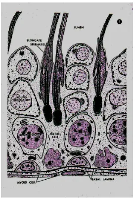
support roughly 15 to 20 cells. Figure 7 shows the relationship between the Sertolli cell and developing cells.

(48)

3.1.1 Cellular Dynamics

During germ cell development, there are three major phases: spermatocytogenesis, meiosis and spermiogenesis. Cells in the earliest stage of spermatogenesis are in the spermatocytogenesis phase and are referred to as spermatogonia. These immature germ cells originate from stem cells that have undergone asymmetric division: a process where a stem cell divides and produces another stem cell (to maintain the original stem cell population) and an immature specialized cell. In this case, the future specialized cells are spermatogonia. Spermatogonia reside primarily at the base of the seminiferous tubule. The immature germ cell attaches itself to the Sertoli cell, its source of nutrition. As the cell continues through the developmental process, it migrates in an upward direction along the outer boundary of the Sertoli cell [50].

(49)

which eventually develops into a fetus. Secondary spermatocytes proceed to the meiosis II phase producing two spermatids, each maintaining 23 chromosomes [52].

At this point of spermatogenesis, the spermiogenesis phase has started. No cell division occurs in this phase. Cells in this phase exist as both round spermatids and elongated spermatids. Although the physical shape of the cell changes, no significant molecular changes occur; hence, all spermatids (round and elongated) are classified together. As maturation continues, the round spermatid becomes oval in shape and develops a tail, resulting in an elongated spermatid. The Sertoli cell creates a deep indentation for the elongated spermatid to continue to develop. As the elongated spermatid matures with time into a sperm cell, the Sertoli cell carefully pushes the cell to the center of the seminiferous tubule. At this point of spermatogenesis the mature sperm cell is carried from the center of the seminiferous tubule to the epididymis. The epididymis, which is located in the testes, stores the mature sperm until it is ready to exit the male body [50].

3.1.2 A Mathematical Model for Spermatogenesis

(50)

eventually enter an intermediate state and are thus classified as intermediate cells. After a specified amount of time, the spermatogonia cell leaves the intermediate stage and becomes a type-B cell. The presence of a type-B spermatogonia cell signifies the end of spermatocytogenesis. Type-B cells go through the first phase of meiosis, producing two preleptotene cells. preleptotene cells give rise to leptotene, zygotene, pachytene and diplotene cells, respectively. Meiosis is concluded with second degree spermatocytes dividing to produce two type 1 spermatids. These cells are simply classified by number (type1 through type 19 spermatids) since no further molecular changes occur.

(51)

Figure 8: A schematic diagram of spermatogenesis. (Figure by Peter Working).

(52)

(53)

Figure 9: Schematic diagram of CGD model for spermatocytogenesis.

To determine the remaining equations for spermatocytogenesis, we let n=7 in equation (2.23). Thus, there are a total of 35 equations for the spermatocytogenesis CGD model. Add to those equations the seven equations from meiosis and spermiogenesis and the grand total yields a system of 42 ordinary differential equations. Thus, the system has

δ6(t) δ1(t)

δ3(t)

δ4(t)

δ5(t)

β2(t)

β3(t)

β4(t)

A4

β5(t)

µ(t)

B Pl

In δ2(t)

A2

β1(t) A1

β0(t)

A0

(54)

However, the modeling does not stop there. Information on immature germ cell dynamics indicates that the immature sperm cells progress through the various stages of development on a very precise and carefully measured schedule. For example, during normal sperm production the stem cell will divide approximately every 309.6 hours (dialogue with Dr. Chapin). Once the daughter cell enters the type-A₁ stage, it remains there for a given period of time. The cell “rests” in a particular stage for a prescribed amount of time until it has matured and is ready to proceed to the next stage, i.e., there is a delay in the transformation from one stage to the next. Figure 10 shows the amounts of time cells spend in each respective stage [53].

Figure 10: Cell Cycle with respect to time.

A Biologically-Based Controlled Growth and Differentiation Model Using Delay Differential Equations: Development, Applications and Stability Analysis.

Biography

Acknowledgments

“I am because we are.”

Table of Contents

List of Tables

List of Figures

Chapter 1: Background and Overview

1.1 Mathematical Modeling

1.2 Biological Modeling

1.3 Delay Differential Equations

1.4 Statement of Problem and Outline

Chapter 2: Model Development

2.1 Leroux et al. Model

∑

∑

∑

∑

∑

∑

∑

∑

∑

∑

∑

∑

∑

∑

{

}

{

}

{

}

{

}

{

}

{

}

{

}

{

}

{

}

{

}

2.2 Controlled Growth and Differentiation Model

(

)

∑

∑

∑

∑

∑

(

)

∑∑ ∑∑

{

}

(

)

{

∑∑ ∑∑ ∑

∑

∑

∑

}

(

)

{

∑∑ ∑

∑

∑

∑

}

∑∑

(

)