A numerical estimate method for limit analysis of plane structures by adopting the natural element method

(1)

A NUMERICAL ESTIMATE METHOD FOR LIMIT ANALYSIS OF

PLANE STRUCTURES BY ADOPTING THE NATURAL ELEMENT

METHOD

Shutao Zhou 1, Yue Li 2, Yinghua Liu 3, and Suyuan Yu 4

1

Postdoctor, Institute of Nuclear and New Energy Technology, Tsinghua University, Beijing, China 2

Assistant Professor, Institute of Nuclear and New Energy Technology, Tsinghua University, Beijing, China

3

Professor, Department of Engineering Mechanics, AML, Tsinghua University, Beijing, China 4

Professor, Institute of Nuclear and New Energy Technology, Tsinghua University, Beijing, China

(

[email protected]

)

ABSTRACT

Based on the kinematic theorem of plastic limit analysis and the natural element method (NEM), this paper establishes the mathematical programming formulation for the upper bound limit analysis of plane structures, and develops a direct iterative algorithm to solve this nonlinear formulation. In this iterative algorithm, the plastic incompressibility condition is fulfilled by introducing a constant matrix to revise the goal function, and the Lagrange multiplier method is used to deal with the normalization condition. The stress field which satisfies the equilibrium equation and the boundary condition is derived according to the upper bound iterative formulation, and is used to calculate the relevant lower bound limit loads of plane structures at each iterative step. The offered two examples governed by the plane stress assumption and Mises yield criterion indicate that the developed numerical method in this paper has the advantages of simple formulation, good computational accuracy and reliable numerical stability.

KEY WORDS Limit analysis, Natural element method, Laplace interpolant, Direct iterative algorithm

INTRODUCTION

(2)

Natural element method (NEM) is a novel meshless method, which utilizes the natural neighbour interpolation to construct the shape function in the Galerkin framework. The successful applications of the NEM to the upper bound limit analysis of plane and plate structures indicate the excellent and absorbing computational performances of the NEM (Zhou and Liu,2012; Zhou et al.,2012). In this paper, a simple and effective numerical method for both upper and lower bound limit analyses of perfectly rigid-plastic plane structures are developed by adopting the NEM. The analyzed structure is governed by plane stress assumption and Mises yield criterion, and the NEM-discretized mathematical programming formulation for the upper bound limit analysis of plane structures are established according to the kinematic theorem. The Laplace interpolant is used to approximate the kinematically admissible velocity field, whose calculation only needs the information of scattered nodes and not acquire the connected relation of these nodes. The linearized solution procedure is implemented to calculate the kinematic load multiplier in a direct iterative process, and the stress field satisfied the equilibrium equation and the boundary condition is derived to estimate the static load multiplier. Two numerical examples are provided to test the effectiveness, accuracy and stability of the present numerical method.

NATURAL ELEMENT METHOD

Natural element method (NEM) is a kind of meshless method which adopts the natural neighbour interpolant to construct the shape function and uses the Galerkin method to generate the system equation (Braun and Sambridge,1995). Currently, owing to its excellent performances,the NEM are widely used in the computational mechanics fields, such as solid mechanics, fluid mechanics and biomechanics, etc.(Cueto et al.,2003).

Laplace interpolant, also called as non-Sibson interpolant, is a computational scheme based on the Voronoi diagram and Delaunay triangulation. In two-dimensions, the evaluation of shape function for the Laplace interpolant is based on the proportion of lengths as follows (Sukumar et al.,2001):

( )

1

/

,

/

n

I I J J J J

J=

Φ

x

=

α

x

∑

α

x

α

x

=

s

x

h

x

(1)

where is the total number of natural neighbour nodes identified by using the empty circumcircle criterion for an inserted point

x

,

n

( )

α

x

is the Laplace weigh function.

h x

_J

( )

and

s x

_J

( )

respectively stand for the distance and Voronoi edge length between point

x

and node

J

, as depicted in Fig.1(a).

x

a

b c d

e

1

s h1 2

s

2

h

7

h s7

x y

I 0.5

0.5

−

0.5

−

(a) computational sketch (b) natural neighbour domain (c) shape function nephogram Fig. 1 Computational sketch and nephogram of Laplace shape function

(3)

( )

( ) ( )

( )

, ,

, 1

, ,

1

n

I j I J j

I j I I j

J=

I j n I j

I J

J=

Φ _s _h

Φ

h

α

− ₋

=

∑

=

∑

，

x x x _x _x

x x

, x

(2)

The nephogram of Laplace shape function over the natural neighbour domain displayed in Fig.1(b) is shown in Fig.1(c). The obtained Laplace shape function has many important properties (Sukumar et al.,2001), including Kronecker delta property, partition of unity property, non-negative property and linear consistency property, continuity in the whole support domain, and accurate imposition of essentical boundary conditions both on convex and non-convex domains. The displacement field

0 C

( )

u x

can be approximated by the gained Laplace shape function as follows:

(3)

( )

1

n I I

Φ

=

∑

u x

x u

_I

where

u

_I is the nodal displacement vector for the natural neighbour nodes of point

n

x

.

LIMIT ANALYSIS OF PLANE STRUCTURE BASED ON THE NEM

Kinematic Theorem of Plastic Limit Analysis

The upper bound limit analysis theorem can be stated as (Chen and Liu,2006; Zhou and Liu,2012): assume a structure subjected to the external load satisfies geometrical restriction and can turn into a geometrically deformable mechanism, and the power rate of the applied external load is not smaller than the internal plastic dissipation power rate, the displacement velocity field is considered as the kinematically admissible velocity field at this time. The upper bound of limit loads are regarded as the applied external loads related to the kinematically admissible velocity fields, and the true limit load is the minimum of these upper bound ones. The mathematical programming formulation of this theorem for a structure with domain

Ω

, stress boundary

Γ

_t and displacement boundary

Γ

_u can be formulated as:

( )

min : _ij d

ν D ε

Ω

+ ₌

∫

(4)

s.t. d 1

t i i

Γ u t

Γ

=

∫

on

Γ

_t (5)

0

i,i

u

=

in

Ω

(6)

0

i

u

=

on

Γ

_u (7)

where stands for the kinematic limit load multiplier, and respectively denote the kinematically

admissible displacement velocity field and the applied external load.

ν+

i

u

t

_i

( )

ij

D

ε

is the plastic dissipation

work rate, and can be written as D

( )

εij =

σ

ij ijε = 2 / 3σ εs ij ijε when the von Mises yield criterion is

adopted. Here

σ

_ij is the stress related to the kinematically admissible plastic strain rate , and represents the yield stress of material. In Eqns.

ij

ε

σ

_s

(4)～(7), the hypothesises about perfectly rigid-plastic material, proportional loading, small deformation and linear geometrical relationship are used. Eqn.(5) and Eqn. (6) respectively denote the normalization condition and the plastic incompressibility condition.

Owing to the aforementioned notable features, the NEM is used to do the limit analysis of plane stress problem. In the NEM based on the Laplace interpolant, a series of scattered nodes are adopted to discretize the problem domain , and the Laplace interpolant are used to approximate the shape function in the framework of Galerkin method. The NEM-discretized mathematical programming formulation for the upper bound limit analysis of plane stress problem corresponding to Eqns.

Ω

(4)

T s

1

min : 2 / 3

IG

i _i

i

ν

+

σ

ρ

=

∑

J

U K U

_i (8)

T

s.t. F U =1 (9)

with the following defined matrices:

T

2

1

0

,

1

2

0

0.5

i i i

⎡

⎤

⎢

⎥

=

= ⎢

⎥

⎢

⎥

⎣

⎦

K

B DB

D

(10)

where IG is the total number of integral points,

ρ

_i and

J

_i respectively stand for the integration weight and the Jacobian determinant for the integral point

i

. T d

t

Γ Γ

=

∫

F Φ t is the equivalent nodal load vector and is calculated by the Laplace shape function matrix

Φ

and the prescribed load .

t

Constant matrix let the plastic incompressibility condition of plane stress problem be realized naturally in the goal function term, and the detailed derivation about matrix can refer to the article of Zhou and Liu (2012). When nodes are searched as the natural neighbouring nodes of an integral point

i

by utilizing the

empty circumcircle criterion, the nodal displacement velocity vector and the strain-displacement relation matrix

D

n

U

i

B

associated with these natural neighbouring nodes can be written as follows:

[

]

T 1

1 1 1

1 1

0

,

0

,x n,x

n n i ,y n,y

,y ,x n,y n,x

Φ

u

v

u

v

Φ

⎡

⎤

⎢

⎥

=

= ⎢

⎥

⎢

⎥

⎣

⎦

U

B

(11)

Respectively extending the

U

and

B

_i, the global nodal displacement velocity vector and global strain-displacement relation matrix

U

i

B

can be obtained.

In Eqns.(8)～(9), the nonlinear goal function is subjected to an equality constraint. In this article, we will present a simple and effective direct iterative algorithm to fulfill the linearization of goal function, establish a linear iterative solution formulation to evaluate the kinematic load multiplier and construct the stress field satisfied equilibrium equation and boundary condition to calculate the static load multiplier.

The Iterative Formulation for Kinematic Limit Load Multiplier

Using the Lagrange multiplier

λ

to substitute the Eqn.(9) into the Eqn.(8), Eqns.(8)～(9) can be equivalent to the following minimization problem:

( )

T T

s 1

,

2 / 3

(

IG

i _i i

i

L

λ

σ

ρ

λ

=

∑

U

J

U K U

−

F U

−

1)

0

(12)

In terms of ∂ ∂ =L/ U 0 and

∂ ∂ =

L

/

λ

, we get:

T s

1

2 / 3

IG

i _i i i

i

σ

ρ

λ

=

∑

J K U/ U K U

F

(13)

T 1 =

F U (14)

According to Eqns.(13)～(14), we constructs the following iterative formula at

k

th iteration

(

k

≥

1

)

:

1

IG k

i k k

i

λ

=

(5)

T

1

k

=

F U

(16)

where

T

s 1

2 / 3 /

k

i σ

ρ

i i i k− i k−1

H = J K U K U (17)

The precondition of Eqns.(15)～(16) can be implemented meaningfully and smoothly is that the strain at

each integral point is nonzero, that is

U K U

T _i

≠

0

(

i IG

∈

)

. Considering the numerical error existed in the actual computation and the facility for the procedure execution, this paper adopts the following criterion to divide the total integral point

IG

into the plastic zone subset

P

_k and rigid zone subset

R

_k:

T T

1 1 1 1

T

1 1

,

k i k k i k k

k

i k k

k i k k

i P

X

IG P

R

i R

γ

− − − −

− −

⎧

>

∈

⎪

=

⎨

=

≤

∈

⎪⎩

U K U

∪

(18)

Herein,

γ

is a positive decimal and usually can be set as

γ

=

(

10−4 ∼10−8

)

∑

IG_i₌₁ U K U₀T i ₀ /IG in the actual computation.

U

₀ is displacement velocity vector gained at the beginning of iteration

(

k

=

0

)

. At iterative step 0, we assume the whole structure is in perfectly plastic state and let

X

_i0

=

1

(

i IG

∈

)

.

Considering the variable

X

_ik defined in Eqn.(18), Eqn.(17) can be rewritten as:

s

2 / 3

/

k

i

σ

i i

k i

X

i

ρ

H =

J K

(19)

Now we focus our attention on Eqns.(15)～(16): nodal displacement velocity vector and Lagrange

multiplier

k

U

k

λ

are the two unknown quantities at th iteration, nodal displacement velocity vector

k

U

_k₋₁ is obtained at iterative step

k

−

1

and is known before th iteration, thus Eqns.

k

(15)～(16) are just the linear equations about

U

_k and

λ

_k.

Assembling in Eqn.

1

IG _k

k =

∑

_i₌

G H_i

k

(15) and introducing Eqn.(7) to modify

G

_k, setting

k

=

λ

k

U

δ

(20)

and respectively substituting Eqn.(20) to Eqn.(15) and Eqn.(16), we can get and

. Inserting the obtained and

1

k

=

k−

δ

G F

(

T

1/

k

λ

=

F

δ

_k

)

δ

_k

λ

_k back into Eqn.(20), the nodal displacement velocity vector

U

_k can be gained. Finally, the kinematic limit load multiplier at kth iteration can be calculated as:

T s

1

2 / 3

IG

k i _i

i

ν

+

σ

ρ

=

∑

J

U K U

_k _i _k (21)

The Iterative Formulation for Static Limit Load Multiplier

Considering

K

_i in Eqn.(10) and

H

_ik in Eqn.(19), and substituting Eqn.(20) into Eqn.(15), we get: T

1

IG

k

i i i i

i

ρ

=

∑

J B

σ

F

(22)

where

s

2 / 3

/

k

i

=

σ

DB

i

δ

k

X

ik

(6)

Apparently, the obtained stress field

σ

_ik meets the equilibrium equation and the boundary condition. On

the basis of lower bound theorem of plastic limit analysis, the static limit load multiplier

v

_k− can be obtained by the following mathematical programming formulation (Chen and Liu,2006; Chen,1998):

min k

k _{i IG}

v−

β

_i

∈

= (24)

(

)

s.t. f

β

_ik

σ

_ik =0 i IG∈ (25)

where

β

_ik denotes the factor of

β

at iterative step

k

for integral point

i

. Eqn.(25) stands for the yield function, and can be written as follows when the von Mises yield criterion is adopted:

( )

f

σ

=

σ σ

Τ

A

−1 = 0

(26)

with the following defined vector and matrix for the plane problem:

[

]

T

2

1

0.5

0

1

,

0.5

1

0

3

s

σ

11 22 12

−

⎡

⎤

⎢

⎥

=

⎢

−

⎥

⎢

⎥

⎣

⎦

A

σ

(27)

From Eqn.(25) and Eqn.(26), we get:

(

k k

) (

k k

)

i i i i

β

σ

Τ A

β

σ

= 1 (28)

Inserting the stress field

σ

_ik in Eqn.(23) into Eqn.(28), the following equation can be obtained:

( )

2

(

)

2

( )

2

s

2 / 3

k

i k i i k

X

β

σ

δ

Τ

B D ADB

Τ Τ

δ

=

k

i (29)

Solving Eqn.(29) and considering

β

_ik

>

0

, we have:

(

s

)

/

2 / 3

k k

i

X

i k i i k

β

=

σ

δ

Τ

B D ADB

Τ Τ

δ

(30)

The minimum of

β

_ik among all integral points is the structural static limit load multiplier

v

_k− at th iteration, that is:

k

min k

k _{i IG}

v−

β

_i

∈

= (31)

By carrying out the above iterative procedure, the minimization goal function of upper bound limit analysis is modified and the rigid integral points are distinguished from the plastic integral point at each iterative step. The gained kinematic limit load multiplier monotonically decrease to the upper bound of real limit load multiplier, and accordingly, the static limit load multiplier increase to lower bound of real limit load multiplier. The above proposed iterative algorithm has simple formulation and is easy for implementing, and will be terminated when the following two conditions are satisfied:

1

/

1

vol1 ,

1

/

1

vol2

+ + +

k

−

k− k−

≤

ν

k

−

ν

k−

ν

k−

≤

U

(32)

where vol1 and vol2 are the specified error tolerances in the light of the computation accuracy.

NUMERICAL EXAMPLES

(7)

rigid-plastic. The following parameters are adopted in this paper: the yield stress

σ

_s

=

200MPa

, the Young’s modulus E=2.1 10 MPa× 5 , the Poisson ratio

v

=

0.3

, error tolerances , basis load

.

4 vol1=vol2 10= − 3

10 N / m

p

=

Arch Beam

In this example, an arch beam subjected to uniform vertical load

p

are studied, and its detailed geometrical dimension are shown in Fig.2(a). 495 regular and irregular discrete nodes, as respectively displayed in Fig.2(b) and (c), are adopted to do the numerical computation.

2.6m 9.0m 9.0m 2.6m 1.5m 4.5m 2.0m

p

9.75m 13.6m

1.85m

(a) geometrical sketch (b) 495 regular nodes (c) 495 irregular nodes Fig.2 Geometrical sketch and nodal arrangements of arch beam

Work:0.00 10.57 21.13 31.70 42.26 52.83 63.40 73.96 84.53 95.09 Mises: 6671 102622 198572 294522 390472 486422 582372 678323 774273 870223

(a) plastic dissipation work rate, 10 J6 (b) von Mises’ equivalent stress, Pa Fig.3 Distributions of plastic dissipation work rate and von Mises’ equivalent stress for arch beam at

plastic limit state

0 4 8 12 16 20 24 28 32 36 40 44 48 0.08

0.10 0.12 0.14 0.16 0.18 0.20 0.22 0.24 0.26

p

/

σs

k

Regular node, kinematic load Regular node, static load Iregular node, kinematic load Iregular node, static load

Fig.4 The iterative convergence processes of limit loads for arch beam

The kinematic and static loads respectively are 0.19120

p

/

σ

_s and 0.18826

p

/

σ

_s when the

(8)

when 56 boundary elements and 192 domain inner elements are used. It is observed that the present kinematic and static results are slightly bigger than the lower bound result of Zhang, and in good agreement with it. The distributions of the plastic dissipation work rate and the von Mises’ equivalent stress both calculated by the obtained kinematically admissible velocity field are displayed in Fig.3, which are symmetrical and reasonable, and can really reveal the failure mode and stress state for the arch beam at the plastic limit state. Fig.3 depicts the iterative convergence processes of the obtained kinematic and static limit loads, which indicate that the kinematic limit loads monotonically decrease to a steady minimum and the static limit loads multiplier finally converge to a steady maximum after several iterative step. These above-gained results in this paper all illustrate the validity of present developed iterative solution method on the basis of the NEM.

Grooved Rectangular Plate

As the second example, a grooved rectangular plate subjected to tension

p

N and bending

moment

p

_M (

p

_M

=

p

_N

=

p

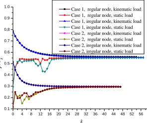
) are studied, and its geometrical size and the loading arrangement are shown in Fig.5(a). In our numerical computation, 661 regular and irregular nodes as shown in Fig.5(b) and Fig.5(c) are respectively used to discretize the structure, and the following two loading cases are taken into account: (a) Case 1, only pure tension load is applied, that is

p

_N

≠

0

and ; (a) Case 2, both tension and bending moment are considered, that is

M

0

p

=

N

0

p

≠

and

p

M

≠

0

.

N p

M

p

(a) geometrical sketch (b) 661 regular nodes (c) 661 irregular nodes Fig.5 Geometrical sketch and nodal arrangements of grooved rectangular plate

(9)

values after some iterative steps and the divergent situations do not occur, which all reveal the reliable numerical stability of present solution method.

Table 1: Limit loads of grooved rectangular plate (p /σs)

Present Loading case Tran et al.

(2010)

Casciaro and Cascini (1982)

Yan (1997)

Vu

(2001) _{regular nodes irregular nodes}

Case 1 0.556 0.568 0.558 0.557 0.560/0.556 0.555/0.551

Case 2 0.278 --- --- --- 0.298/0.296 0.296/0.294

Work:0.00 90.62 181.24 271.86 362.48 453.10 543.72 634.34 724.96 815.58 Mises: 0 4051514 810302912154543 16206057 20257571 24309086 28360600

(a) plastic dissipation work rate for Case 1, 10 J6 (b) von Mises’ equivalent stress for Case 1, Pa

Work:0.0049.7199.41 149.12 198.82 248.53 298.23 347.94 397.64 447.35 Mises: 0 3967014 793402911901043 15868057 19835071 23802086 27769100

(c) plastic dissipation work rate for Case 2, 6 (d) von Mises’ equivalent stress for Case 2,

10 J Pa

Fig.6 Distributions of plastic dissipation work rates and von Mises’ equivalent stresses for grooved rectangular plate at plastic limit states

0 4 8 12 16 20 24 28 32 36 40 44 48 52 56 60 0.1

0.2 0.3 0.4 0.5 0.6 0.7 0.8 0.9 1.0

p

/

σs

k

Case 1, regular node, kinematic load Case 1, regular node, static load Case 1, iregular node, kinematic load Case 1, iregular node, static load Case 2, regular node, kinematic load Case 2, regular node, static load Case 2, iregular node, kinematic load Case 2, iregular node, static load

(10)

CONCLUSION

A novel numerical iterative algorithm for the limit analysis of plane structures is developed in this paper, which is based on the Koiter’s kinematic theorem and the natural element method. The relevant mathematical programming formulation for upper bound limit analysis of plane stress problem is discretized in the framework of NEM, where the kinematically admissible velocity fields are approximated by the Laplace shape function, and the plastic incompressibility condition is handled by introducing a constant matrix to modify the goal function. A direct iterative formula is constructed to linearize the goal function and to calculate the kinematic load multipliers. The stress field derived from the constructed iterative formula is used to estimate the static load multipliers according to the lower bound theorem of plastic limit analysis. The solution algorithm has simple formulation and is easy for implementing. In our provided examples, the numerical results are good agreement with those available solutions, the distributions of plastic dissipation work rates and von Mises’ equivalent stresses can really reveal structural failure modes and stress states at the plastic limit states, the influence of irregular discretized nodes on the numerical results is not distinct, the iterative curves for the kinematic and static limit loads fast converge to very close steady values after some iterative steps, which all illustrate the developed algorithm in this paper is a valid, accurate and stable numerical tool to estimate the limit loads of plane structures.

REFERENCES

Braun, J., Sambridge, M. (1995). "A numerical method for solving partial differential equations on highly irregular evolving grids". Nature, 376,655-660.

Casciaro, R., Cascini, L. (1982). "A mixed formulation and mixed finite elements for limit analysis". International Journal for Numerical Methods in Engineering, 18,211-243.

Chen, G., Liu, Y.H. (2006). Numerical theories and engineering methods for structural limit and shakedown analyses, Science Press (in Chinese).

Chen, H.F. (1998). "Numerical methods for limit analysis and reference stress determination of structures under multi-loading systems and their engineering applications" PhD thesis, Tsinghua University, Beijing, China.

Cueto, E., Sukumar, N., Calvo, B., Martinez, M.A., Cegonino, J., Doblare, M. (2003). "Overview and recent advances in natural neighbour Galerkin methods". Archives of Computational Methods in Engineering, 10(4),307-384.

Sukumar, N., Moran, B., Semenov, A.Y., Belikov, V.V. (2001). "Natural neighbour Galerkin methods". International Journal for Numerical Methods in Engineering, 50(1),1-27.

Tran, T.N., Liu, G.R., Nguyen-Xuan, H., Nguyen-Thoi, T. (2010). "An edge-based smoothed finite element method for primal-dual shakedown analysis of structures". International Journal for Numerical Methods in Engineering, 82(7),917-938.

Vu, D.K. (2001). "Dual limit and shakedown analysis of structures" PhD thesis, Universite de Liege, Belgium.

Yan, A.M. (1997). "Contribution to the direct limit state analysis of plastified and cracked structures" PhD thesis, Universite de Liege, Belgium.

Zhang, X.F. (2002). "Lower bound limit and shakedown analysis of structure by the boundary element methods" PhD thesis, Tsinghua University, Beijing, China.

Zhou, S.T., Liu, Y.H. (2012). "Upper-bound limit analysis based on the natural element method". Acta Mechanica Sinica, 28(5),1398-1415.