Analysis of repeated measurement data using the nonlinear mixed effects model

ANALYSIS OF REPEATED MEASUREMENT DATA USING THE NONLINEAR MIXED EFFECTS MODEL

by

Marie Davidian and David M. Giltinan

Institution of Statistics Mimeograph Series No. 22~5 June, 1992

SERIES David M.Giltinan

(

#2225 A ANALYSIS OF REPEATED"

MEASUREMENT DATA USING THE NONLINEAR MIXED EFFECT

MODEL

j

.,

The Librnry of tile DeJl8rtment of St1!!istics North Carolina Stale Universit~

Analysis of Repeated Measurement Data

Using the Nonlinear Mixed Effects Model

Marie Davidian

*

Department of Statistics, Box 8£03, North Carolina State University, Raleigh, NC 27695 (U.S.A.)

David M. Giltinan

Biostatistics Department, Genentech, Inc., South San Francisco, CA 94080 (U.S.A.)

CONTENTS

*

Abstract

1 Introduction 2 Examples

2.1 Bioassay for relaxin by RIA

2.2 Water transport kinetics of high flux hemodialyzers 2.3 Pharmacokinetics of cefamandole

3 The nonlinear mixed effects model 3.1 Motivation and description 3.2 Inter-individual variability 3.3 Intra-individual variability 3.4 Summary

4 Overview of methods 4.1 Introduction

4.2 Methods based on individual estimation 4.3 Methods based on linearization

4.4 Other methods 5 Examples revisited

5.1 Bioassay for relaxin by RIA

5.2 Water transport kinetics of high flux hemodialyzers 5.3 Pharmacokinetics of cefamandole

6 Conclusion References

Corresponding author

1 1

2

2

3

4

4 4 5 8 8 9 9

10

13 17 18 18

20 22

.4

Situations in which repeated measurements are taken on each of several individuals arise in many areas of application. These include assay development, where dose-response data are available for each run in a series of assay experiments; pharmacokinetic analysis, where repeated blood concentration measurements are obtained from each of several subjects; and growth or decay studies, where growth or decay are measured over time for each plant, animal, or other experimental unit. In these situations, the model describing the response is often nonlinear in parameters to be estimated, as in the case of the four-parameter logistic model frequently used to characterize dose-response relationships for RIA or ELISA. Furthermore, response variability typically increases with level. Objectives of an analysis vary according to application: for assay analysis, calibration of unknowns for the most recent run may be of interest; in pharmacokinetics, characterization of drug disposition for a patient population may be the focus. The nonlinear mixed effects model has been used to describe repeated measurement data for which the mean response function is nonlinear. In this tutorial, the model is motivated and described, an overview of methods for estimation and inference in the context of the model is given, and some of the methods and analyses possible are illustrated by application to three examples from the fields of assay development, pharmacokinetics, and water transport kinetics.

1. INTRODUCTION

Data consisting of repeated measurements taken on each of a number of individuals

arise in areas such as assay development, pharmacokinetics, and studies of growth and

decay. Here, the term "individual" may refer to experiments, subjects, plants,

laboratories, devices, etc., and repeated measurements on an individual may be taken

over time, dose, or some other set of conditions. The relationship between response, y, and the repeated covariate, x, is often nonlinear in its parameters. For example, assay

data frequently conform to the four-parameter logistic model

(1)

where x IS dose. Single-dose drug kinetics are commonly characterized by

polyexponential functions based on compartment models, for example,

(2)

where x is time. A common feature in both of these contexts is a heterogeneous pattern

of variability for measurements within an individual (assay run, subject) which is

systematically related to overall response level.

The goals of an analysis will vary depending on the area of application. For example:

•

In

assay analysis, once assay procedures have stabilized, the main objective is

calibration of unknown samples for the current run. Data from each run in the

.-characterization of the pattern of intra-assay variation is crucial for appropriate calibration inference, this is an important objective in the analysis of assay data.

• In pharmacokinetic studies, repeated plasma concentration measurements are

collected from subjects following single or multiple dosing. In pilot experiments on

volunteers, several measurements are collected from each subject, and these are

used to establish an appropriate kinetic model, obtain preliminary information on

values of the pharmacokinetic parameters, and assess intra-subject measurement error, such as that due to the assay used to process blood samples. Investigation of

kinetics in a more extensive patient population relies on clinical data, and only a

small number of measurements are usually available from each subject. Interest in

this setting focuses on estimation of "typical" values for the pharmacokinetic

parameters, their relationship to individual attributes such as weight or age, and

the variation in the patient population. This information may be used subsequently in the adjustment of individual dosage schedules.

In both of these settings, a goal of the analysis is to characterize inter- and

intra-individual variation. Analysis should be conducted in a setting which recognizes the

existence of these two sources of variation in repeated measurement data and allows

them to be evaluated. A natural parametric framework which accommodates these

features is the nonlinear mixed effects model. In this tutorial, we discuss this model and show how it provides a basis for inference in several application settings. In Section 2

we introduce three examples from the fields of assay development, water transport

kinetics, and pharmacokinetics. Section 3describes the model framework. An overview of approaches to estimation and inference is provided in Section 4, and some of these techniques are illustrated by application to the examples in Section 5.

2. EXAMPLES

2.1 Bioassay of relaxin by RIA

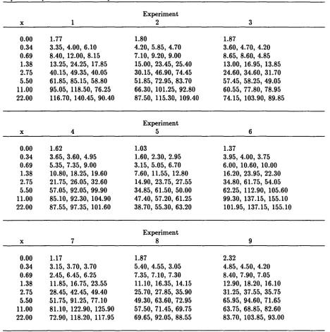
Table 1 shows dose-response data obtained for standard concentrations in nine runs of a bioassay for the therapeutic protein relaxin [1]. The assay is based on increased

generation and release of intracellular cAMP by normal human uterine endometrial cells

in the presence of relaxin. For each of the nine runs, triplicate cAMP measurements were determined by RIA for each of seven known relaxin concentrations. A single

control measurement was also available for each plate. Figure 1 illustrates

concentration-response data for the standard for two of the runs, where response at zero

four-

.-·"'

parameter logistic model (1) is a reasonable representation of dose-response for a given

run; however, parameters such as logED50

(/33),

background

(/32),

and mean response at

infinite dose

(/31)

vary from run to run. Variability in measured cAMP levels increases

with response level for a given run (see [2]) in a way that is similar across runs.

The objective of an analysis is calibration of unknowns for the most recent run. As

described in [3] and [4], accuracy of calibration confidence intervals and precision

profiles for a run will depend critically on how one characterizes this increasing

intra-assay variation. In Section 5, we will show how using the nonlinear mixed effects model as a framework for analysis allows this variation to be characterized using data from all

nine runs, resulting in improved calibration inference.

2.2 Water transport kinetics of high flux hemodialyzers

In [5], data are presented from an experiment to evaluate the water transport kinetics

of high flux membrane dialyzers used for hemodialysis for patients with end-stage renal disease. Twenty dialyzers were evaluated in vitro with bovine blood at two different

blood flow rates, 200 or 300 ml/min. For each of seven values of transmembrane

pressure (mmHg) exerted on the dialyzer membrane, ultrafiltration rate (ml/hr) at

which water is removed was measured for each dialyzer. These data are given in Table

2, and profiles for each dialyzer are plotted in Figure 2.

Since the relationship is governed by protein polarization, which causes a relatively

constant ultrafiltration rate at high pressure, and oncotic pressure, a nonlinear model for

the relationship between ultrafiltration rate and transmembrane pressure x IS

appropriate [5]:

(3)

..

where

/31

is the maximum attainable ultrafiltration rate due to protein polarization,

/32

is a hydraulic permeability transport rate, and

/33

is the transmembrane pressure

required to offset patient oncotic pressure. For a given dialyzer, the seven available

observations provide enough information to fit (3) to the data for that dialyzer by

nonlinear (unweighted) least squares (LS). Figure 3 shows a plot of LS residuals against

predicted response, as described in [3], for a typical dialyzer. The "fan-shaped" pattern

is evidence that intra-dialyzer variability is an increasing function of ultrafiltration

response level.

One objective of the experiment was to contrast kinetic properties for dialyzers at the

.-incorporation of inter- and intra-dialyzer variation. 2.3 Pharmacokinetics of cefamandole

The results of a pilot study to investigate the pharmacokinetics of cefamandole, a

cephalosporin antibiotic, are reported in [6] and are shown here in Table 3. A dose of 15

mg/kg body weight of cefamandole was administered by 10 minute intravenous infusion

to six healthy male volunteers, and blood samples were collected from each subject at

each of fourteen time points post-dose. Plasma levels (pg/ml) for each sample were

determined by HPLC. Figure 4 plots the resulting plasma level-time profiles for each

subject and indicates that the biexponential function (2) arising from a

two-compartment model for cefamandole kinetics is reasonable, although the values of the

pharmacokinetic parameters may vary across subjects. For pharmacokinetic data, the variation associated with plasma concentrations is likely to be an increasing function of

level, in part due to the nature of the HPLC assay [7,8,9].

As discussed in Section 1, the goals of an analysis of data from a pilot study such as

this are to characterize this intra-subject variation, which is likely to be the similar for

all individuals, and to estimate the pharmacokinetic parameters. We illustrate these ideas in Section 5.

3.

THE NONLINEAR MIXED EFFECTS MODEL

3.1 Motivation and description

In the three examples in Section 2, several common features are apparent: The same

nonlinear model for the relationship between response and x is suitable for describing

data for each individual, but the values of the parameters that specify the model fully

may differ across individuals (inter-individual variation). Furthermore, the variability associated with response measurements for a given individual depends on response level

in a way that is likely to be similar for all individuals, due to, for example, properties of

an assay (intra-individual variation). Correct analysis should account for both of these

features; moreover, characterization of these features may be a goal. The following

nonlinear mixed effects model incorporates both sources of variation. The use of this

model as an analytic tool was pioneered by Beal and Sheiner [7,8,9], who recognized and

advocated the need to accommodate and assess both types of variability in

pharmacokinetic analysis. More general specifications than that presented here are

possible, and the reader is referred to the work of Beal and Sheiner for such

formulations with particular reference to pharmacokinetics.

.~

the set of conditions summarized by the vector of covariates Xij' The vector Xij

incorporates variables such as time, dose, pressure, etc. Suppose that a (nonlinear)

function

f(x,f3)

may be specified to model the relationship between Yij and Xij'

Inter-individual variability is accommodated by the assumption that, although f is

common to all individuals, the (p

xl)

regression parameter vector

13

may vary across

individuals. This is incorporated by specification of a separate (p

xl)

vector of

parameters f3i for the ith individual. For example, for the relaxin bioassay, f3i would be

the (4

xl)

vector whose components are the parameters of the four-parameter logistic model (1) corresponding to the ith run of the assay. The mean response for individual i,

given the parameter vector

f3i'

is thus E( Yij

I

f3i)

=

f(Xij,f3i)'

For a given individual, the variability in Yij may be a function of f(Xij,f3i)' For

example, variance may be proportional to a power of the mean response given

f3i'

that

is, Var(Yij

I

f3i)

= (12{f(xij'

f3i)}2/J

for some scale parameter (1 and a power 6; if () = 1, this is the constant coefficient of variation (CV) model with CV = (1. In this specification, the parameters (1 and () are common to all individuals, reflecting the belief that the pattern of variability in measurements is similar across individuals. This will be the

case if, for example, the pattern is primarily due to a (common) assay used to obtain

response measurements. In general, write Var(Yij

I

f3i)

= (12 g2{f(Xij'

f3i),6},

where the variance function g describes the common pattern of variability. Other examples of

models g for intra-individual variance are given in [3] and [9].

With these definitions, the nonlinear mixed effects model assumes that the jth

measurement on individual i can be written as

(4)

where fij is a random error with mean 0 and variance 1. We now turn our attention to

further description of the components of the model. 9.2 Inter-individual variability

In (4), inter-individual variation is modeled through the assumption of the

individual-specific regression parameter vector

f3i'

Part of the inter-individual variation in the

values of the parameters characterizing mean response may be due to systematic

dependence on individual attributes. For example, pharmacokinetic parameters are

well-known to depend on an individual's weight, disease status, and so on [7,8].

Parameters may also vary due to unexplained random variation in the population of

run-to-run variation in assay procedure.

To account for these possibilities, a model for the dependence of f3i on individual attributes and random variation may be specified. The simplest such model is that in

which inter-individual variation is assumed to be entirely due to unexplained

phenomena:

(5)

.-."

where I is a (p xl) vector of fixed parameters and Zi is a random vector assumed to

arise from a population with mean Op, a (p X 1) vector of zeros, and covariance matrix ~. Equation (5) states that the f3i vary in the population of individuals about the value " their mean, and the variation in the population is described by the matrix~. The

diagonal elements of ~ characterize the variance of each component of the f3i about " and the off-diagonal elements describe how the components vary together (covariance).

A more complicated model allows for dependence on both random and systematic

phenomena. For example, in the dialyzer study of Section 2.2, water transport kinetics may be thought to vary among dialyzers in part because of flow rate and in part

because of natural variation expected to occur among the devices. Both possibilities can

be taken into account by assuming that

f3i = 1200

+

Zi ifdialyzer i is used with flow rate 200 ml/min,

f3i = 1300

+

Zi if dialyzer i is used with flow rate 300ml/min,

(6)

where 1200 and 1300 are (3 x 1) vectors describing the central tendency of the 3 kinetic parameters in (3) for the populations of dialyzers operated at flow rates 200 ml/min and

300 ml/min, respectively. The random component zi is again assumed to have zero mean and covariance ~, so that random variation in both populations is assumed to be

similar. Model (6) may be written compactly in the form of a "linear regression"

model:

f3 .

_I = W·,oy_{I I}

+

z·_" (7)

where

I

=

[,ioo, IIoo]T,

that is, the (6 x 1) vector with 1200 and 1300 stacked, and Wi is a (3 x 6) "design" matrix such that

Wi

=

[13103,3] ifdialyzer i is used with flow rate 200 ml/min,

."

where Ir is a (r X r) identity matrix and Or•• is a (r X s) matrix of zeros. Note that, under model (7), a comparison of kinetics between the 2 flow rates could be made by comparing 1200 and 1300' the "typical" kinetic parameters for each population.

As another example, consider a situation in which pharmacokinetic parameters are

thought to depend systematically on individual attributes. For specificity, suppose that f3i is a (2 x 1) vector whose components are clearance CLi and apparent volume of

distribution Vi' Suppose that clearance is thought to be a linear function of an

individual's weight Wi' Random variation in pharmacokinetic parameters often increases with their magnitude [7,8]. These features are accommodated by the following

models for CLi and Vi:

(9)

where 1 = bl, 12' 13]T and Zi = [Zil, Zi2]T. Ifthe components of the random vector Zi have symmetrically-shaped distributions and Zi is centered at 0 with covariance ~, then

the distributions of CLi and Vi will be skewed with constant coefficient of variation. To

illustrate further, suppose that f3i contains a third component kai, the first-order

absorption rate constant, but there is reason to believe that this parameter varies little

across individuals. This feature may lead to the assumption that kai is fixed across

individuals, so a specification for kai should include no random variation:

(10)

Writing 1

=

bl,12,13,,4]T and Zi

=

[Zil,zi2]T, the model for f3i

=

[CLi' Vi,kadT may be written compactly as

(11)

where h is the trivariate-valued function given in (9) and

(10).

Note that because kai is

assumed to be fixed, the dimensions of 1 and Zi need not be the same.

Equation (11) is a general model describing the variation in parameter values across

individuals. We shall use this notation for general models for

f3i,

where Wi is a vector or matrix containing information on individual attributes such as weight or group, and,

in accord with usage in the pharmacokinetics literature, refer to h as the inter-individual

regression model. Note that this general specification subsumes simpler ones such as (5)

3.3 Intra-individual variability

In the nonlinear mixed effects model (4), intra-individual variation is modeled

through the intra-individual variance function g, the parameters ( j and (J, and the

random errors fij. This variation is interpreted as that associated with measurements on a given individual i. It is often reasonable to assume that measurements within a given individual are statistically independent, reflected in the model by the assumption

that the random errors fij are independently distributed.

In some settings, this assumption may not be realistic. When measurements are

taken on a given individual at closely space time points, it is likely that successive

measurements may be correlated; that is, responses taken close in time may be "more alike" than those taken far apart. This situation may be accommodated by assuming

that the fij are not statistically independent but are correlated in some specifiable way.

An example is to assume that the random errors follow an autoregressive process of order 1; see [10, ch. 6]. In practice, however, it is often assumed that the fij are independent, in part because successive time points are thought to be sufficiently far

apart so that such serial correlation is negligible. Another justification is that, in (4),

the fact that the common (random) (3i appears in f and g will have the effect of

inducing a relationship among measurements on individual i. This is considered to be

adequate to account for any association that may actually exist among measurements

on an individual

[11].

Based on these considerations, we assume for our discussion that the fij are

independent. The methods for estimation in the nonlinear mixed effects model in

Section

4

may be generalized to the case of correlated fiji see

[1]

for details.

3.4 Summary

For convenience, we summarize in vector notation the version of the nonlinear mixed

effects model that forms the basis for our discussion. Let Yi

=

_{[Yil' ... , Yim.]T, fi((3i)}

=

I

[f( xiI, (3i), ... , f( xim.' (3i) ]T, and fi = [fil' ... , fim.]T be the (mi xI) vectors of responses,

I I

mean response functions, and random errors, respectively, for individual i. Let G_i((3i,9) be the (mi x mi) diagonal matrix with diagonal elements gij

=

g{f(xij' (3i),9}. With these definitions, we write the nonlinear mixed effects model as

z· '"I

Yi = _fi((3i)

+

( jGi((3i, 9) fi (mi xI),

(3i = _{h(Wi", Zi)} (p xI),

(0, E)

(M

x 1) distributed independently of fi '" (0, 1_{m.) (mi} xI),

I i

=

1, ...

,n,

j = 1, ... , mi'

.'

where the notation" '"

(a, B)"

means "distributed with mean

a

and covariance matrix B," M is the dimension of the random components Zi for the inter-individual regression model h, and the assumption that Zi and €i are distributed independently reflects the

belief that the mechanisms governing the 2 sources of variation operate independently. This is a version of the model discussed by several authors [4,5,7,8,11,12].

4. OVERVIEW OF METHODS

4.1 Introduction

In the context of the nonlinear mixed effects model (12), questions of interest may be

formulated in terms of the components of the model. In assay analysis, for example, the objective is individual inference for a given run i; in particular, this involves estimation of

f3i

characterizing the standard curve for run i and estimation of 9 (which will determine the weighting scheme for this fit), calibration of unknown samples based

on this estimate of

f3i,

and construction of calibration confidence intervals and precision

profiles (which will depend on the estimates for

f3i,

u, and 9). In pharmacokinetic analysis, one goal is population inference; this involves determination of an appropriate

function h and estimation of , and I:, all of which characterize the population of subjects. Another aim in pharmacokinetic analysis is individual inference - estimation

of

f3i

for a particular individual. Under the model, it seems reasonable to expect that

the information available from all individuals will be useful for both population and

individual inference. This is in fact the case - estimates of

f3i

and 9, for example, that

make use of information from all subjects are preferred to those based on data from

individual i alone [4].

The model (12) acknowledges that inter- and intra-individual variation should be

considered in an analysis of repeated measurement data. As pointed out by Beal and

Sheiner [7], early attempts at analysis of these data did not take both features into

account. In particular, the popular method of analysis was essentially to assume that

the model for yij is

(13)

where

13

is common to all individuals. Estimation of

13,

the vector of model parameters

(assumed the same for all individuals), was accomplished by ordinary nonlinear LS

based on (13), "pooling" the data from all individuals. This is referred to as the "naive pooled data" method [7,8], since it ignores variation across individuals, Estimates of

13

inter-10

individual variability is possible. This method is not recommended [8].

The nonlinear mixed effects model (12) is complex, since, in order to account for the

two sources of variation, two random components, Zi and fi, are required. The random

component zi appears in the model through the nonlinear functions hand f; thus, the effect of inter-individual variation on response measurements is complicated. Standard

statistical methodology such as maximum likelihood (ML) estimation or LS is

predicated on the ability to specify a distributional model for a response vector Yi. In this situation, because of the complex way in which Zi appears in the model, it is not

possible to write down a distribution for yi, even if it is assumed that both Zi and fi are

normally distributed. Thus, standard techniques may be difficult to implement. As a

result, many of the methods that have been proposed for analysis of (12) are based on

approximations which allow a distribution to be specified for Yi'

We now review some methods for estimation of " E,

f3i,

(7, and 9 for the nonlinear

mixed effects model (12) that have been suggested in the literature. The methods we

describe represent only some of procedures that have been proposed, and references to

other methods are given.

4.2 Methods based on individual estimates

One approach to an approximation based on (12) is based on the ability to construct,

for each individual, estimates

f3i

for

f3i.

These estimates form the basis for estimation

of " E, (7, 9 and, in some cases, improved estimates for

f3i.

Intuitively, for this idea to

be successful, sufficient data must be available on each individual for suitable

f3i

to be

obtained. These methods are referred to as two-stage methods in the pharmacokinetics

literature [7,8,12] since the idea consists of two stages: construction of

f3i

and

subsequent estimation of other parameters.

The standard two-stage (STS) method [for example, 12] treats estimates

f3i

as if they were the true

f3i'

In the simplest case of (5), estimates for , and E would be

constructed as

(14)

the sample mean and covarIance of , and E, respectively. Although simple, these

estimators take no account of the uncertainty associated with estimation of

f3i

by

13:-The result is that the estimator for E can be very biased and imprecise. Furthermore,

no attempt to improve on

f3i

by taking advantage of all available information is made.

These estimators are generally regarded as undesirable [4,7,8,12].

0"

o·

into account. Several methods to do this have been proposed [7,8,12,13]; we describe

explicitly one such method, referred to in [12] as the global two-stage (GTS) method.

The method is given in terms of a linear inter-individual regression model as in (7). An assessment of the uncertainty of estimation in

13;

may be obtained by appealing to large sample theory for nonlinear regression, as described in [3, sec. 3.2]. The theory

states that, for large numbers of observations (in our case, large mi)' the sampling

distribution of an estimator

13:

is p-variate normal with mean l3i and some covariance matrix Vi' say, where the form of Vi is determined by the nature of f and

13:

and depends on

l3i.

In practice, Vi is estimated by replacing parameters by estimates where

they appear; henceforth, assume that Vi refers to such an estimate. If this theory is relevant, we have that, given

l3i,

13:

is approximately normally distributed with mean l3i and covariance Vi' write

13:

Il3i '" N(l3i, Vi). If we are further willing to assume that l3i is normally distributed with mean W(Y and covariance E, as suggested by (7) for normal

Zi, then it follows that

13: '"

N(W(y, Vi

+

E). This argument thus leads to a distributional assumption about

13:,

suggesting that standard approaches to estimation of I and E may be used, treating the

13;

as "data." The GTS method estimates I and E by ML estimation based on this normal distribution and is implemented by a two-step

iterative algorithm [1,12] which produces as a byproduct "refined" estimates of l3i that make use of information from all individuals. The algorithm may be started by using

initial values for I and E from (14). At iteration

(k+1):

(1) Produce refined estimates of

l3i:

(2) Obtain updated estimates of I and E:

~ _ ~ Q(k) a(k+l) I(k+l)-.L." • fJ. ,

.=1

Q

(k)• = (

.=1

. L . " .~

w

r

t-

( k ) .

1w.)-lw

•

r

t-

(k)'

1.

Iteration continues until the algorithm converges to final estimates 1',

t,

and Pi. Note that the "refined" estimates in (15) have the form of a "weighted average" of the

12

fact empirical Bayes estimates for

l3i;

that is, ~i is the mean of the distribution of l3i giventhe data {Yij}, where '1 and ~ have been replaced by the current estimates [12].

By standard statistical theory for ML estimation, estimates of the uncertainty

associated with, for example,

:y,

may be obtained. An estimate of the covariance matrix for

:y

is

l:1

=

{.f:

Wr

(V_i-

1

+E-

1

)-lW_i

}-1

.=1

(16)

([1]) and may be used to construct hypothesis tests about '1, as described in Section 5. Two-stage methods are based on separate estimates

13:

for each individual. Thus, it is not straightforward to use these methods when one of the components of l3i is taken to remain constant across individuals, as in the pharmacokinetic example (10).

For any two-stage method, the quality of the estimates of '1 and ~ will depend on the quality of the estimates

13:.

If intra-individual variance is not constant but varies according to the function g with response level, using ordinary LS estimates for

13:

will

be undesirable, because LS estimates will be inefficient relative to estimates based on

weighted least squares (WLS)

[3].

The weighting scheme to be used will depend on

what is known about the function g. As is frequently the case, one may be able to

specify a function g which describes the pattern of variation, but the value of 9

providing a full characterization is unknown and must be estimated from the data

[3].

Ifit is realistic to assume a common pattern of variation for all individuals, as in (12),

it makes sense to use the data from all individuals to estimate 9 (and u) rather than to estimate separate values for each individual.

This idea is the basis for the following proposal for obtaining

13:

advocated in

[4].

We

first review estimation for data from a single individual. As described in

[3],

for a given

individual, variance function estimation procedures use residuals from a previous fit as

the basis for estimation of u and

9.

Two such procedures are described in

[3,

sec.

4]

and

are incorporated into an iterative generalized least squares (GLS) algorithm for

estimation of the individual's regression parameter. This algorithm may be summarized as follows for use with data from a singleindividual. For individual i:

1. Obtain the LS estimator

13:(0)

and set k = O.

2. Given 13:(k), minimize the objective function Oi(I3:(k),u, 9) in u and 9 to obtain

ilk>,

where Oi(l3i,u,9) is an objective function such as

PL (_ifJi,U,17

R

a)

=.-::-

~

({Yij - f(xij,l3i)P_{22{f( .. R.)a}+ogu g}I [ 2 2{f(_Xij,fJi,17

R)

a}l)

_,

J - 1 U g X.J,fJ.,17

and form estimated weights w~~)

=

l/g2

{f(Xii'

fJ:(k»), e(k)}.

3. Obtain the GLS estimator of fJi by WLS with weights w~~). Set k = k+1, let

fJ:(k)

be this GLS estimator, and return to step 2.

The objective functions for estimation of ((1,8) in step 2 are motivated in [3,4]. The

scheme may be iterated a fixed number of times or until convergence, see [3].

In [4], the GLS algorithm is extended to allow estimation of (1 and (J based on data from all individuals:

1. For each individual i, estimate fJi by LS. Call these n estimates

1':(0),

i = 1, ... , n.

2. Minimize in (1 and (J

where 0i is one of the objective functions in (17), obtaining

e(k).

For each

individual i, form estimated weights w~~)

=

l/g2{f(Xii'

fJ:(k»), e(k)},

i

=

1, ... , n.

3. For each individual i, obtain the GLS estimator of fJi by WLS with weights w~~). Set k = k+1, let

fJ:(k),

i = 1, ... , n be these GLS estimators, and return to step 2.

In step 2, information from all individuals on the (common) intra-individual variance

structure is used to estimate ((1,8) by pooling information across individuals. Since the

objective function is simply the sum of the objective functions for all individuals, minimization is no more difficult than for data from a single individual only. See [3]

and [4] for details on implementation with standard software. As in the case of individual data, this scheme is iterated a fixed number of times or until convergence.

The final estimates

fJi

from this scheme are proposed in [4] as input to one of the

procedures such as GTS for estimation of I and~. These

fJi

are to be preferred to

those based on a separate estimate for 8 for each individual because they are likely to be

more precise, since they are based on a weighting scheme that takes advantage of the

information from all individuals through the "pooled" estimation of (1 and 8.

To summarize, the procedure is: (1) Obtain

fJi

by the GLS algorithm based on pooled estimation of ((1,(J), and use these estimates to form Vi; (2) Use

fJi

and Vi as input to a scheme such as GTS to estimate (I,~) and obtain refined estimates of fJi if desired. These "pooled two-stage" (PTS) methods may be used when sufficient data are available to obtain estimates

fJi

from each individual.

4.9 Methods based on linearization

model is based on linearization of the model (12) by a Taylor senes III the random effects Zi' This idea was first advocated by Beal and Sheiner [7,8]. Under the

assumption that Zi'" (0, E) and fi'" (0, 1m .), they proposed that the Taylor series be

I

taken about Zi

=

0, leading to the approximate model

where Di(Wi",')

=

Xi{h(Wi",'

n

Hi(Wi", '), Xi(·) is the (mi x p) matrix of derivatives of fi(Pi) with respect to Pi, and Hi(Wi", . ) is the p x

M

matrix of partial derivatives of h(Wi' "Zi) with respect to Zi' This approximation implies

E(Yi) =fi{h(Wi",

On;

COV(Yi)":'" Di(Wi", 0) EDT(Wi", 0)

+

(]"2GH h(Wi", 0), 8}. (19) Ifone assumes that the random components Zi and fi are normally distributed, and if (18) is treated as exact, then the Yi have mi-variate normal distributions with mean and

covariance given in (19). This approximation is the basis for the suggestion of Beal and

Sheiner to obtain estimates of (" E, (]", 8) by maximizing in these parameters the normal

likelihood for the data vectors Yi, i

=

1, ... , n, corresponding to these assumptions. In the pharmacokinetics literature, this procedure is referred to as the "First-Order"

method, and the estimation scheme corresponding to normal ML is referred to as

Extended Least Squares (ELS) [7,8,9]. The method is implemented in the software

package NONMEM [14]; the reader is referred to this documentation for computational

details. The individual Pi may be estimated by an empirical Bayes approach as well

[14]. NONMEM is widely used in the analysis of population pharmacokinetic data. For

some problems, this approach can be computationally intensive.

Recently, Vonesh and Carter [5] have proposed an alternative to the ELS method

which is also based on the linearization (18) but is computationally simpler. In [1],

their method has been modified to incorporate a variance function g and estimation of

fJ. The procedure is a four-step iterative algorithm in the spirit of GLS. The second

step is based on the idea that, if , _{were known in (18), [Yi - fi{h(Wi",}

On]

= Di(Wi", 0) Zi

+ (]"

Gi{h(Wi", 0),fJ} fi is a weighted linear "regression model" for individual i with "regression parameter" Zi' "design matrix" _{Di(Wi", 0), and} . "covariance matrix" (]"2 GHh(Wi", 0), 8}.

Step 2. _{Form e;=y;- f;{h(W;,1'(k),On, let D; = D;(Wi,1'(k)' 0), and iterate the} following steps:

(i) Let j = 0. For each individual, obtain an initial estimate of Z;, z~j) =

A '" 1 A

(D;D;)- Diei'

(ii) Form "residuals" I; = e;-D;z~j) and estimate (0",8) by (17,8) jointly maxImIZIng

(iii)

where

0;

is a suitably chosen objective function.

Form

G;

= G;{h(W;,1'(k)'0),

8},

update the random effects estimates for each individual by z~j+I) =

(D;Gi1

D

_i)-l

D;Gi1e;,

and let j = j+ 1. Return to (ii). Call the final estimates from this process z~k), u(k)' 8(k)' and let

G;

= G;{h(Wi,1'(k)'0),8(k)}

Step 3. Let Szz = (n-l)-I

f:

(z~k)_z)(z~k)_Z)T

,z

= n-I

f:

z~k), and estimate ~ by

i=I i=I

Step 4.

. . ..

.

mInImIZIng In ,

n A -1

t=

[Yi - f;{h(Vi", On]T(U;)(k) [Yi - f;{h(Wi", On]·

1=1

Let k = k+1 and return to Step 2.

If _Gi

=

1_{m .} no iteration is required within Step 2. In general, Step 2 is not too

1

intensive since the "regression" fits are linear, and the process often converges after a few iterations. As in Section 4.2, at least one iteration of the entire algorithm should be taken; results often stabilize after three to five iterations. At the end of Step 4, individual estimates may be constructed as ,8~k+1) = h(W;,1'(k+1)'z~k)).

16

(20)

Maximization of these objective functions in step 2(ii) can be accomplished using standard software, see [1,3,4].

The covariance matrix of 1'(k+I) obtained at the end of the Step 4 can be estimated by

(21)

where Xi IS Xi evaluated at _h(Wi,1'(k+1),0) and Vi

Di(Wi,1'(k+I),O)t(k)Di(Wi,1'(k+I),O)T +

u~k)GHh(Wi,1'(k+I),0),9(k)}'

This method may be used when information from each individual is sparse as long as mi ~ M.

Lindstrom and Bates [11] suggest that the approximation based on Zi ==

°

can be improved and propose a computational method based on a Taylor series of (12) about Zi

=

zi,

for

zi

"near" Zi' This yields the approximate model and moments

Yi == fi{h(Wi, /"

zi)} -

Di(Wi, /" z:)

zi

+ Di(Wi, /" zi)Zi + 0"Gi{ h(Wi, /" zi), 8} €i;

E(Yi) ==fi{h(Wi, /"

zi)} -

Di(Wi, /" zi)

zi ,

Cov(Yi) == Di(Wi, /" zi) EDT(Wi, /" z:) + 0"2GH h(Wi, /" z:), 8}. (22)

To base estimation of (/" E,0",8) on this approximation, it is necessary to have

available a value for

zi.

Lindstrom and Bates propose an iterative scheme in which an estimate of Zi is obtained at each iteration. This estimate is inserted in the expressions in (22), and updated estimates of (" E,0",8) and Zi are obtained. The iterative

computation is fairly complex; we only summarize the basic idea. At iteration

(k+1):

(1) Given current estimates 1'(k)' t(k)' u(k)' 9(k)' and

z~k),

obtain updated estimates

z~k+I) of Zi: maximize the likelihood for Zi given the dataYij under the assumption

that the Zi and €i are normal, obtaining the estimates

Z(k+I) =

[u-

2 ]).{G~}-1]).+ t ] -1 X

, (k) " , (k)

( A-2DA {GA2}-I[ f{h(W A A(k»)}+D A

A(k»)

O"(k) i i Yi- i i'/'(k)'Z' i Z, '

where

D

i

=

Di(Wi , 1'(k)'

z~k»)

and

G

i

=

Gi {h(Wi,1'(k)'

z~k»),

9(k)}'

17

estimates 1'(k+l)' t(k+l)' U(k+l)' 8(k+l) maxImIZing In

b,~,cr,8)

the normal likelihood for the data vectors Yi' i = 1, ... , n, with means and covariance matrices

f .{h(W. 'V zA(k+l))} _ nA.zA(k+l) nA~nAT+ 2G2{h(W A A(k+l)) Ll}

• 11 " • . . , i~ i cr i i''(k)'Z. ,u ,

respectively.

We refer the reader to [11] for full details and computational strategies. In the above,

we have modified the Lindstrom and Bates proposal for nonlinear h and to incorporate

estimation of 8 in a variance function depending on f3i. At the end of (2), estimates of the individual f3i may be obtained as ~~k+l)

=

h(Wi,1'(k+l),z~k+l)).

4.4

Other methods

As pointed out in Section 4.1, the major classes of methods that we have discussed

are based on approximations or individual estimates because the complexity of the

model

(12)

makes the use of standard methodology difficult. This is because it is not

possible in general to specify a distribution for the data vectors Yi, even with

distributional assumptions for Zi and fi' We now examine this problem more closely. If we were to assume, for example, that the fi are normally distributed, this would imply

that, given f3i (and hence, given Zi), Yi are normally distributed with mean vector fi(f3i) and covariance matrix cr2GHf3i' 8). Writing </>(a, B) to be the normal density with mean

vector a and covariance matrix B, if zi is assumed to be distributed with some density

t/J( .

I

~) depending on ~, the exact likelihood for the response vector yi is

(23)

the likelihood for the entire data set would be the product of n such integrals, one for

each individual. Even if

t/J

is the normal density </>(0,~), this integral is not analytically

tractable for general functions f, g, and h.

Recently, methods have been proposed which, under various assumptions, represent

attempts to perform this integration in order to estimate the parameters. A full

description of these methods is beyond the scope of our discussion; we provide only a

brief summary and references.

Gelfand, et al. [15] take a full Bayesian approach to the nonlinear mixed effects

model. They assume that Zi and fi are normally distributed random vectors and place

In this framework, several integrations, including that in (23), need to be performed. A computationally intensive Gibbs sampling algorithm is advocated to perform these

integrations; a description of this approach and specific details are given in [15].

Mallet et al. [16] note that the assumption that Zi are normally distributed may be

questionable in population pharmacokinetic analysis. They propose estimation of the

density of Zi, "p, in (23) by a nonparametric method. The parameters, and u are then

estimated by integrating (23) with this estimate inserted for"p. Since the estimate for "p

consists of a finite number of points, the integral becomes a sum, which may be

evaluated easily. See [16] for a full exposition.

Davidian and Gallant [17] also eschew the standard normality assumption for "p.

They propose a different nonparametric estimator for "p which is not a finite number of

points but rather is a smooth function of z. By using numerical integration, they compute the integral (23) and estimate "p, " ~, u, and 9 simultaneously. The form of

the estimator for "p includes

4>,

the normal density, as a special case.

The methods in this section can involve fairly substantial computational costs. For

all methods, including those discussed in Sections 4.2 and 4.3, very little is known about relative performance. This issue is a basis for current research.

5.

EXAMPLES REVISITED

5.1 Bioassay of relaxin by RIA

Calibration of unknown samples for the current run of a cell-based bioassay such as

that for relaxin is always based on the standard curve for that run. As noted in Section

2.1, accurate characterization of intra-assay variability in the response is essential for

assessing the precision of calibration. We now illustrate how this issue may be

addressed for the relaxin bioassay within the nonlinear mixed effects model framework.

Variability in assay responses is an increasing function of response level, and a

standard model for characterizing this feature is the power of the mean variance

function [2]. That is, for run i,

g{f(xij, (3i), 9}

=

f(xij, (3i)(} (24)

for some power 9. It is commonly acknowledged that for many assays, usual default choices for this power, such as 9

=

0.5 or 1.0, may be inappropriate [18]. Thus, one

objective of an analysis is to determine an appropriate value for 9 for the ith run. The choice of 9 often has little impact on the estimated values of the parameters of the

19

calibrated values. However, the value of 8 used directly affects one's ability to assess

the precision of calibration accurately, as the following development shows.

A standard technique for evaluating intra-assay precision associated with calibration

of an unknown sample for a given run is to construct a precision profile

[19].

Such a profile is a plot of estimated precision of an estimated concentration against concentration across the assay range. To illustrate one way to construct a precision

profile, let d be the inverse of the four-parameter logistic function, that is, x

=

d(y,13)

=

exp[133

+

log{(132 -

y)j(y -

131)}

j

134],

and let dy(y,13) and the p-variate vector-valued

function d,a(y,13) represent the derivatives of d with respect to y and

13,

respectively.

Then if Yo is the average response for r replicates of an unknown sample for the ith run

at concentration xo, the estimated value of Xo is given by :leo = d(yo, Pi), where Pi is an

estimate of 13i with estimated covariance matrix Vi. An estimated approximate variance for :leo may be obtained by a Taylor series:

(25)

where (0-,9) are estimates of the intra-assay variance parameters. The first term in

(25)

reflects uncertainty in the measurement Yo and will usually dominate the second term,

which corresponds to uncertainty in the fitted standard curve. A precision profile is

constructed as {Var(:leo)}1/2j:leo versus :leo. Since the first term in

(25)

depends on

(0',

8),

assessment of precision of calibration will be sensitive to the values of

0'

and 8 used.

Appropriate values for

(0',8)

in this context are often determined by estimation from

the available data, usually based on data from the current run only, using, for example,

the GLS algorithm for individual data given in Section 4.2. Although sufficient data are

available to provide reliable estimates of 13i based on data from a single run, estimates

of

(0',

8) obtained in this way are usually less reliable, mainly because estimation of

variance parameters is more difficult.

This difficulty may be avoided if one is willing to assume a similar pattern of intra-assay varability across runs. Although the values of

(0',

8) may be expected to vary

from run to run during assay development, once assay procedures have stabilized,

supposition of common values of

0'

and 8 across assay runs is not unreasonable. The

nonlinear mixed effects model

(12)

provides a framework for analysis under this

assumption, with f as the four-parameter logistic function, g the power of the mean

model (24), and h as in (5). The GLS algorithm in Section 4.2 where data are pooled

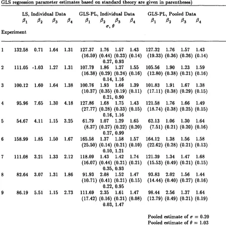
Under these assumptions, Table 4 displays the results of several fits to the relaxin

data, both separately by assay run and pooled across assay runs. Because results were

very similar for both objective functions in (17) for individual and pooled estimation, we

report results for PL only. Although individual estimates of () are fairly similar across

runs, the value for run 9 seems somewhat aberrant. This is probably attibutable to the

difficulty in estimating variance parameters mentioned above. The pooled estimate for

() based on data from all nine runs indicates that a constant CV model for intra-assay

variance would be a reasonable choice for routine use.

In Figure 5, a precision profile for a single replicate of an unknown sample is constructed based on each fit for run 9. The profile based on the LS fit is inappropriate,

since it takes no account of the nature of intra-assay variance. The profiles based on

individual and pooled GLS fits differ appreciably over a large range of concentrations,

reflecting the sensitivity of calibration inference to the method used to characterize intra-assay variability. If the model assumptions are correct, then the profile based on the pooled GLS fit will provide the most accurate assessment of precision.

More extensive analysis of this example and further discussion of issues arising in

calibration, including the use of refined estimates of f3i from GTS as a basis for

calibration, is given in [18].

5.2 Water transport kinetics of high flux hemodialyzers

An objective of the dialyzer study was to compare the kinetic properties of dialyzers operated at the two flow rates. We now address this question in the context of the

nonlinear mixed model framework, assuming the kinetic model fin

(3)

throughout.

In a preliminary analysis, Vonesh and Carter [5] determined that {33' transmembrane

pressure, was constant across dialyzers within each flow rate, although the value of

133

was likely different for the two flow rates. Thus, we follow Vonesh and Carter and

adopt the following inter-individual regression model h for the vector of kinetic

parameters f3i

=

[{3il' f3i2' f3i3]T for individual i. For dialyzer from flow rate 1,1

=

200, 300:

where '11 = ['11" '12" '131]T is the vector of "typical" kinetic parameters for a dialyzer operated at flow rate 1= 200 or 300 ml/min, and Zi = [Zil' Zi2]T is the random vector describing how the first two parameters, maximum ultrafiltration rate and permeability

transport rate, vary in both flow rate populations. This model may be written as f3i =

matrix whose columns are the first two columns of 1_{3 •}

From Figure 3, intra-dialyzer variability is an increasing function of ultrafiltration

level. To accommodate this feature, we assume that intra-dialyzer variance follows the

power of the mean model (24). In their analysis, Vonesh and Carter [5] assumed

constant intra-dialyzer variance.

The two-stage methods in Section 4.2 do not allow for the possibility that some

components of

Pi

are fixed; the methods based on linearization in Section 4.3 do

accommodate such a model. We thus used the four-step GLS algorithm given in

Section 4.3 to estimate (;,~,u, 6). Results were similar for the two objective functions

in (20); hence, we report those for PL only. The process stabilized after three iterations in that the relative change in parameter estimates between successive iterations was less

than 10 -4. The estimates are:

1

=

[4512.782,0.021,21.922,6253.007,0.013,21.791

]T,

~

= [131142.26 -0.325]

-0.325 7.53

x

10 - 6 '

(0-,8) = (30.04,0.26). The estimated value of the power parameter 6 suggests that variance in measurements on a given dialyzer increases like the square root of mean

ultrafiltration rate.

Standard errors for

1

may be obtained as the square roots of the estimated covariance matrix

n

in (21). For the assumed model,

n

is a (6X6) block diagonal matrix with (3 x 3) blocks

15776.794 -6.715

x

10 -2 -5.500 ]

1.776

x

10-6 2.665 X 10-4 ,

. 0.2688

A [20668.417

f!300= .

-7.289 x 10 -2 -18.568 ]

1.053x10-6 1.941 x10-4 ,

. 0.4175

corresponding to the (3 X1) components

1200

and

1300

of

1,

respectively.

An objective of this study was to determine whether kinetic properties of dialyzers

differ between the two flow rates. A formal statistical hypothesis test of this issue is the

H

o: 11,200 - 11,300

=

0, 12,200 - 12,300

=

013,200 - 13,300

=

0 vs.

HI: H

_onot true,

which contrasts the three kinetic parameters for the two flow rates. H_omay be written in the form of a general linear hypothesis as

H

_o:

L,

=

0 vs.

HI: L,

i-

0, where

L

=

[1

₃

1-1

_{3 ],} By standard statistical theory [1,5], the test may be conducted by comparing the test statistic

to critical values from the chi-square distribution with v degrees of freedom, where v is the degrees of freedom associated with the test (equivalently, the number of rows ofL). For the GTS method of Section 4.2, an analogous test statistic is T~ =

..yTLT( L

Li

LT) -IL..y,

where

..y

is the final estimate of

1

obtained from the GTS

algorithm at convergence and

Li

is given in (16).

For the dialyzer data, T2

=

86.778. From a table of chi-square critical values with 3 degrees of freedom, this is highly significant (p<0.0001), suggesting that, overall, kinetic

properties of dialyzers operated at 200 ml/min differ from those of dialyzers operated at

300 ml/min. Inspection of the estimate

..y

indicates that this result is largely due to

differences in the first two components of 1200 and 1300' maximum attainable

ultrafiltration rate and hydraulic permeability transport rate, for the two flow rates. This is the same qualitative result obtained in [5] assuming constant intra-dialyzer

varIance. Although our conclusion is the same, the knowledge that intra-dialyzer

variance increases with mean response is useful for further study of the process.

Evidence suggesting that incorrect specification of the intra-individual variance function

can produce biased, less reliable estimates of1 and L: is given in [1,4].

5.3 Pharmacokinetics of cefamandole

One objective of a pilot pharmacokinetic study is to characterize intra-subject

variation, which is typically an increasing function of plasma level. A second objective

is to determine a suitable kinetic model and to obtain preliminary estimates of the

values of the pharmacokinetic parameters. All of this information is used in subsequent

design and analysis of pharmacokinetic studies in a patient population. These objectives may be addressed within the nonlinear mixed effects model framework.

From Section 2.3, the biexponential model is a suitable representation of the kinetics

of cefamandole at time x. This model is often written in the form

in order to ensure positivity of the parameter estimates [20]. We adopt this model for f

in our analysis of the cefamandole data.

A standard model for intra-subject variance in pharmacokinetic applications is the

power of the mean model (24). As discussed by [9], for pharmacokinetic data, usual

default values for {} are often inappropriate, so it is necessary to estimate the power

parameter {} from the data. Since the same assay is used to process blood samples from

all subjects, it is not unreasonable to expect a similar pattern of intra-subject variability

for all subjects. Thus, we assume that the intra-subject variance function g is given by

(24) with unknown power {}, common to all individuals, to be estimated.

Because no information on individual attributes is available, we take the inter-individual regression model h to be

where 13i is the (4 x 1) vector of parameters in the order given in (25) for the ith subject. Within this framework, , is the vector of "typical" pharmacokinetic parameters.

Estimates of , and E, the covariance matrix of Zi' provide the required preliminary

information on kinetics as well as a sense of how kinetic properties vary. Variability in

the kinetic parameters is usually expressed as a coefficient of variation, that is, the

square root of the appropriate diagonal element of

t

(the estimate of standard deviation for the kinetic parameter) divided by the corresponding component of

1',

times 100%.

Under these assumptions, we used the GLS algorithm of Section 4.2 where the data are pooled across subjects to estimate (u, (}) using the PL objective function. Final

estimates

13:

and corresponding estimated covariance matrices Vi from this procedure, were input to the GTS algorithm to estimate, and E. Refined estimates ~i of the

individual parameters 13i were also obtained. Results are summarized in Table 5(a).

Refined estimates of the elements of 13i differ from the pooled GLS estimates; this is due

to the well-known phenomenon that empirical Bayes estimates borrow information

across the sample to "shrink" individual estimates toward the mean parameter value.

The four-step GLS algorit~m in Section 4.3 was also used to estimate (" E,u, (}) and

obtain individual estimates ~i

=

l'

+

Zi' where

l'

and zi are the final estimates of, and Zi' The PL objective function was used for estimation of (u,{}). Results after 3 iterations of the algorithm are given in Table 5(b). Estimated CVs for the parameters

based on both analyses suggest that rate constants (and hence, half life) vary

appreciably among subjects, although this result is to be interpreted with care, as we

One would hope that the two different estimation methods would produce comparable

results, and they do yield similar estimates for " u, and fJ. The most striking difference between the two analyses is that the estimates of the covariance matrix E differ appreciably. This disagreement reflects the idea that estimation of variation in the

population is unlikely to be very reliable when based on such a small sample from the

population (six subjects). In general, estimation of E should not be attempted unless

the number of individuals sampled (n) is large. The quality of estimates of I, u, and (J are not as adversely affected by small n, in our experience.

6. CONCLUSION

The nonlinear mixed effects model is a useful and flexible framework for the analysis

of repeated measurement data. In this tutorial, we have reviewed several approaches to

estimation and inference within this framework and illustrated these with data sets from

a range of areas of application. The examples illustrate the types of analyses that are

possible as well as the care that must be taken in interpreting the results. In particular, the cefamandole example highlights the fact that estimation of variation in the

population of individuals can be unreliable when the number of individuals sampled is

small. Research is currently under way to investigate this and other issues.

The cefamandole example illustrates the analysis of pharmacokinetic data from a

small, controlled pilot study. Clinical data from a patient population usually consist of

only a few plasma concentration measurements on each of a large number of subjects

along with information on patient attributes such as physical characteristics and disease

status. The analysis of these data is often complex, and the improvement of existing

techniques as well as the development of new procedures is an area of current research

[21,22]. An extensive bibliography of references on population pharmacokinetic

analyses is given in [23].

REFERENCES

1 M. Davidian and D. Giltinan, Some estimation methods for nonlinear mixed effects models, Journal of Biopharmaceutical Statistics, 1 (1992) in press.

2 D. Rodbard, R.H. Lenox, H.L. Wray and D. Ramseth, Statistical characterization of the random errors in the radioimmunoassay dose-response variable, Clinical Chemistry, 22 (1976) 350 - 358 3 M. Davidian and P .D. Haaland, Regression and calibration with nonconstant error variance,

Chemometrics and Intelligent Laboratory Systems, 9 (1990) 231 - 248.

4 M. Davidian and D.M. Giltinan, Some simple methods for estimating intraindividual variability in nonlinear mixed effects models, Biometrics, (1992) in press.

25

6 N.S. Aziz, J.G. Gambertoglio, E.T. Lin, H. Grausz and L.Z. Benet, Pharmacokinetics of cefamandole using a HPLC assay, Journal of Pharmacokinetics and Biopharmaceutics, 6 (1978) 153 -164.

7 S.L. Beal and L.B. Sheiner, Estimating population kinetics, CRC Critical Reviews in Biomedical Engineering, 8 (1982) 195 - 222.

8 S.L. Beal and L.B. Sheiner, Methodology of population pharmacokinetics, Drug Fate and Metabolism - Methods and Techniques, Eds. E.R. Garrett and J.L. Hirtz, Marcel Dekker, New York, 1985.

9 S.L. Beal and L.B. Sheiner, Heteroscedastic nonlinear regression, Technometrics, 30 (1988) 327 - 338.

10 G.A.F. Seber and C.J. Wild, Nonlinear Regression,Wiley, New York, 1989.

11 M.J. Lindstrom and D.M. Bates, Nonlinear mixed effects models for repeated measures data, Biometrics,46 (1990) 673 - 687.

12 J.L. Steimer, A. Mallet, J.L. Golmard and J.F. Boisvieux, Alternative approaches to estimation of population pharmacokinetic parameters: comparison with the nonlinear mixed effect model, Drug Metabolism Reviews, 15 (1984) 265 - 292.

13 A. Racine-Poon, A Bayesian approach to nonlinear random effects models, Biometrics, 41 (1985) 1015 -1023.

14 A.J. Boeckmann, L.B. Sheiner and S.L. Beal, NONMEM User's Guide, Parts I-IV, University of California at San Francisco, 1990.

15 A.E. Gelfand, S.E. Hills, A. Racine-Poon and A.F.M. Smith, Illustration of Bayesian inference in normal data models using Gibbs sampling, Journal of the American Statistical Association, 85 (1990) 972 - 985.

16 A. Mallet, F. Mentre, J-L Steimer, and F. Lokiec, Nonparametric maximum likelihood estimation for population pharmacokinetics, with application to cyclosporine, Journal of Pharmacokinetics

and Biopharmaceutics, 16 (1988) 311 - 327.

17 M. Davidian and A.R. Gallant, The nonlinear mixed effects model with a smooth random effects density, Biometrika, in revision.

18 D.M. Giltinan and M. Davidian, Assays for recombinant proteins: a problem in nonlinear calibration, invited submission, Case Studies in Biometry, Wiley, New York, 1992.

19 R.P. Ekins and P.R. Edwards, The precision profile: its use in assay design, assessment, and quality control, Immunoassays for Clinical Chemistry, Eds. W.M. Hunter and J.E.T. Corrie, Churchill Livingston, Edinburgh, 1983.

20 L.B. Sheiner and S.L. Beal, Evaluation of methods for estimating population pharmacokinetic parameters. III. Monoexponential model: routine clinical pharmacokinetic data, Journal of Pharmacokinetics and Biopharmaceutics, 11 (1983) 303 - 319.

21 J.W. Mandema, D. Verotta and L.B. Sheiner, Building population pharmacokinetic-pharmacodynamic models, submitted to Journal of Pharmacokinetics and Biopharmaceutics. 22 M. Davidian and A.R. Gallant, Smooth nonparametric maximum likelihood estimation for

population pharmacokinetics, with application to quinidine, Journal of Pharmacokinetics and Biopharmaceuticsin press.

Fig. 1.

Fig. 2.

Fig. 3.

Fig. 4.

Fig. 5.

26

Figure Captions

Concentration-response data for two runs of the relaxin bioassay.

Ultrafiltration rate data for twenty high flux hemodialyzers operated at two blood flow rates. Each symbol represents data for a different dialyzer.

Standardized LS residuals versus predicted response for the dialyzer data. Each symbol represents data for a different dialyzer.

Cefamandole plasma level-time profiles for six subjects. Each symbol represents data for a different subject.

•

L[)

("l

•

•

... E 0

... 0

If)

•

CI)

•

0

•

E

a. L[)

•

...,.

u ,.... z 0

I

u

a.. 0

•

~ II)

<:

•

0

L[)

•

.

C'l

•

I

•

•

•

0

-3 -2 -1 0 1 2 3

LN(CONC(ng/ml))

L[)r---...---...--...----r--...----.---.----r---....---,..-~-___,--r____,

L[)

N

-""

E 0 ... 0

If)

V

•

0

•

E

0... L[)

...,

l"-

•

( )

•

•

z

0

•

u

•

a.. 0

•

~ LO

«₍₎

•

L[)

•

N

I

•

•

0

•

-3 -2 -1 0 2 3

A [;]

<)

t

x

J

v.

0-

<9

J

8

i

0 ₀

iD 0 0

0

a

0

,...

0

a ,... 0

~ <.0 ..!:.

'-

a

E a0

~ _L()

w

~ 0

a 0::: 0 'V

Z

0 _a

~ aa

0::: I")

~ _a

u... a

«

a

0::: C"l ~ _a

:J 0

a

a

0

"

40 80 120 160 200 240

TRANSMEMBRANE PRESSURE (mmHg)

Fig. 2.

~

i

t

A

0 _~

+

f

~lA Q 00

1

0

+

+

0

0 0 0

,...

0 0

"... 0

L _tD

.£:

...

0

E 0 0 '--' It)

w

~ 0

0

a::: 0

~

z

0 ₀

~ 0

0

a::: t')

~ 0

I.J.... 0

<l: 0

a::: N

I--I ₀

=> 0 0

0

0 40

FLOW RATE

=

300 ml/min

80 120 160 200 240

TRANSMEMBRANE PRESSURE (mmHg)

FLOW RATE

=

200 mljmin

0

t::. 0

(f)

~~

w 8

0:: ₀ x

"i1

Cl

+.<::80

f-(f)

... ₀

I _{80 0}

N

I

o

+

r;f1

-7000 6000

5000 4000

3000 2000

1000

n ~_ _--,- --,- ...L...- .L--_ _- - ' - - - ' -_ _~

I 0

PRED. VALUE

0

x 0

0

a

oA-(/) 0 O£] ~ 0

w x 00 ₊ 0

v

₊ Vo + 0

a::: 0

-

_0~ 0

~[]

0 A

o

+

to

o.

_{~ V x~}

Cl + <:> 0 +0 _

I-

-Ox

(f) 0 [] V _[]( <:>

A

0

C'l

I _[]

n

I 0 _{1000 2000 3000 4000 5000 6000 7000}

~

o.

~~"-'!~ls'

'A.

+

.

\ '~'''''lll

~..:...~

"

"~:'.~.

~"\

'. t" .

\ ' A ' .

\ ;':--....:.:..~ .

"'tJ ,._,.

.':.:':.:

':'~

:A-. :.:..'....'...'"--#t.

'V.-._. VI

~v

E

"'-

lJ)

::t z o

'=i: C'l

a:::

I-z

W

() Z

o

( )

'-../

Z 0

---l

C'l

I 0 _{2 4}

TIME (hours)

6 8

0

\ I I I I I

U1 _I

"

I

0 _I

I

0 I

X _I

""-N I

... I

,..,

0 I

,... U1

I

0 ₀

X I

~

I

~

~ \

I

'-oJ

I

I

LJ") _I C'l _I

0 _I

I

I

,

---0 0

0 _{0 2 3}

...

4

X

_o

Fig. 5.

5

..." ,

.;''''

'"

...

...

Relaxin bioassay responses (pmoles/ml) for nine experiments; x = standard concentration (ng/ml), triplicate responses at each x except 0.0

x 0.00 0.34 0.69 1.38 2.75 5.50 11.00 22.00 x 0.00 0.34 0.69 1.38 2.75 5.50 11.00 22.00 x 0.00 0.34 0.69 1.38 2.75 5.50 11.00 22.00 1 1.77

3.35, 4.00, 6.10 8.40, 12.00, 8.15 13.25, 24.25, 17.85 40.15, 49.35, 40.05 61.85, 85.15, 58.80 95.05, 118.50, 76.25 116.70, 140.45, 90.40

4

1.62

3.65, 3.60, 4.95 5.35, 7.35, 9.00 10.80, 18.25, 19.60 21.75, 26.05, 32.60 57.05, 92.05, 99.90 85.10, 92.30, 104.90 87.55, 97.35, 101.60

7

1.17

3.15, 3.70, 3.70 2.45, 6.45, 6.25 11.85, 16.75, 23.55 28.45, 42.45, 49.40 51.75,91.25,77.10 81.10, 122.90, 125.90 72.90, 118.20, 117.95

Experiment 2

1.80

4.20, 5.85, 4.70 7.10, 9.20, 9.00 15.00, 23.45, 25.40 30.15,46.90, 74.45 51.85, 72.95, 83.70 66.30, 101.25, 92.80 87.50, 115.30, 109.40

Experiment 5

1.03

1.60, 2.30, 2.95 3.15, 5.05, 6.70 7.60, 11.55, 12.80 14.90, 23.75, 27.55 34.85, 61.50, 50.00 47.40, 57.20, 61.25 38.70, 55.30, 63.20

Experiment 8

1.87

5.40, 4.55, 3.05 7.35, 7.10, 7.30 11.10, 16.35, 14.15 25.70, 27.85, 35.90 49.30, 63.60, 72.95 57.50, 71.45, 69.75 69.65, 92.05, 88.55

3

1.87

3.60, 4.70, 4.20 8.65, 8.60, 4.85 13.00, 16.95, 13.85 24.60, 34.60, 31.70 57.45, 58.25, 49.05 60.55, 77.80, 78.95 74.15, 103.90, 89.85

6

1.37

3.95, 4.00, 3.75 6.00, 10.60, 10.00 16.20, 23.95, 22.30 34.80, 61.75, 54.05 62.25, 112.90, 105.60 99.30, 137.15, 155.10 101.95, 137.15, 155.10

9

2.32

Ultrafiltration rate responses (ml/hr) y for 20 high flux hemodialyzers operated at two flow rates; x =

transmembrane pressure (mmHg)

Dialyzer Flow rate = 200 ml/min

1 y 123.0 1537.5 3283.5 3783.0 4059.0 3255.0 3430.5

x 23.5 50.5 102.0 147.5 197.0 248.0 300.0

2 y 948.0 2175.0 3723.0 4443.0 4216.5 4306.5 3661.5

x 30.5 50.5 99.5 150.0 199.0 24