Adaptive Core Simulation

ABDEL-KHALIK, HANY SAMY

. Adaptive Core Simulation.

.

however are mainly related to the reliability of the adjusted input data. We demonstrate that the power of our proposed approach is mainly driven by taking advantage of this unfavorable situation. Our contribution begins with the realization that to obtain numerical solutions to demanding computational models, matrix methods are often employed to produce approximately equivalent discretized computational models that may be manipulated further by computers. The discretized models are described by matrix operators that are often rank-deficient, i.e. ill-posed. We introduce a novel set of matrix algorithms, denoted by Efficient Subspace Methods (ESM), intended to approximate the action of very large, dense, and numerically rank-deficient matrix operators. We demonstrate that significant reductions in both computational and storage burdens can be attained for a typical BWR core simulator adaption problem without compromising the quality of the adaption. We demonstrate robust and high fidelity adaption utilizing a virtual core, e.g. core simulator predicted observables with the virtual core either based upon a modified version of the core simulator whose input data are to be adjusted or an entirely different core simulator. Further, one specific application of ESM is demonstrated, that is being the determination of the uncertainties of important core attributes such as core reactivity and core power distribution due to the available ENDF/B cross-sections uncertainties.

Adaptive Core Simulation

by

Hany Samy Abdel-Khalik

A dissertation submitted to the Graduate Faculty of

North Carolina State University

in partial fulfillment of the

requirements of the Degree of

Doctor of Philosophy

Nuclear Engineering

Raleigh, North Carolina

2004

ii

To win the respect of intelligent people and

the affection of children;

To earn the appreciation of honest critics and

endure the betrayal of false friends;

To appreciate beauty, to find the best in others;

To leave the world a bit better, whether by

a healthy child, a garden patch or

a redeemed social condition;

To know even one life has breathed easier

because you have lived.

This is to have succeeded.

iii

Biography

Hany S. Abdel-Khalik was born in Alexandria, Egypt on July 15th, 1978. He received his Bachelor of Science from Alexandria University in July 2000 from the department of Nuclear Engineering; he graduated as the college valedictorian. He joined the Electric Power Research Center at North Carolina State University in August 2000 as a Research Assistant. Since then, he has been working on the project proposed in this disser-tation. Hany holds the ANS Allan F. Henry/Paul A. Greebler graduate scholarship for the years 2002 and 2004, and is a recipient of the ANS Reactor Physics Division best paper award at the Summer 2002 ANS national meeting, and the best student paper award at the Advances In Nuclear Fuel Management III topical meeting in the Fall of 2003.

1. The author may be contacted via email:

iv

v

List of Figures . . . . vii

Nomenclature . . . xiii

1. Introduction . . . 1

1.1. Importance to Advanced and Current Reactors . . . 1

1.2. Proposed Adaptive Techniques . . . 4

1.3. Thesis Organization . . . 6

1.4. Overview of Nuclear Reactor Core Calculations. . . 7

1.5. Overview of Preprocessor Codes. . . 10

1.6. Overview of Core Simulators . . . 11

1.7. Sources of Simulation Errors . . . 12

1.8. Adaptive Core Simulation . . . 13

1.8.1. Proposed Adaptive Simulation Techniques . . . 14

1.8.2. Adaptive Simulation Concerns . . . 15

1.8.3. Differences to Previous Development . . . 16

1.8.4. Current Adaptive Techniques . . . 19

2. Virtual Approach . . . 21

2.1. Overview of Virtual Approach . . . 21

2.2. Advantages of Virtual Approach Utilization . . . 23

2.3. Core Parameterization . . . 23

2.3.1. Modeling Errors . . . 24

2.3.2. Input Data Errors . . . 25

3. Mathematical Development . . . 29

3.1. Conventional Development . . . 30

3.2. Efficient Subspace Methods . . . 36

3.2.1. ESM-based Sensitivity Analysis . . . 38

3.2.2. ESM-based Uncertainty Analysis . . . 42

3.3. Details of Adaptive Simulation Algorithms . . . 47

4. Numerical Experiments. . . 52

4.1. Anatomy of Adaptive Techniques . . . 54

4.2. Efficient Subspace Methods . . . 58

4.2.1. Sensitivity and Parameter Estimation . . . 58

vi

4.4. Characterization of Core Simulators Predictions Uncertainties . . . 72

5. Concluding Remarks and Recommendations . . . 135

5.1. Conclusions . . . 135

5.2. Future Work . . . 138

References . . . 143

Appendix . . . 149

vii

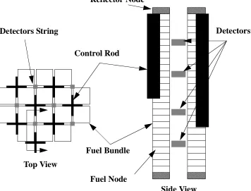
Figure 4.1: Detectors Layout. . . . 75

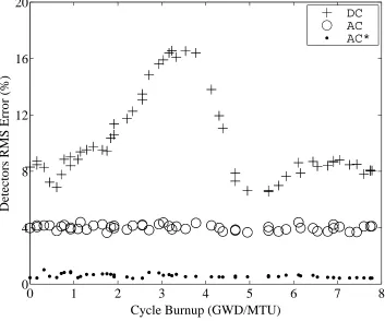
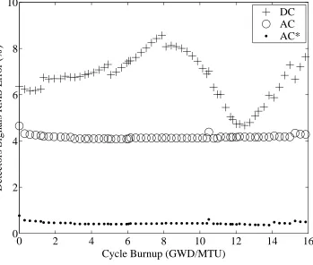
Figure 4.2: Detectors Signals RMS Errors (Case A). . . . 76

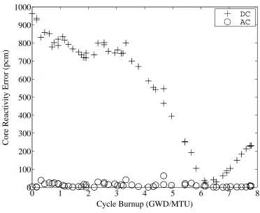
Figure 4.3: Core Reactivity Errors (Case A). . . . 77

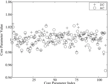
Figure 4.4: A Priori and A Posteriori Core Parameters Values (Case A). . . . 78

Figure 4.5: Detectors Signals RMS Errors (High Void) (Case A). . . . 79

Figure 4.6: Core Reactivity Errors (High Void) (Case A). . . 80

Figure 4.7: Detectors Signals RMS Errors (Low Void) (Case A). . . . 81

Figure 4.8: Core Reactivity Errors (Low Void) (Case A). . . . 82

Figure 4.9: Detectors Signals RMS Errors (Future Predictions) (Case A). . . . 83

Figure 4.10: Core Reactivity Errors (Future Predictions) (Case A). . . . 84

Figure 4.11: Detectors Signals RMS Errors (Case B). . . . 85

Figure 4.12: Core Reactivity Errors (Case B). . . . 86

Figure 4.13: Axial Core Power RMS Errors (Case B). . . 87

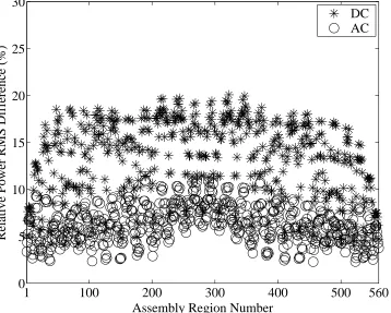
Figure 4.14: Assemblies Powers RMS Errors Towards Beginning of Cycle (Case B). . 88

Figure 4.15: Assemblies Powers RMS Errors During Mid of Cycle (Case B). . . . 89

Figure 4.16: Assemblies Powers RMS Errors Towards End of Cycle (Case B). . . . 90

Figure 4.17: Singular Values of The Covariance Matrix of The Multi-group Library . . 91

Figure 4.18: GE 12 Lattice Design Configuration. . . 92

viii Figure 4.21: Axial Core Power RMS Differences

Between FORMOSA-B and VC_u (Case C). . . 95 Figure 4.22: Assemblies Powers RMS Differences Towards Beginning of Cycle

Between FORMOSA-B and VC_u (Case C). . . 96 Figure 4.23: Assemblies Powers RMS Differences During Mid of Cycle

Between FORMOSA-B and VC_u (Case C). . . 97 Figure 4.24: Assemblies Powers RMS Differences Towards End of Cycle

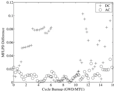
Between FORMOSA-B and VC_u (Case C). . . 98 Figure 4.25: MFLPD Differences

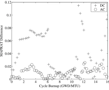
Between FORMOSA-B and VC_u (Case C). . . 99 Figure 4.26: MAPRAT Differences

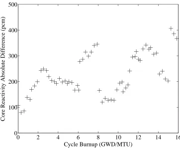
Between FORMOSA-B and VC_u (Case C). . . 100 Figure 4.27: Core Reactivity Differences

Between Reference and Random LP-CRP Pairings as Evaluated by VC_u (Case C). . . 101 Figure 4.28: Axial Core Power RMS Differences

Between Reference and Random LP-CRP Pairings as Evaluated by VC_u (Case C). . . 102 Figure 4.29: Assemblies Powers RMS Differences Towards Beginning of Cycle

ix

Between Reference and Random LP-CRP Pairings as Evaluated by VC_u (Case C). . . 104 Figure 4.31: Assemblies Powers RMS Differences Towards End of Cycle

Between Reference and Random LP-CRP Pairings as Evaluated by VC_u (Case C). . . 105 Figure 4.32: Core Reactivity Differences

Between FORMOSA-B and VC_u for Random LP-CRP Pairing

(Case C). . . 106 Figure 4.33: Axial Core Power RMS Differences

Between FORMOSA-B and VCu for Random LP-CRP Pairing

(Case C). . . 107 Figure 4.34: Assemblies Powers RMS Differences Towards Beginning of Cycle

Between FORMOSA-B and VC_u for Random LP-CRP Pairing

(Case C). . . 108 Figure 4.35: Assemblies Powers RMS Differences Towards Mid of Cycle

Between FORMOSA-B and VC_u for Random LP-CRP Pairing

(Case C). . . 109 Figure 4.36: Assemblies Powers RMS Differences Towards End of Cycle

Between FORMOSA-B and VC_u for Random LP-CRP Pairing

x Figure 4.38: Axial Core Power RMS Differences

Between FORMOSA-B and VC_u (Case D1). . . 112 Figure 4.39: Assemblies Powers RMS Differences Towards Beginning of Cycle

Between FORMOSA-B and VC_u (Case D1). . . 113 Figure 4.40: Assemblies Powers RMS Differences During Mid of Cycle

Between FORMOSA-B and VC_u (Case D1). . . 114 Figure 4.41: Assemblies Powers RMS Differences Towards End of Cycle

Between FORMOSA-B and VC_u (Case D1). . . 115 Figure 4.42: MFLPD Difference

Between FORMOSA-B and VC_u (Case D1). . . 116 Figure 4.43: MAPRAT Differences

Between FORMOSA-B and VC_u (Case D1). . . 117 Figure 4.44: Core Reactivity Differences

Between FORMOSA-B and VC_u (Case D2). . . 118 Figure 4.45: Axial Core Power RMS Differences

Between FORMOSA-B and VC_u (Case D2). . . 119 Figure 4.46: Assemblies Powers RMS Differences Towards Beginning of Cycle

Between FORMOSA-B and VC_u (Case D2). . . 120 Figure 4.47: Assemblies Powers RMS Differences During Mid of Cycle

xi Figure 4.49: MFLPD Difference

Between FORMOSA-B and VC_u (Case D2). . . 123 Figure 4.50: MAPRAT Differences

Between FORMOSA-B and VC_u (Case D2). . . 124 Figure 4.51: Core Reactivity Uncertainty (Case E). . . . 125 Figure 4.52: Fuel Assemblies Axial Power Distribution Uncertainty

Towards Beginning of Cycle (Case E).. . . 126 Figure 4.53: Fuel Assemblies Axial Power Distribution Uncertainty

During Mid of Cycle (Case E). . . 127 Figure 4.54: Axial Core Power Distribution Uncertainty

Towards End of Cycle (Case E).. . . 128 Figure 4.55: Axial Core Power Distribution Uncertainty

Towards Beginning of Cycle (Case E).. . . 129 Figure 4.56: Axial Core Power Distribution Uncertainty

During Mid of Cycle (Case E). . . 130 Figure 4.57: Axial Core Power Distribution Uncertainty

Towards End of Cycle (Case E).. . . 131 Figure 4.58: Radial Core Power Distribution Uncertainty

Towards Beginning of Cycle (Case E).. . . 132 Figure 4.59: Radial Core Power Distribution Uncertainty

xii

xiii

Acronyms:

ACS Adaptive Core Simulation

AC Adapted Design Basis Core Simulator BOC Beginning Of Cycle

BWR Boiling Water Reactor CRH Control Rod History

CRD Control RoD Insertion Branch Case DC Design Basis Core Simulator DIT Discrete Inverse Theory DAT Data Adjustment Techniques ESM Efficient Subspace Methods EOC End Of Cycle

FP Fission Products Branch Case HFP Hot Full Power

HV High Void

LCBD Lattice-Configuration/Base-Depletion LPRM Local Power Range Monitors

LV Low Void

xiv

PWR Pressurized Water Reactor RMS Root Mean Square

REF REFerence or Base Depletion Case RV Rated Values

STU Short-Tonnes-U, STU=1.1023113 MTU SVD Singular Value Decomposition

TIP Traveling Incore Probe

xv Void-quality concentration parameter. Void-quality terminal velocity parameter. Density of the vapor phase.

Density of the liquid phase. Void fraction.

x Flow quality.

G Coolant mass flux.

Surface tension, microscopic cross-section or standard deviation. Void-quality drift velocity parameter.

g Gravitational acceleration constant.

k_eff Core criticality eigenvalue.

Variables’ Notations:

Scalar quantity. Nonlinear Operator.

Vector quantity. Matrix Operator.

C₀ k₃ ρ_g ρ_g α

σ

V_gj

*

* .( )

*

1. Introduction

1.1. Importance to Advanced and Current Reactors

The accurate prediction of core behaviour is a fundamental requirement to the design and operation of any nuclear reactor system. That is achieved through the utilization of high fidelity core simulators. Core simulators can be utilized in either an on-line or off-line mode. In an online mode, they provide support for the successful control and protection of the reactor. Control systems are required to determine the optimum trajectory in moving the reactor from the current state to a final desired state with all operational and safety limits satisfied. Protection systems are required to be capable of determining current and near-term reactor states for a range of reactor conditions to advise reactor operators, or to automatically activate safety systems to help take the appropriate actions to avoid and/or mitigate any accident scenarios. In an off-line mode, core simulators are as important during the design as well as operational phases of the plant to determine the optimum operating core conditions, e.g. fuel loading pattern, control rod programming, etc., over the operating horizon of a nuclear power plant, i.e. over multiple depletion cycles. They are also utilized to interpret experimental results.

other hand, any reduction in these uncertainties will beneficially impact different aspects of reactor economy such as reducing fuel and/or operating cost or even initial capital investment for a new plant. By way of a few examples[2]: 1) By accurately calculating thermal limits, one can reduce thermal margins, and be able to operate the reactor at higher power densities which is economically more favorable (energy cost reduction). That translates into smaller sized cores for new reactors (reduction in capital investment). 2) With more accurate calculations of core reactivity for various states, one may be able to reduce the number of control rods (reduction in capital investment), or reduce the U235 enrichment margin required in the fresh fuel for the core to reach the desired cycle life at the desired rated power (reduction in fuel cost).

however, are referred to as core attributes, such as local power peaking and thermal margins, which are important for core design and operation. Core attributes are not directly measured, however special techniques exist to relate them to core observables. These techniques include diffusion theory-type calculations, response surface methodologies, and ordinary least-squares fitting procedures that we believe are questionable, hence we choose not to employ core attributes in the adaption[3]-[4]. Now, a robust adaption must be able to predict the important core attributes that are not utilized by the adaptive algorithm. Further, a robust adaption must predict the measured core observables for core conditions that differ from those at which adaption is completed, e.g. the measured observables recorded at future times and/or different core power levels.

Adaptive simulation can also be useful in establishing a basis for deciding where future experimental efforts should be focused to decrease core attributes uncertainties. That can be achieved by contrasting the core simulators adjusted input data values versus their current known values, along with knowledge of the impact their adjusted values will have on different core attributes, the costs associated with uncertainties on these core attributes, and the costs of experiments to reduce core attributes uncertainties.

Our current research interest is focused on enhancing the fidelity of BWR core simulators, since their prediction accuracy is inferior to PWRs, providing marginally acceptable agreement between measured and predicted core attributes. This implies that BWRs would benefit from utilizing an adaptive simulation tool.

1.2. Proposed Adaptive Techniques

Our proposed adaptive techniques utilize a group of mathematical techniques that address the problem of given a current core simulator model and the associated input data, how should the values of the multitudes of input data be adjusted in a statistically consistent manner without changing the core simulator model1 to improve agreement with core observables in a robust fashion. The object is to obtain the best possible agreement utilizing our current modeling capability[5]. This is usually referred to as an inverse problem, which is difficult to solve due to its ill-posedness nature. Major advances have been made by Mathematicians to overcome the ill-posedness nature of such problems. One goal for the research reported upon here is to develop expertise in this area, to which the nuclear power community has not participated to any great extent over the last two decades. Exceptions include some work conducted on solving the inverse radiation transport problems utilizing neural networks[6]. Techniques based on neural networks are fundamentally different from our development since the neurons (basic elements in a neural network) response functions then employed to represent core simulators are not related to the conventional core simulators physics models.

calculating a least-squares solution to a linear systems of equations involving million of unknowns.

1.3. Thesis Organization

Even though the subject of the thesis is very mathematical in nature, we choose to keep the discussion, throughout the thesis, as intuitive as possible rather than rendering it to be of a mere abstract nature. We prefer the intuitive approach in order to help construct an integrated framework, or the big picture, especially when exploring a new research area. However, we intend to provide some preliminaries to set the stage for the discussion; but we will refrain from reproducing any mathematical results that can be found elsewhere. The focus will only be on the ESM results that are novel to our work. However, for the sake of a complete discussion, a list of references will be suggested for the more interested reader. In the appendix, we develop the mathematical foundations and theory behind ESM. In doing so, we choose not to cast the discussion into the mold of nuclear reactor core calculations, however we present a generalized framework that other scientists, engineers, and applied mathematicians can easily relate to, understand, and eventually develop to suit their specific needs.

1.4. Overview of Nuclear Reactor Core Calculations

Heat energy is generated after a neutron collides with a fissionable material causing it to split into several lighter elements referred to as fission fragments. In this process, the energy released in fission is transformed into kinetic energy of the formed fission products. During slowing down, fission products quickly lose their energy to the media in the form of heat energy. Fission is not the only event that is responsible for energy release. For example, a neutron may be absorbed by the target nucleus followed by the emission of a gamma ray that eventually deposits its energy in the media in the form of heat as well. More details on this process may be found in any of numerous textbooks written on nuclear physics[9].

The basic underlying physics governing neutron interaction with matter is described by cross-sections data. Cross-sections are evaluated experimentally; they characterize the interaction probability of a neutron travelling at a certain speed in a certain direction with matter, e.g. target nucleus. Upon interaction, a neutron may disappear, i.e. absorbed, or change its speed and direction of travel, i.e. scattered. Cross-sections data are tabulated as a continuous function of incident neutron energy, target nucleus type, and reaction type and are referred to as point cross-sections. The Evaluated Nuclear Data Files ENDF/B is one source for the point cross-sections data in the United States[10].

cross-section variation in an energy group can be adequately represented by an single average value, referred to as the group cross-section. A typical number of groups used in thermal reactor core calculations is 20-50 energy groups. Mathematically, the neutron interaction with media using the multi-group approach is modeled as a transport phenomena. The transport equation is a nonlinear integro-differential equation1. The solution of this equation is referred to as the neutron angular flux - a vector quantity that is equal in magnitude to the product of neutron density and speed and points in the neutrons direction of travel. Angular flux is a function of energy group, direction of travel, space and time. Being simple to write down, the multi-group equations are very hard to solve for the whole reactor core with current computing resources. A typical BWR core contains about 400-800 fuel assemblies. Each assembly contains about 5 different axial fuel zones. Each zone is a square array of approximately 90 fuel pins with 10 different compositions. Capturing this level of details for the whole core is likely not feasible in the near future from either a computational or a storage consideration. Luckily, core designers are only interested in some integral properties of the neutrons distribution. These integral properties are often referred to as core attributes, such as power distribution and core reactivity. Consequently, more simplified models, often referred to as core simulators, are devised to directly calculate the desired core attributes. These models are based on coarse spatial mesh and few energy groups. The input data to core simulators, including few-group cross-sections, are prepared by another set of codes, referred to as the preprocessor codes. Preprocessor codes capture the details that are left out by core

simulators models; their models are based on fine spatial mesh and many energy groups. The next few sections briefly overview the preprocessor codes and core simulators models.

1.5. Overview of Preprocessor Codes

Preprocessor codes are a cascade of computer codes that prepare basic reactor physics data available in the ENDF/B format and thermal-hydraulics input data into a format that is consistent with core simulators physics models. These codes include multi-group generation codes that collapse the ENDF/B point-wise continuous energy representation of cross-sections into a multi-group format, e.g. 238, 44, or 27 energy groups. Preprocessor codes also include lattice physics codes which model each spatial zone, i.e. lattice, in a fuel assembly in detail and calculate homogenized (constant for the whole zone) and collapsed (2 or 3 energy groups) few-group cross-sections. Finally, any other buffer code that may be utilized for special purposes, e.g. for cross-sections resonance treatment, is considered a part of the preprocessor codes cascade. In our work, the input data to the core simulator code employed were prepared by the NJOY code for generating multi-group cross-sections library into a 44 energy group format[11]. The multi-group library is then input to the CASMO code for performing lattice physics calculation to generate the few-group cross-sections data into a 2 energy group format[12].

reference cross-sections library. The perturbations are based on the available ENDF/B uncertainty information. The preprocessor codes are then utilized to calculate a perturbed set of few-group cross-sections data. The results are assembled as will be shown in chapter III to calculate the few-group cross-sections covariance matrix. It is evident that a complete set of preprocessor codes should be available to carry out this task. Unfortunately, the CASMO code employed to generate the reference few-group cross-sections data is a commercial proprietary code. In search of an alternative, we have utilized another set of preprocessor developmental codes supplied by Oak Ridge National Laboratory (ORNL) - the AMPX-TRITON[13]-[14] code system is employed to replace the NJOY-CASMO system with regard to propagating ENDF/B uncertainty information. The reference values for few-group cross-sections however are still evaluated using the NJOY-CASMO system.

1.6. Overview of Core Simulators

Core simulators employ both reactor physics and thermal-hydraulics models to account for the nonlinear feedback mechanisms through few-group cross-sections. Typically, reactor physics behavior is modeled employing few-group neutron diffusion theory, hydraulics behaviour is modeled employing some 1-D approximate form of the Navier-Stokes equations, e.g. drift flux model, and the thermal behavior is modeled using some approximate thermal model, e.g. functionalizing fuel temperature as a function of linear power density.

determined by lattice physics codes that model aspects of the core physics in more details than core simulators models, e.g. the few-group homogenized cross-sections generated by CASMO or TRITON. Likewise, portions of the thermal-hydraulics input data are determined employing more detailed thermal-hydraulics models, e.g. fuel temperature models. So, in general, the input data include any data directly passed to the core simulator or indirectly through any preprocessor code. A typical size of the input data to a core simulator is of the order of 105-106 data values.

Core observables include the readings of in-core detectors, e.g. for BWRs LPRMs and TIPs which are usually positioned throughout the core between flow channels which do not have control rods. Since core simulators are usually based on a steady state model and measured observables are normally taken at steady state conditions, core reactivity could also serve as a basis for adaption, i.e. at all times for real plant data. Ultimately, one would use the just noted core observables to adjust current core simulators predictions to match actual plant data. However, in the course of developing and assessing adaptive simulation techniques, another set of core observables have been utilized. In particular when adjusting a core simulator to agree with another core simulator predictions in a virtual sense, i.e. one of the two core simulators is assumed to represent actual plant data. In this case, node-wise1 powers may be utilized as core observables. This process is elaborated on in chapter II, where the virtual approach is discussed in details. In our work, a typical number for core observables is of the order of 104-106 data values.

1. Each fuel assembly is divided into a number of axial fuel nodes as required by numerical discretiza-tion techniques (24 axial nodes is typical for BWR calculadiscretiza-tions). Node-wise powers refers to the val-ues of generated power in each axial node throughout the core.

The core simulator employed in our work is called FORMOSA-B. It is a proprietary code developed by the NC State Electric Power Research Center (EPRC).

1.7. Sources of Simulation Errors

Core simulators introduce errors in the predicted core observables, including core attributes, due to input data errors and computational errors, i.e. modeling errors. Input data, whether they are experimentally measured or theoretically calculated, contain uncertainties associated with their evaluation which are described by covariance values reported as part of the data evaluation process. Modeling errors occur due to different reasons: 1) The common practice in modeling is to avoid sophistication by introducing approximations in the mathematical description to simplify the treatment. This results in the introduction of errors in the calculations, e.g. diffusion versus transport theory calculations for the whole core. 2) Inadequacies in the mathematical model utilized for simulating the core, e.g. failure to present all aspects of the physics governing the core behaviour. 3) Numerical solution techniques approximations, e.g. spatial domain discretization.

1.8. Adaptive Core Simulation

Computational methods and input data uncertainties have always been the sources of the limitation of nuclear calculations. In some instances, the computational uncertainties dominate the sources of discrepancies between measurements and predictions. However, over the last few decades, computational methods have reached a stage of maturity in their sophistication and applicability. Computational power has also increased considerably enabling the solution of bigger problems in relatively shorter computer execution times. With the current status of models sophistication and huge experience obtained from power plants operations, we believe that more attention should be directed towards input data errors. This can be realized in practice by utilizing the large volume of observables data generated from operating nuclear power plants to effectively reduce the disagreement between the measured and predicted core observables, and if done correctly, the accuracy of predicted core attributes. It is surprising enough to know that to date there has been no systematic attempt to use this vast quantity of operating observables data to improve simulation accuracy with regard to core simulators predictions. Clearly there are issues related to quality of data, e.g. detector failure or drift, or assumed core equilibrium state, that in practice need to be addressed. For now, we defer treating such issues to limit scope. In this regard, we recognize that much capability has been developed in regard to interpreting validity of detectors signals.

1.8.1 Proposed Adaptive Simulation Techniques

adjusting the model in order to reduce the disagreement between the measured and predicted observables. The sources for the disagreement are assumed to be either due to noise in the measured observables or simulation errors which, as described before, consist of modeling and input data errors. Accordingly, it will be assumed that the dominant sources of core simulation errors in predicted core observables, including core attributes, originate due to errors in the input data to the preprocessor codes and preprocessor codes independent input data to the core simulator. That implies that input data will be adjusted to improve the agreement between predicted and measured core observables, even though components of the sources of disagreement are due to both input data and modeling errors. This assumption is likely valid and also necessary in order to avoid the issue of simultaneous adaption of the core simulator models, since the combined adaption problem of core simulator input data and models is beyond current and foreseeable capabilities. However, a justification for that assumption has to be investigated in this study by checking the fidelity and robustness of the adaption.

1.8.2 Adaptive Simulation Concerns

There are different issues and concerns that need to be analyzed when adjusting input data in this fashion[15]. How well will the adjusted data perform at different core conditions and how consistent are they with the unadjusted data? If unconstrained by the data uncertainty, would one obtain the same results utilizing two different data sets and the same measured observables to adapt the core simulator? This type of analysis can also help answer some other questions such as: 1) How well do the existing input data predict the core attributes of interest with the current modeling capabilities? 2) How sensitive are certain core attributes to changes in the input data? 3) How does one identify the sources/causes of discrepancies between the core simulators predicted and measured core observables? Answering question (3) will provide direction to those areas of uncertainty where more detailed experimental programs are required to decrease core attributes uncertainties.

1.8.3 Differences to Previous Development

First, instead of using small scale experiments to simulate the operation of the real reactor, one can use the full scale experiment, i.e. real core, as one’s integral experiment. This is advantageous when considering the huge amount of core follow data from our operating experience with current power plants. However, the interpretation of these data is much more complex than the “clean” integral experiments, since the quality of the data is uneven and nonlinear feedback effects are present. For integral experiments, the quality of the data is considered to be the same, since there are no depletion effects and no nonlinear thermal-hydraulic feedback effects. In addition, for power plants transient phenomena might be occurring at anytime yet a steady state core model is employed, and instrumentations may not be properly calibrated or failed.

same input data adjustments. However, for ill-posed problems, DAT are subject to the same problems of ordinary least-squares adjustment techniques, e.g. the unphysical adjustments of insensitive input data.

changes in core observables would be as big as . Evidently, storing such a matrix presents a challenge by itself.

Fourth, the last feature that distinguishes our proposed adaptive techniques from earlier data adjustment techniques is the capability of confining the adjusted input data to be within their a priori uncertainty limits. That requires the availability of the uncertainty information of core simulators input data, i.e. propagated from ENDF/B libraries to core simulators level. This is not a trivial task to do and requires another sensitivity study that is even far more demanding than the one required for core simulators adaption. That is clear when one considers how large the amount of cross-section data contained in ENDF/B libraries are. Also note that, even if the core simulators input data uncertainties are available, that would be a huge storage burden. This follows since uncertainty information is often characterized by a covariance matrix which, in our case, is of the order of . Again, it is impractical to store such a matrix.

One concludes that the associated computational and storage burdens pose significant challenges for the proposed adaptive techniques. One of the main goals of this thesis is to develop an effective approach that will reduce the computational and storage cost associated with the core adaption problem to an acceptable level. This is to be achieved without compromising the fidelity of the adaption or violating the statistical consistency of the adjusted input data with their a priori values. Our effective approach is based on a set of mathematically efficient methods employed to approximate the action of very large, dense matrix operators. We denote these methods by the Efficient Subspace Methods (ESM). The mathematical development of ESM is an integral part of this thesis.

106×104

1.8.4 Current Adaptive Techniques

2. Virtual Approach

2.1. Overview of Virtual Approach

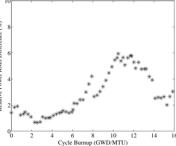
core reactivity and in-core detectors signals RMS errors. The created discrepancies are of the same magnitude as the actual discrepancies found between real plant data and existing core simulators predictions1. In this approach, the simulated in-core instrumentations serve as core observables that are used for adapting the DC.

In the second approach, the DC is represented by a core simulator different from the one utilized to generate the VC data. The two core simulators, the VC and the DC, are selected so as to have fundamental differences in their modeling and input data functionalization. This approach will help demonstrate how robust adaptive techniques are when the sources of errors are not known, which is the real situation. Also of a recent interest to our other research areas, this approach has the potential benefit of allowing us to adapt the core simulator model in our in-core fuel management optimization code, FORMOSA-B, to better agree with a utility’s or fuel vendor’s design basis core simulator. Reducing the inconsistencies between the two core simulators will provide higher confidence that FORMOSA-B determined optimized loading pattern-control rod patterns (LP-CRP) pairings are also found optimum and feasible when re-evaluated using their design basis core simulator. In this approach, we elect node-wise powers to serve as core observables. Obviously, more applications can be realized in practice by having an adaptive tool that can enhance the agreement between two different simulation codes systems.

1. A representative value for the core reactivity prediction error is around pcm, and the

RMS error for relative detectors signals is about 6%.

2.2. Advantages of Virtual Approach Utilization

In contrast to utilizing operating power plant observables, the virtual core approach has several attractive properties in regard to developing an adaptive core simulator methodology, such as the following: 1) Knowing exactly the sources of errors in the method, input data and observables. 2) Providing a basis to study the effects of the parametrization of core simulator model on the fidelity and/or robustness of the adaptive simulator. 3) Having not to contend with the complexities of core simulator and preprocessor introduced methods errors. 4) Being able to evaluate the prediction accuracies of non-observables, i.e. thermal margins, obtained from pre- and post-adaption. 5) Developing a capability to reduce inconsistencies between two different code systems.

2.3. Core Parameterization

This section presents a description of the core models and input data that are adapted in our proposed virtual approach. Core parameterization is the process in which modeling and input data errors are fully characterized by a pre-selected set of parameters. Core parameters are selected so as to functionalize the errors in terms of different core conditions, e.g. fuel exposure, instantaneous and history voiding, etc. Adjusting core parameters would be considered equivalent to adapting the simulation. Hence, care is required in the selection of these parameters since improper choice would be reflected in poorer fidelity and/or robustness of the adapted core simulator.

not directly adjust input data but rather a selected set of core parameters, i.e. a function of input data, the uncertainty information about core parameters ought to be available a priori. This is a straightforward task once the input data uncertainty information is available, it can easily be propagated to uncertainties in the selected core parameters. More details on this process will be revealed in chapter III.

2.3.1 Modeling Errors

Modeling errors have been included in the DC by recognizing that the modeling of voids in a BWR core has a large impact on the prediction of different core attributes such as the power distribution and reactivity. Based on that fact, the void-quality correlation was perturbed in the DC. The void-quality1 relationship is given by the form identified by Zuber-Findlay [41]:

. (1)

The DC utilized the Zuber-Findlay void-quality correlation in which two variables, the concentration parameter ( ) and terminal velocity parameter ( ), were assumed spatially independent throughout the core and given by their best known values, i.e. and . Core parameterization adapted these two variables according to the following relations2:

. (2)

1. Refer to Moore’s Ph.D. thesis for more details [40], all symbols have their standard interpretation. 2. The adjusted input data are tilded, and the various factors are the selected core parameters to be

adjusted with superscripts and/or subscripts identifying the particular input data with which they are associated.

α x

C₀ x ρg ρ_l

--- 1( –x)

+ ρgk3

G

--- (ρl–ρg)σg

ρ_l2

---4

+

---=

C₀ k₃

C₀ = 1.13

k₃ = 1.41

p

C˜0 p

c0

C₀; k˜3 p

k3 k₃

The multipliers and represent the selected thermal-hydraulics core parameters to be determined by the adaptive techniques. The VC, however, utilized the Lellouche-Zolotar EPRI methodology[42] to determine and , which can be thought of as using spatially dependent and . Functionalization of the void-quality correlation in these two different manners will help us investigate how well the adaptive technique will perform when the functionalization of the data is not consistent with reality, i.e. employing core observables predicted using the Zuber-Findlay void-quality correlation to attempt to match those predicted using the Lellouche-Zolotar void-quality correlation. Also, this functionalization will demonstrate how adaptive techniques can account separately for the combined sources of errors due to inconsistent modeling and input data errors.

2.3.2 Input Data Errors

The second source of errors included in the virtual approach is due to input data errors. The thermal-hydraulics data in the current study consists of only the and , coefficients of the Zuber-Findlay void-quality correlation. The reactor physics input data consists of all types of few-group homogenized fast and thermal microscopic cross-sections, i.e. absorption, fission, prompt and energy yields per fission, of all nuclides included explicitly or implicitly in the microscopic depletion model, i.e. actinides, burnable poison isotopes and background pseudo isotopes, of the utilized core simulator. The cross-section representation utilized by FORMOSA-B requires that a number of ‘cases’ be generated at the lattice physics level. Base micro and/or macroscopic cross-sections are obtained from a lattice physics unit assembly depletion at the nominal hot full power (HFP) average core conditions at different vapor void

pc0 pk3

C₀ k₃

C₀ k₃

fractions. From the base cases, branch cases are performed to capture the instantaneous effects of perturbing different core conditions, e.g. fuel temperature, coolant void, and control rod insertion. The cross-section is constructed as the summation of a reference term and a set of correction terms given by:

(3) where the reference term is the first term on the R.H.S. and is a function of fuel exposure, and instantaneous and history void fractions. The remaining terms are correction terms, accounting for control rod history, fuel temperature Doppler broadening effect, fission products poisoning, and instantaneous control rod insertion effect. The reference and the correction terms are constructed using piece-wise cubic splines and quadratic fitting polynomials, which for term k of cross-section type j for nuclide n in fuel color c is given by:

, (4)

where is a state variable describing the dependence of the specific cross-section reference or correction term on different core conditions, i.e. fuel temperature, void fraction, etc., { } are the polynomial coefficients calculated based on the lattice physics data functionalized in terms of the fuel exposure, , and { } are polynomial functions.

Different functionalizations may be employed to characterize input data errors. A study of which functionalization might be of most benefit for BWR adaption represents one of our on-going research tasks. In the interum, however, we apply a simple core

Σ ΣREF ΣCRH ΣTF ΣF P ΣCRD

+ + + +

=

Σn j k c, , ,

Bu

( ) d_in j k c, , , (Bu) y_i( )x

i

∑

=

x

d_in j k c, , ,

parameterization, in which the reference and correction terms are adapted according to the relation:

, (5)

where the multipliers are functionalized in terms of fuel exposure in the following way:

. (6)

The { } represent the reactor physics core parameters to be

determined by the adaptive techniques, and is a scaling factor with exposure units. To simulate input data errors, core parameters are randomly selected from Gaussian distribution based on the available core parameters uncertainty information. The uncertainty information is mathematically described by a symmetric covariance matrix. The diagonal elements of this matrix represent the errors of core parameters (variance units), while the off-diagonal elements quantize the degree of correlation among these errors. Earlier in our development, the core simulators input data uncertainty information was not yet available. Hence, we assumed a diagonal core parameters covariance matrix with equal diagonal entries. Evidently, this is a very crude assumption since errors in the few-group homogenized cross-sections are correlated in general, and hence the off-diagonal entries of the associated covariance matrix are expected to be non-zero. At this time, the preprocessor codes were not yet available and hence one had to resort to this crude assumption in order to continue studying the general potential of adaptive techniques for core physics problems. In this case, the size of the perturbation (1% for all core parameters) is selected such as to give rise to

Σ˜n j k c, , , _{(Bu) p} i n j k c, , ,

Bu

( )d_in j k c, , , (Bu) y_i( )x

i

∑

=

p_in j k c, , ,

p_in j k c, , , (Bu) p_{i 1}n j k c_,, , , (1–p_{i 2}n j k c_,, , , ) Bu Bu˜

--- 

  _{1 p}

i 3, n j k c, , , –

( ) Bu

Bu˜

--- 

 2

+ +

=

p_{i 1}n j k c_,, , , ,pn j k c_{i 2,}, , , ,and p_{i 3}n j k c_,, , ,

3. Mathematical Development

In this chapter, we introduce the mathematical description of the proposed adaptive simulation techniques. The mathematical vehicle is linear algebra theory; ideas like vector spaces, and matrix representations of linear transformations are sufficient to fully characterize the problem. The proposed adaptive simulation techniques can be fully described in terms of optimization techniques by vector space methods. We assume that the reader is rather familiar with basic linear algebra and vector space concepts and notions, such as vectors, matrices, basis, span, space, subspace, orthogonality, etc. In the appendix however, we shed more light on the basic linear algebra operations; this will provide the insight required to introduce our novel Efficient Subspace Methods (ESM)1.

In our discussion, we will first focus on introducing the conventional approach to implementing inverse theory to core adaption problem. The target will be to convey to the reader the inherent computational and storage difficulties that are spawned by the direct application of conventional techniques. We will then introduce the proposed ESM algorithms, discuss their implementation and leave the supporting mathematical proofs to the Appendix. Since the scope of ESM is beyond nuclear reactor calculations; we believe a much wider audience may benefit from the introduced techniques. Therefore, we choose to format the appendix as a stand-alone paper that discusses ESM in a more generalized framework that can suit a wider audience. However, the notations introduced in this chapter with regard to core adaption problem are consistent with those introduced in the appendix, so the thesis reader

should have no difficulty comprehending the appendix applicability to the core adaption problem.

3.1. Conventional Development

Let the core design basis simulator model be represented by the following vector nonlinear equation:

, (3-1)

where is a vector of dimension whose components are the selected core parameters, i.e. the various factors1, and the subscript ‘ ’ distinguishes the vector that represents the a priori knowledge about core parameters. The is a vector of dimension whose components represent the predicted (calculated) core observables, i.e. core reactivity, in-core detectors readings, and/or node-wise powers.

Let the preprocessor codes and the selected core parameterization be represented by the following nonlinear equation:

, (3-2)

where is a vector of dimension whose components are the basic input data, including reactor physics data, thermal-hydraulic data, and any other input data to the preprocessor codes. Note that, in this context, denotes a cascade of codes that, by way of example, take as input the multi-group cross sections data and produces at an intermediate stage the few-group cross-sections data, i.e. lattice physics codes. Then, based on the selected core

1. from chapter II.

Ω₀ = Θ Γ( )₀

Γ₀ n

p 0

Γ₀ = [pc0 pk3 ... p_in j k c, , , ... ]

Ω₀ m

Γ₀ = Π ϒ( )₀

ϒ₀ l

parameterization, the few-group cross-sections data and the thermal hydraulic data are converted into their respective core parameters. To avoid introducing cumbersome notations, we denote by the preprocessor codes, even though it contains our proposed core parameterization step at its back end.

The objective of the proposed adaptive techniques is to adjust core parameters such as to decrease the discrepancies between the measured and predicted core observables. To ensure a robust adaption, the adjusted core parameters are constrained by their a priori uncertainty information. This information is currently available at the input level to the lattice physics code, i.e. the uncertainties of the multi-group cross-sections are available1. Hence an integral goal for this thesis is to devise a methodology to propagate uncertainties in the multi-group data to uncertainties in core parameters, or in general to uncertainties in the few-group cross-sections data.

Now, let’s introduce the mathematical algorithm employed by adaptive techniques to adjust core parameters. Core parameters are selected so as to satisfy the following constrained minimization problem:

subject to (3-3)

1. Recall from the introduction chapter, we use the AMPX-TRITON preprocessor codes to propagate uncertainty information. Uncertainty information of the basic input data are originally available in the point-wise ENDF/B library format. The AMPX code system is however capable of propagating uncertainty information from ENDF/B library formats to the multi-group library format. Hence, we do not repeat this step and start directly from the multi-group libraries with regard to uncertainty propagation. Hereinafter, any reference to the ‘basic input data’ denotes reactor physics data in the multi-group cross-sections format instead of the ENDF/B library format.

Π

Γˆ min

Γ Λ0 Ω

–

[ ]TC_Λ+[Λ₀–Ω]

{ }

where is a vector of measured core observables, is the observables covariance matrix, and is the core parameters covariance matrix (the superscript denotes the Moore-Penrose pseudo inverse operator). In this formulation, core parameters are selected to minimize the disagreement between the measured and predicted core observables, while still constraining them to a region of the search space, i.e. the ellipsoid defined by the constraint, where they are statistically consistent with their a priori values. The minimizer of Eq (3-3) is referred to as the a posteriori estimate of core parameters. It can be shown that this inequality constrained minimization problem is equivalent to the following penalized unconstrained minimization problem[48]:

(3-4)

subject to , where is called a regularization parameter and is selected such that the constraint in Eq (3-3) is satisfied1. Different regularization approaches offer different ways to determine the optimum values for the regularization parameter , based upon different criteria. For the current work, we performed a parametric study to determine their optimum values experimentally, by “trial and error”, based upon the characteristic ‘L-curve’[49]. The first term in Eq (3-4) is referred to as the misfit term, and the second term is referred to as the regularized term. If the selected regularization parameter approaches zero, the problem reduces to an ordinary least-squares case and the parameters adjustment are mainly determined by the observables; whereas, if the regularization parameter approaches

1. Notice that Eq (3-4) includes two minimizations. This follows since the core parameters ans core observables covariance matrices do not have full ranks in general.

Λ₀ C_Λ

C_Γ +

Γˆ

Γˆ min

Γ˜

Γ˜ min

Γ [Λ0–Ω]

T

C_Λ+[Λ₀–Ω] α+ 2[Γ₀–Γ]TC+_Γ[Γ₀–Γ]

{ }

= =

Ω = Θ Γ( ) α = α ε( )

infinity, the data misfit term is negligible with respect to the regularized term, and the parameters are mainly determined by the a priori information.

Eq (3-4) represents as a nonlinear least-squares unconstrained minimization problem which is usually solved in an iterative fashion, where for each iterate, the nonlinear function to be minimized is approximated by a convex function whose minimum is relatively easier to obtain. Different methods require different information about the convex function to be minimized. In our development, we will consider those methods that require the gradient information only, i.e. the sensitivity coefficients of core observables with respect to core parameters. The reason for this consideration is that we have noticed over the course of this research that the size of the adjustments in core parameters is often small, leading the nonlinear search to converge in a single iteration. Hence we are inclined to utilize the gradient information only and replace Eq (3-1) and Eq (3-2) by their linearized forms, obtained by performing a Taylor series expansion of the later two equations around their respective reference conditions to obtain:

, (3-5)

, (3-6)

where

, (3-7)

. (3-8)

Ω = Ω₀+Θ Γ Γ( – 0)

Γ = Γ0+Π ϒ ϒ( – 0)

Θ

[ ]_{ij Γ}

j

∂ ∂Ω_i

=

Π

[ ]_{ij ϒ}

j

∂ ∂Γ_i

The matrix operators and are referred to as the Jacobian operators associated with the nonlinear models and , respectively. The linearized forms are valid only for small variations of the input data. Therefore, we assume that the adjusted core parameters are close enough to the reference conditions such that the linear approximations given by Eq (3-5) and Eq (3-6) are sufficiently accurate. The a posteriori estimate of core parameters. i.e. the minimizer of Eq (3-3) is given by:

. (3-9)

Let’s now describe what items in Eq (3-4) are available a priori. First, the measured observables are often subjected to noise, measurement drift and calibration errors. We assume that treated a priori are the measurement drift and calibration errors before they enter the calculation in Eq (3-9); however the noise component error persists. Second, the matrix is also available a priori, further we assume that the pseudo-inverse of this matrix may be obtained easily1. Third, the pair ( , ) represent the core parameters and calculated observables, respectively, at the a priori reference conditions. Fourth, the matrix is not available a priori and needs to be calculated based on the uncertainty of the basic input data . Mathematically, may be calculated from:

, (3-10)

where is the covariance matrix of the basic input data which is available a priori. Conventional uncertainty analysis approaches attempt to build the matrix and then evaluate the triple matrix product in Eq (3-10). In this case, it is computationally very expensive to not

1. In our formulation of adaptive techniques, we assume that models are exact and input data

uncertain-ties are the sole source of errors in the predictions. In general, the matrix may be modified to

incorporate modeling uncertainties[26].

Θ Π Θ Π Γˆ Γˆ _Γ 0 Θ T

C_Λ+Θ α+ 2C_Γ+

[ ]†ΘTC_Λ+[Λ₀–Ω₀]

+ =

Λ₀

C_Λ

Γ₀ Ω₀

C_Λ

C_Γ∈Rn×n

ϒ₀ C_Γ

C_Γ = ΠC_ϒΠT C_ϒ

only construct the Jacobian matrix using a conventional sensitivity analysis, but also to perform and/or store the result of the triple matrix product. Similarly, the Jacobian matrix is generally dense and is not available a priori, only a matrix-vector may be calculated as to be later illustrated in Eq (3-12). Finally, examine the minimizer in Eq (3-9); in order to calculate one needs to evaluate two inversions of two very large square matrices with size equal to the number of core parameters, i.e. . Again, this is a prohibitive burden from either a computational or storage standpoints.

Now, let us discuss how conventional sensitivity analysis constructs a Jacobian operator. To build a Jacobian matrix operator (say ), one needs to calculate n directional sensitivity profiles corresponding to the n core parameters of interest. A ‘direction’ refers to a certain perturbation of core parameters from the reference conditions, a total of n independent directions required to span the entire core parameters space. These directions are often chosen to coincide with the standard directions, i.e. perturb only one core parameter at a time. Mathematically, that can be represented as follows: the jth core parameter is incremented by a differential amount and the corresponding jth column of the Jacobian matrix is then calculated according to the formula:

, (3-11)

where is the jth standard basis vector, i.e. that has all its components equal to zero except the jth one is equal to one. This approach is referred to as numerical differentiation or

brute-Π

Θ∈Rm×n

Γˆ

n×n

Θ

δΓ_j

Θ

[ ]_*j [Θ Γ( 0+δΓjej) Θ Γ– ( )0 ]

δΓ_j

---=

force technique. Notice that , the number of core parameters, is too large to render this approach practical.

In the following discussion, we will repeatedly refer to matrix-vector products involving Jacobian operators (say ) of the form: , where is a perturbation in core parameters from the reference conditions , and is the corresponding change in the calculated core observables. The action of the former matrix-vector product may be evaluated by running the nonlinear model twice in the following manner:

. (3-12)

3.2. Efficient Subspace Methods

It is evident from the previous discussion that the main challenge for this research is to devise computationally efficient algorithms to approximate the action of very large and dense matrices1. One of the key contributions of this thesis is to develop the mathematical theory for Efficient Subspace Methods (ESM) and propose algorithms for application with adaptive simulation techniques. They key concept of ESM lies in finding low rank approximations to large and dense matrices which are rank-deficient. This approach has been suggested in the past and is often referred to as Low Rank Approximation or Model Reduction Techniques. Researchers have recognized the significant reduction in computational and storage burdens that may be realized in practice by finding low rank approximations to large matrices. This area has become very popular especially among the computer science researchers in tandem

1. An dense matrix is typical in our applications. This matrix requires approximately 4000

Gigabyte of storage with single precision numbers. Now, consider matrix operations such as

matrix-matrix product, or matrix-matrix inversion will require to say the least operations.

n

Θ δΩ = ΘδΓ ∂Γ

Γ0 δΩ

δΩ = ΘδΓ = Θ Γ( ₀+δΓ) Θ Γ– ( )₀

106×106

with applications such as machine learning and information retrieval techniques[43]. A variety of algorithms have been proposed for different classes of matrices, e.g. moderate size matrices, sparse matrices, block matrices, etc. Most of these algorithms however start running the risk of exceeding practical computational and storage limits when the size of matrices considered becomes too large[44]-[45]. For very large matrices, another class of algorithms have been proposed that randomly sample matrix elements in an attempt to build an appropriate low rank approximation[46]-[47]. These methods however require accessing individual elements of the matrix, e.g. sampling individual rows or columns. This sampling is assumed done without extra computational effort. This feature, however, is not feasible in our case, since the matrices we are interested in are mostly Jacobian operators of nonlinear functions and hence only the effect of a matrix-vector product may be calculated. Therefore, for example, one has to run the forward nonlinear model every time a column is called for by these algorithms. Further, sampling columns or rows in this fashion cannot be justified physically. This follows, since each column represents the sensitivity information of all observables with respect to a certain core parameter. And, each row represents the sensitivity information of a certain observable with respect to all parameters. In this regard, sampling columns or rows is equivalent to limiting sensitivity analysis to only a subset of the parameters and observables, respectively which we are trying to avoid. Finally, these algorithms require calculating matrix-vector products a number of times of the order of the dimensions of the matrix. Again, in our case, that will result in running the nonlinear models too many times to be of any practical value.

than both dimensions of the matrix. Note that the rank of the matrix is not known a priori, it is however determined as a part of the ESM algorithm.

3.2.1 ESM-based Sensitivity Analysis

In the following discussion, we consider the matrix that represents the Jacobian operator associated with the core simulator nonlinear model that relates core observables and core parameters as described by Eq (3-5)1:

Let and . Further, the elements of the matrix are not available, only the matrix-vector product may be evaluated by running the nonlinear model twice, i.e.

, (3-13)

Recall from the previous section, to numerically reconstruct the matrix one needs to run Eq (3-13) times, where for the jth run, one replaces .

Let’s now discuss how ESM builds a low rank approximation to the matrix . The calculation of low rank approximations rests on one fundamental theorem in linear algebra -The Orthogonal Decomposition -Theorem. This theorem states that for any matrix , the following is true:

and , (3-14)

1. The same discussion applies to the preprocessor codes , and the covariance matrices and ;

the discussion however will be limited to avoid redundancy, with reference to the other matrices

made whenever necessary.

Θ

Θ m

n

Π C_ϒ C_Γ

Θ

x_Γ = Γ Γ– ₀ y_Ω = Ω Ω– ₀ Θ

Θ

Ω Ω– ₀ = y_Ω = Θx_Γ = Θ Γ( ) Θ Γ– ( )₀

Θ

n Γ = Γ₀+e_j

Θ

Θ∈Rm×n

where “R( )” and “N( )” refer to the range and null spaces of a matrix, respectively. Put differently, the matrix orthogonally decomposes the core observables and the core parameters spaces each into two complementary orthogonal subspaces:

and . (3-15)

The sizes of these spaces is related to the rank of the matrix according to:

, (3-16)

where “dim( )” refers to the dimension of a space. The distinction between these four subspaces is important in order to gain insight into the action of the matrix operator either in a forward or transposed mode1. Now consider the linearized form of the nonlinear model:

, (3-17)

where and . Eq (3-17) may be re-written utilizing the decomposition in Eq (3-15) as follows:

, and , (3-18)

where , , and . Eq (3-18) implies that any change in core

parameters that belong to does not change core observables. Put differently, only

changes in core parameters that belong to can lead to changes in core observables.

1. In the appendix we elaborate on the similarities between the forward/adjoint notions for a nonlinear model and their equivalent linearized models as represented by the forward/pseudo-inverse matrix operators.

. .

Θ Rm

Rn

Rm = R( )Θ ⊕N(ΘT) Rn = R(ΘT)⊕N( )Θ

r_Θ Θ

r_Θ = dim R( ( )Θ ) = dim R( (ΘT)) = n–dim N( ( )Θ ) = m–dim N( (ΘT))

.

y_Ω = Θx_Γ

x_Γ∈Rn y_Ω∈Rm

y_Ω = Θx_Γ = Θ(x_Γ|| +x_Γ⊥) = Θx_Γ|| Θx_Γ⊥ = 0

x_Γ|| ∈R(ΘT) x⊥_Γ∈N( )Θ y_Ω∈R( )Θ

N( )Θ

Notice that the dimension of the subspace is , implying that only up to independent changes in core parameters may be devised to cause changes in core observables. Further, core parameters are only responsible for changes in core observables that belong to

. Put differently, changes in core observables that belong to cannot be explained by the forward linearized model.

These potent observations lead us to denote the subspaces and for a given matrix by the -effective parameters and observables subspaces, respectively. The effectiveness denotes the fact that changes in core parameters and observables that belong to the effective subspaces may be related by the computational model . Whereas changes that are orthogonal to these subspaces cannot be explained nor related by the computational model.

We denote the complementary orthogonal subspaces and by the -null parameters and observables subspaces, respectively. The symbol denotes the type of matrix for which these four fundamental subspaces are sought. In this section, is to be replaced by ‘sensitivity’, since denotes a Jacobian operator, i.e. sensitivity function, of a nonlinear operator. However, when reference is made to a covariance matrix, e.g. , is to be replaced by ‘uncertainty’.

Now returning to the matrix operator representing the linearized form of the nonlinear function . Let and be orthogonal projectors onto the sensitivity-effective

R(ΘT) r_Θ r_Θ

R( )Θ N(ΘT)

R(ΘT) R( )Θ

Θ *

Θ

N( )Θ N(ΘT) _* *

*

Θ

C_{Γ *}

Θ

parameters subspace and the sensitivity-effective observables subspaces , respectively, where:

, and , (3-19)

and the columns of and form arbitrary orthonormal bases for and ,

respectively. It is easy to show that the matrix may be re-written as:

. (3-20)

This follows directly from Eq (3-18), since and for every

. Substituting Eq (3-19) into Eq (3-20), one obtains:

, (3-21)

where is a non-singular matrix of a smaller size . Further, the

Moore-Penrose inverse of the matrix is easily shown to be given by:

(3-22) Notice that once the effective subspaces are determined, one only needs to characterize the matrix to reconstruct the original matrix . In our cases of interest, is much smaller than , and hence it would be computationally acceptable to use any conventional sensitivity

R(ΘT) R( )Θ

Gx VxVx

T

[v_x

1 vx2 ... vxr]

v_x 1 T v_x 2 T ... v_x r T

= = Gy UyUy

T

[u_y

1 uy2 ... uyr]

u_y 1 T u_y 2 T ... u_y r T = =

V_x U_y R(ΘT) R( )Θ

Θ

Θ = G_yΘG_x

G_xx_Γ = x_Γ|| G_yy_Ω = y_Ω

y_Ω∈R( )Θ

Θ = U_yDV_xT

D = U_yTAV_x∈Rr×r r_Θ

Θ

Θ+ = V_xD–1U_yT

D Θ r_Θ

analysis to reconstruct the matrix . In this case, one needs to run the nonlinear model only times, where in the jth run, one substitutes in Eq (3-13) to obtain:

, (3-23)

Multiply both sides by to get:

, (3-24)

where is the jth column of the matrix . Notice that in the jth run of the nonlinear model, all parameters are perturbed at the same time by amounts determined by the elements of the vector , unlike conventional sensitivity approaches where only one parameter is perturbed

at a time. The matrix is full in general, with special choice of the basis column vectors of both matrices and , can be made diagonal leading to the famous SVD decomposition written as:

, (3-25)

where is a diagonal matrix.

3.2.2 ESM-based Uncertainty Analysis

Now let’s carry a similar analysis for the required uncertainty-type application, in which one is interested in estimating the uncertainty in the core parameters due to uncertainty in basic input data. The basic input data uncertainty information is often characterized by a symmetric covariance matrix whose SVD is given by:

D

r_Θ Γ Γ₀ v_x

j

+ =

y_Ω Θ Γ₀ v_x

j

+

( ) Θ Γ– ( )₀ Θv_x

j UyDVx

T

v_x

j <