Numerical Analysis of Different Kind of Modal Decomposition Applications
Györgyi József
Department of Structural Mechanics, Budapest University of Technology and Economics, Budapest, Hungary ABSTRACT
The solution of soil-structure-interaction problem we can calculate in frequency domain. In the basic equations for calculate the displacements in frequency domain the structure with internal damping has a complex dynamic stiffness matrix and the soil region is represented by frequency dependent complex impedance matrix. Solution of large building analyzed by finite element method require much computer time because the many degrees of freedom that are needed to represent the dynamic behavior of the structures.
Calculating the modal amplitudes of the structure fixed at its base we can calculate the displacement vector of interface nodes and using this vector we will get the displacement vector of structural nodes too. From the basis of numerical experiments the necessary number of the eigenvectors is less if we break the total displacement amplitudes of the structure into quasi-static displacements introduced by the base response and dynamic displacements of the structural nodes.
INTRODUCTION
In the case of a support vibration, in structure-soil interfaces the displacements originating from external effects change due to dynamic stresses transferred from the vibrating structure. This change acts back to the structure displacements and influences internal forces building up in the structure too. This phenomenon is called soil-structure dynamic interaction. If the structure is built on a high-stiffness soil, e.g. rock, we can neglect this interaction. The solution of the dynamic task may differ if the support vibration changes with nodes, or if the support vibration is the same for all nodes.
In this case, dynamic effect of the support vibration can be computed for structures shown in Fig. 1. –fixed to soil with nodes b– on the basis of the system of equations of the structure given in Eq. (1).
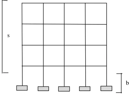
Fig. 1 Structure nodes groupings
In this system of equations, displacement components to which the known support movement belongs can be found in vector xb, while vector xs contains displacements of model nodes to be computed from the support movement. Correspondingly we have partitioned mass matrix M and stiffness matrix K of the structure too. In vector q
( )
tb , there are reaction forces in
direction of the known support vibration. In vector q
( )
tb , there are reaction forces in direction of the known support
vibration.
s
b
M
ss Msb x &&x ts
( )
+ KssK
sb x x ts
( )
= 0M
bs Mbb &&xb
( )
t Kbs Kbb xb( )
t qb( )
tAfter partitioning, the original matrix differential equation can be written in two equations:
( )
( )
( )
( )
M x t M x t K x t K x t
ss s&& + sb b&& + ss s + sb b =0, (2)
( )
( )
( )
( )
( )
M x t M x t K x t K x t q t
bs s&& + bb b&& + bs s + bb b = b . (3)
From the equation
( )
( )
( )
( )
( )
M x t K x t M x t K x t q t
ss s&& + ss s = − sb b&& − sb b = s (4)
that can be written on the basis of Eq. (2), displacements of the structural nodes can be computed, then, vector q
( )
tb of
reaction forces can de defined from Eq.(3).
Displacements of structural nodes originating from support motion can be computed as sum of both effects even if displacements of the individual support points are not identical. A part of the displacement vector -xsst
( )
t - belonging to a given time is the quasi-static displacement computed from support motion values of the given time that can be computed with the assumption that no forces act in the structure nodes, correspondingly, there are no forces of inertia either. The other component of the vector -xsdyn( )
t - is the dynamic displacement of the bar loaded by forces of inertia caused by support motion, i.e.:( )
( )
( )
x ts =xsst t + xsdyn t . (5)
In quasi-static tests, no mass forces are contained in Eq. (2), and for vector xsst
( )
t , from equation( )
( )
K x t K x t
ss s st
sb b
+ =0 (6) the relationship
( )
( )
xsst t K K x t
ss sb b
= − −1 (7)
will be obtained. Then, vector x ts
( )
has the form:( )
( )
( )
x t I K K x t
x t
s
ss sb s dyn
b
= −
−1 . (8)
Substituting this relationship in Eq. (2) and assuming that the mass matrix is a diagonal matrix, for computing xsdyn
( )
t we get the matrix differential equation( )
( )
( )
M x t K x t M K K x t
ss s dyn
ss s dyn
ss ss sb b
&& + = −1 && . (9)
We can see that right-hand side of the system of equations can be generated now in complicated way as computations require matrix K
ss
−1.
DYNAMIC INTERACTION OF STRUCTURES AND SOIL PART
The structure consisting of units with varying damping factor can be theoretically examined applying complex stiffness. Stiffness matrix of a given unit applying complex stiffness is as follows:
(
)
~
K i K
e= +1 γe e, (10)
while complex stiffness matrix can be written in the form
K~= +K iK
i. (11)
Hear if
ϑ
is the logarithmic decrement of vibration structure, thenγ ϑ
π
= . (12) Now, we have to solve the differential equation
( )
( ) ( )
M x t~&& +K x t~~ =q t . (13)
Displacement vector x t
( )
of the dynamic problem will be the real part of vector ~x t( )
.The solution of soil-structure-interaction problem we can calculate in frequency domain. In the earthquake computation model demonstrated by Idriss[1], initial data are displacement unknowns of structure-soil interface points and internal forces resulting in the points even in the no-building case. Equilibrium equation written with complex stiffnesses is in the case of harmonic excitation of given frequency ω:
The complex dynamic stiffness matrix of structure is:
~
K= −K ω2M +i Kγ . (15)
~
x
s is the displacement vector of structural nodes and ~xb is the displacement vector of interface nodes in the finite element model. The soil region is represented by frequency-dependent impedance matrix X~, ~xb* and ~qb *
are the free-field displacements and forces along the interfaces transformed in frequency domain. Impedance matrix X~ can be generated as inverse of complex flexibility matrix and this allows as shown by Wolf [2] also consideration of the radiation damping occurring during wave propagation in the model.
MODAL DECOMPOSITION WITH SPLITTING UP THE DISPLACEMENT VECTOR
For decrease the computing time we can reduce the size of the matrices in the matrix differential equation using the modal decomposition method. On the basis of numerical experiments the necessary number of the eigenvectors is smaller if we break the total displacement amplitudes of the structure into xsst quasi-static displacements introduced by the base response and
xsdyn dynamic displacements of the structural nodes. K~
ss
~ K
sb
x ~ xs
= 0
K~
bs
~ ~ K
X
bb
+
~ xb
~ ~ ~ X x
q
b *
b *
+
This method was used in [3] by Schütz and Wang. Let xsdyn be real part of the complex vector ~xsdyn. Now we write vector ~
xsdyn as combination of real eigenvectors in form of
~ ~
xsdyn =V z. (16) Then, using relationship from Eq. (8):
Introducing notation
P= K− K
ss sb
1 , (18)
after substitution of Eq. (17) into the dynamic equations (14) and multiplying the equations by transported coefficient matrix of Eq. (17) we can get the dynamic equations in form:
After multiplying and using notation
C~=VTK~ −V K P~
sb T
ss . (20)
We can write the dynamic equations (19) in form two matrix differential equation. They are seen in the (21).
~~ ~~ ,
~ ~ ( ~ ~ ~ ~ ~
)~ ~ .
Dz Cx
C z P K P K P P K K X x f + b
T T
ss bs
T
sb bb b b
=
+ − − + + =
0
(21)
Expressing vector ~z from the first equation
~ ~ ~~
z = −D−1C xb. (22) ~
xs =
V −K− K ss sb
1
x ~z
~
xb 0 I ~xb
(17)
T
ss
V K V~ − +
V K P V K T ss T sb ~ ~ x ~ z = 0 − +
P K V
K V T ss bs ~ ~ ~ ~ ~ ~ ~ K X
P K P
P K K P
bb T ss T sb bs + + − − ~
xb ~
f
b
Substituting it into the second equation
(A~− B~−B~T−C D~T~− C~+K~ + X x~) ~ = ~f
bb b b
1
. (23) Here
~ ~
A= PTK P
ss ,
~ ~
B=K P
bs . (24)
Matrix P= K− K
ss sb
1 has matrix K ss
1
− . In large systems it is very difficult to calculate the inverse of the large matrix. But, we can calculate the matrix P in the following equation:
K P K
ss = sb, (25)
and we do not have to calculate the inverse matrix.
In that practical case, when the mass matrix is diagonal matrix and the damping characteristic of the structure is same for all part of structure, the calculating procedure become simpler. In this case the
K~ ( i )K M
ss= +1 ss − s
2
γ ω , (26)
~
( )
K i K M
bb= +1 bb− b
2
γ ω , (27)
K~ ( i )K
sb = +1 γ sb. (28)
Using these matrices:
~
( )
A=P +i K − M P
T
sb s ,
1 γ ω2 (29)
~
( )
B = +1 iγ K P
bs , (30)
and computing the C~ matrix:
~
( ) ( )
C==V +i K − +i K + M P V M P
==
T
sb sb s
T s
1 γ 1 γ ω2 ω2 . (31)
The complex C~ matrix become real matrix. Using this algorithm the computer time can be reduced and we get a good chance to solve the soil-structure interaction problem in the case of large systems. During the calculation it is very important to compute the eigenvectors in the necessary number. In the next we will give some numerical experiments for the necessary number of eigenvectors and we can read more about that in [4].
NUMERICAL EXPERIMENTS
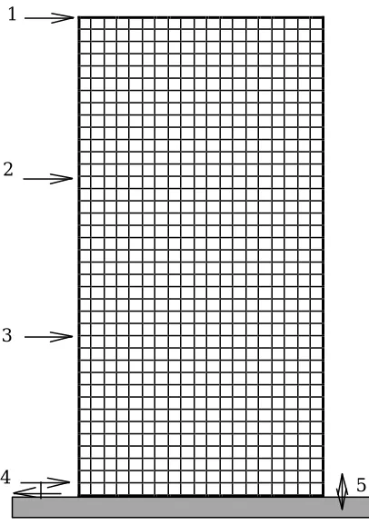
In the case of very flexible structure shown in Fig. 11, the number of degree of freedom was 2400. We calculated the transfer functions of the absolute displacement for horizontal direction of points 1, 2, 3, 4 and the relative displacements to orthogonal to axis and to direct of axis of column at a soil node.
Figures 3.-5. demonstrate the transfer functions for horizontal displacements of structural points 1. and the relative displacements to orthogonal to axis and in direction to axis of the column. Tables 1.-3. show the convergence of maximal values of transfer functions at different values of frequency.
Fig. 2 Model for numerical experiments
0 2 4 6 8 10 12 14 16
ω
x/x0
0 40
Fig. 3 Transfer function of horizontal displacement at 1. point
Table. 1. Maximal values of transfer function of horizontal displacement at 1. point.
ω Direct Number of eigenvectors
[rad/s] solution 1 3 5 10 20 50 100
5,09 13,39 13,39 13,39 13,39 13,39 13,39 13,39 13,39
16,18 4,74 0,52 4,73 4,74 4,74 4,74 4,74 4,74
27,27 2,45 0,41 2,49 2,45 2,45 2,45 2,45 2,45
38,30 1,52 0,34 0,27 1,50 1,52 1,52 1,52 1,52
3 2
5 4
-3 -2,5-2 -1,5-1 -0,50 0,51 1,52 2,53
ω
0
40 (uj-ui)*0.0001
Fig. 4 Transfer function relative displacement orthogonal for axis of the column
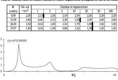
Table 2. Maximal values of transfer function of relative displacement orthogonal for axis of the column
ω Dir. sol. Number of eigenvectors
[rad/s] *10-5 1 3 5 10 20 50 100
4,90 2,20 2,13 2,18 2,19 2,19 2,20 2,20 2,20
15,58 2,40 -0,40 2,13 2,26 2,35 2,39 2,40 2,40
26,30 1,92 -0,14 1,00 1,53 1,79 1,89 1,92 1,92
37,07 1,45 0,16 -1,58 0,69 1,22 1,39 1,45 1,45
0 1 2 3 4 5
ω
(vj-vi)*0,000001
0 40
Fig. 5. Transfer function relative displacement to direction of axis of the column
Table. 3. Maximal values of transfer function of relative displacement to direction of axis of the column
ω Dir. sol. Number of eigenvectors
[rad/s] *10-7 1 3 5 10 20 50 100
5,09 4,28 4,27 4,27 4,27 4,27 4,27 4,28 4,28
15,96 1,44 0,46 1,39 1,40 1,40 1,41 1,43 1,43
28,02 0,63 0,24 0,49 0,53 0,55 0,60 0,62 0,62
In the Table 4. we can see the ratio of computer time in case of different number of eigenvectors (t) to computer time of direct solution (T). Computing time in case of modal decomposition about 10% of the computing time using direct solution.
Table. 4. Ratios of computer times of modal decomposition and direct solution
Number of eigenvectors t/T
5 0,05
10 0,05
20 0,07
50 0,12
100 0,32
CONCLUSION
The solution of soil-structure-interaction problem we can calculate in frequency domain. In the basic equations the structure with internal damping has a complex dynamic stiffness matrix and the soil region is represented by frequency dependent complex impedance matrix.
Calculating the modal amplitudes of the structure fixed at its base we can calculate the displacement vector of interface nodes and using this vector we will get the displacement vector of structural nodes too. This method is very comfortable, but we have to calculate the eigenvectors of a large system. In case of large systems, it is not possible to calculate all the eigenvectors but for a solution of an accuracy required for practical application, it is not necessary either to have all the components.
From the basis of numerical experiments the necessary number of the eigenvectors will be less if we break the total displacement amplitudes of the structure into quasi-static displacements introduced by the base response and dynamic displacements of the structural nodes. In the practical cases if the internal damping is proportional the calculation of the matrices will be simpler. Using this algorithm the computer time can be reduced and we get a good possibility to solve the soil-structure-interaction problem in case of large system.
ACKNOWLEDGEMENT
The author thanks for supporting the research by the Hungarian Scientific Research Fund (OTKA No. T 029635) REFERENCES
1. Idriss, I. M. (chairman), "Analysis for soil-structure interaction effect for nuclear power plants", ASCE, New York, 1979. 2. Wolf, J. .P., "Dynamic Soil-Structures Interaction", Prentice-Hall, Inc., Englewood Cliffs, New Jersey, 1985.
3. Schütz, W., Wang, S., "Soil-Structures-Interaction Analysis in Frequency Domain Using Fixed Base Eigenvalues", Proc. of the 13th International Conference on Structural Mechanics in Reactor Technology (SMiRT-12/K), pp. 139-144, 1993.