ABSTRACT
LINCOLN, KELSEY JEAN. Potential Mechanisms Underlying a Perceived White Bass Morone chrysops Decline in a Southeastern Reservoir. (Under the direction of Dr. D. Derek Aday and Dr. James A. Rice).
Little is known about fundamental aspects of the life history, ecology, and population dynamics of White Bass, Morone chrysops, a popular sport fish in southern reservoirs. In addition, concern regarding possible declining White Bass populations in some North Carolina reservoirs has made the management of this species difficult as the mechanisms associated with these perceived declines are not well understood. Our study aimed to address these knowledge gaps through quantification of two potential mechanisms: Mortality (both fishing, F, and natural, M) and potential interactions with invasive White Perch Morone americana. This study also aimed to increase the general knowledge base on reservoir White
Potential Mechanisms Underlying a Perceived White Bass Morone chrysops Decline in a Southeastern Reservoir
by Kelsey Lincoln
A thesis submitted to the Graduate Faculty of North Carolina State University
in partial fulfillment of the requirements for the degree of
Master of Science
Fisheries, Wildlife and Conservation Biology
Raleigh, North Carolina 2014
APPROVED BY:
_______________________________ ______________________________
Dr. D. Derek Aday Dr. James A. Rice
BIOGRAPHY
I was born in Ann Arbor MI and grew up Canton MI, a once-small town filled with farm land and forests. It was in Canton where I spent many hours exploring the woods and ponds in our backyard. Summers spent camping on the Little Muskegon River in Michigan and growing up in a state with a lake culture are what sparked my interest in aquatic
ecosystems.
I graduated from Salem High School in 2006 and moved on to Michigan State
University to pursue a B.S. in Fisheries and Wildlife. Choosing a degree was easy for me, as I was blessed with a childhood filled with great outdoor experiences. I wanted a career where I could work toward keeping the beautiful lakes and their intricate ecosystems intact for future generations to experience. After graduation in 2010, I worked at the USGS Great Lakes Science Center as a student contractor on a river restoration project aimed to rebuild spawning populations of Lake Sturgeon and Lake Whitefish in the Detroit River. It was during my time at the Great Lake Science Center that I gained the confidence and experience needed to pursue a master's degree.
ACKNOWLEDGMENTS
I would like to first thank the people who supported and helped me through this project at North Carolina State University, especially my advisors Drs. D. Derek Aday and James A. Rice, first, for giving me this opportunity and then for coaching me through it, always providing enough advice to allow me to grow as an individual and a scientist. I could not have accomplished certain aspects of this project without the help I received from Dr. Joseph Hightower. I owe a lot of the initial support and help in designing and preparing for this project to Daniel Brown. A special thanks to graduate students Dr. Marybeth Brey, Dr. Lindsay Campbell, Zachary Feiner, Bethany Galster, Adriane Gill, Augustin Engman, Michael Cove, Michael Fisk, Caitlin Bradley, Mary Henson, Xavier Jamie, and Henry Flowers who graciously volunteered their time and knowledge to help me. Finally, I would like to thank Dylan Owensby for being my patient technician and for putting up with me in countless hours of help in the field and in the lab.
I would also like to thank Brian McRae, Kevin Dockendorf, Corey Oakley, Christian Waters, and Jessica Baumann from the North Carolina Wildlife Resources for their role in creating this project and the knowledge and advice they contributed in planning this project. Jessica Baumann and Corey Oakley were also a great help with field work in the spring. I would also like to thank the North Carolina Wildlife Resources Commission for funding this research through Federal Aid in Sport Fish Restoration grant F-101.
TABLE OF CONTENTS
LIST OF TABLES ... v
LIST OF FIGURES ... vi
POTENTIAL MECHANISMS UNDERLYING A PERCEIVED WHITE BASS MORONE CHRYSOPS DECLINE IN A SOUTHEASTERN RESERVOIR ... 1
INTRODUCTION ... 1
METHODS ... 5
Study Site ... 5
Telemetry... 6
Mortality ... 7
White Bass Interactions with White Perch ... 9
Movement and Habitat ... 12
RESULTS ... 12
Telemetry... 13
Mortality ... 13
White Bass Interactions with White Perch ... 14
Movement and Habitat Use ... 15
DISCUSSION ... 16
REFERENCES ... 23
TABLES ... 27
FIGURES ... 32
ESTIMATION OF WHITE BASS POPULATION PARAMETERS AND POTENTIAL HABITAT OVERLAP WITH WHITE PERCH IN JORDAN LAKE, NC ... 38
INTRODUCTION ... 38
METHODS ... 40
Study Site ... 41
Population Parameters ... 41
Distribution and Habitat ... 42
RESULTS ... 44
Population Parameters ... 44
Distribution and Habitat ... 45
DISCUSSION ... 46
REFERENCES ... 50
TABLES ... 52
FIGURES ... 54
LIST OF TABLES
Table 1.1 Mean length (SD) and weight (SD) of fish implanted with acoustic V9-2L transmitters in 2012 and 2013...27 Table 1.2 Annual and monthly fishing (F), natural (M), and total (Z) instantaneous
mortality rates, total mortality (A), survival (S), exploitation rate (u) and natural mortality (v) for White Bass in Jordan Lake in 2012 and
2013...28 Table 1.3 Schoener’s Index values of diet overlap between all sizes of White Bass
combined (Total White Bass) and all sizes of White Perch combined (Total White Perch) in January and April 2013 as well as between small, medium, and large size classes of both species. A sample size too small for analysis is indicated by *; significant overlap indicated in bold...30 Table 1.4 Results from 2013 stable isotope analysis by species and size class, including
sample size (N), the Bayesian standard ellipse (SEAb)(lower, upper quartile), mean δ13C (SE), δ13C range (CR), mean δ15N (SE), and the δ15
N range
(NR)...31 Table 2.1 Transmitter schedules for White Bass tagged in March 2012 and April 2013
(V9-2L) and for White Perch tagged in October 2012 (V7-4L). The duration of each time step is given in days. The random delay time interval, when a transmitter emits a signal, is shown by number of seconds in parentheses for each step...52 Table 2.2 Number of fish PIT tagged and number of additional fish scanned for tags in
years 2011-2013, mean length (SD), and mean weight (SD) of White Bass sampled for the mark-recapture study in the mouth of the Haw River during the spring spawning run in April 2011, and March and April 2012. Note fish tagged with acoustic tags in 2013 were also implanted with PIT
LIST OF FIGURES
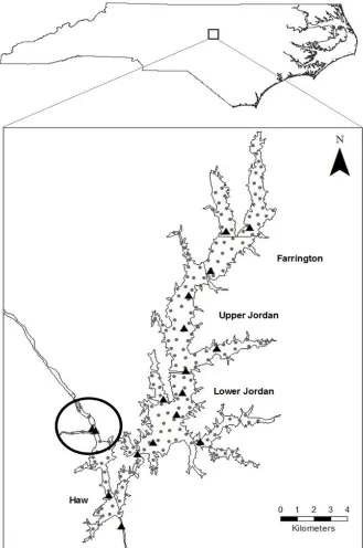
Figure 1.1 Map of Jordan Lake showing its location in central North Carolina, the tagging site in the mouth of the Haw River (black circle), sub-basins of the reservoir (labeled and delineated by gray lines), and locations of VR2W receivers (black triangles) and listening points (gray dots) used for passive and active tracking...32
Figure 1.2 Instantaneous monthly fishing (F, upper panel) and natural (M, lower panel) mortality rates (solid lines) of White Bass in Jordan Lake from April 2012-August 2013. Dashed lines indicate 0.975th and 0.025th credible
intervals...33 Figure 1.3 Diet compositions of White Bass and White Perch collected in January 2013
and April 2013 for (a) all sizes combined, (b) small, medium, and large fish of both species in January 2013, and (c) small, medium, and large fish of both species in April 2013. Size groups with sample sizes too small for analysis were excluded...34 Figure 1.4 Bayesian standard ellipse area (SEAb) for small (thinnest gray ellipse),
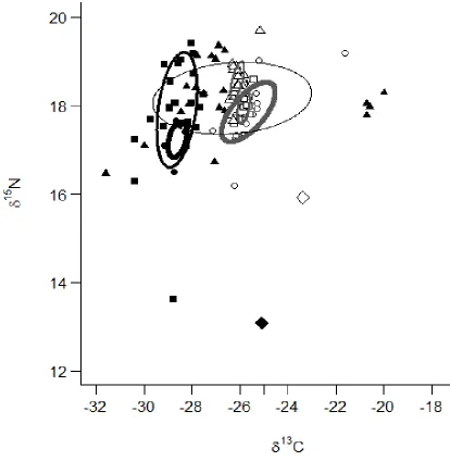
medium (medium thickness gray ellipse), and large (thickest gray ellipse) White Bass and small (thickest black ellipse), medium (medium thickness black ellipse), and large (thinnest black ellipse) White Perch. Isotopic values for individual fish for small (white circles), medium (white squares) and large (white triangles) White Bass as well as small (black circles), medium (black squares) and large (black triangles) White Perch, the pelagic baseline (large white diamond) and the benthic baseline (large black triangle) are
shown...35 Figure 1.5 Seasonal variation, from spring 2012 through summer 2013, in (a) distance to
shore and (b) depth where fish were relocated; heavy lines indicate medians, boxes indicate upper and lower quartiles, bars indicate maximum and
minimum values, and circles indicate outliers; n is the number of
observations...36 Figure 1.6 White Bass distributions during (a) the whole study, (b) spring 2012, (c)
Figure 2.1 White Perch tagging sites in October 2012 (black circles) and combined White Bass tagging site in March 2012 and April 2013 and White Perch tagging site in October 2012 (dashed black circle). Receiver locations (black triangles) and White Bass listening points (solid gray circles) are also
included...54 Figure 2.2 The von Bertalanffy Growth curve for White Bass collected via gillnet
sampling throughout Lower Jordan and the Haw River arm in January 2013 and via electrofishing in mouth of the Haw River in April 2013...55 Figure 2.3 Age distribution of White Bass collected via gillnet sampling throughout
Lower Jordan and the Haw River arm in January 2013 and electrofishing in the mouth of the Haw River in April 2013. Sample sizes are indicated above each bar...56 Figure 2.4 Length frequencies of White Bass collected by electrofishing in the mouth of
the Haw River in April 2011, March and April 2012, and April 2013, and by gillnetting throughout Lower Jordan and the Haw River arm in January
2013...57 Figure 2.5 The distributions of (a) White Bass and (b) White Perch from October
2012-May 2013. Density of fish (fish ), estimated from active tracking data is shown as the background gray scale. Black squares indicate passive receivers; size of the symbol increases with the number of unique fish detected per receiver...58 Figure 2.6 Comparisons of (a) distance to shore and (b) depth of relocated White Bass
and White Perch from October 2012-May 2013; heavy lines indicate medians, boxes indicate upper and lower quartiles, bars indicate maximum and
minimum values, and circles indicate outliers; n is the number of
POTENTIAL MECHANISMS UNDERLYING A PERCEIVED WHITE BASS MORONE CHRYSOPS DECLINE IN A SOUTHEASTERN RESERVOIR
INTRODUCTION
The White Bass Morone chrysops, native to the Mississippi River basin, is a popular sport fish in Midwestern and southern reservoirs. Reports indicate that White Bass are among the most commonly harvested species in Nebraska (Bauer 2002), Texas (Betsill and Pitman 2002), and South Dakota (Willis et al. 2002). White Bass exhibit high growth rates and are highly fecund, contributing to their success as a sport fish (Lee et al. 1980). Despite, or perhaps because of, their popularity, concern regarding declining White Bass populations began in the Great Lakes (Madenjian et al. 2000) when the abundance of age-0 White Bass sharply declined in the 1980s. Similar concerns expressed for some reservoir populations initiated an American Fisheries Society symposium (Guy et al. 2002a, and associated papers) that focused on White Bass ecology and management, and aimed to improve understanding and management of the species. Despite these efforts many reservoir populations may be declining and we still have a limited understanding of the underlying mechanisms. This project aimed to address some of the mechanisms that may be affecting White Bass populations.
quantify monthly fishing and natural mortality when dealing with potentially declining populations.
between White Perch and, in particular, juvenile White Bass (Feiner et al. 2013a). Thus, although stomach content and stable isotope analyses indicate that competitive interactions may exist, questions still remain about the importance of these interactions and their potential to affect White Bass populations.
In addition to the uncertainty over competitive interactions and mortality rates, fishery biologists and managers currently lack a clear understanding of White Bass life history related to important parameters such as seasonal habitat use and distribution patterns. For example, while it is known that reservoir White Bass make a spring migration (Muoneke 1994; Willis et al. 2002; Betsill and Pittman 2002), little is known about their habitat use and distribution throughout the lacustrine portion of the system during non-spawning periods. Use of telemetry to follow seasonal distribution patterns would yield information about how White Bass use lake systems after spawning, and would allow us to contextualize intra-annual variation in mortality rates and identify where potential competitive interactions are occurring. Further, White Bass have often proven to be difficult to sample year round
(Colvin 2002b). Identifying key habitats or distribution patterns throughout the year may aid in more effective sampling apart from the spawning run. We are aware of only one telemetry study that provides information on reservoir distribution throughout the year (Willis et al. 2002).
estimate instantaneous monthly and annual fishing and natural mortality of White Bass, (2) compare diet and niche overlap between White Bass and White Perch through stomach content and stable isotope analysis, and (3) use telemetry to examine habitat use and movement patterns of reservoir White Bass throughout the year in Jordan Lake, a large, eutrophic southeastern reservoir.
METHODS Study Site
B. Everett Jordan Reservoir (Jordan Lake) is a relatively shallow impoundment (mean depth of 5 m; Wong et al. 1999) located in the Piedmont region of North Carolina originally created for flood control (Figure 1.1). Jordan Lake is comprised of four main sub-basins that were assigned names for the purposes of this study; Farrington, Upper Jordan, Lower Jordan, and Haw, the latter including the Haw River arm of the reservoir and the mouth of the river itself (Figure 1.1). Jordan Lake is located near two densely populated cities, Durham and Raleigh, NC, and is a popular lake for recreational activities including sport fishing.
Wildlife Resources Commission (NCWRC) has documented declines in catch rates of White Crappie Pomoxis annularis, Bluegill Lepomis macrochirus, and Flat Bullheads Ameiurus platycephalus, and expressed concerns about potentially declining White Bass (Wong et al.
1999). Telemetry
We used telemetry to estimate mortality and address the spatial components of this study, movement and habitat use. White Bass were collected using boat electrofishing in spring 2012 and 2013 in the Haw River during the spawning run (Figure 1.1). Sampling was conducted by NCWRC and North Carolina State University personnel. We surgically implanted VEMCO (VEMCO, Ltd., Nova Scotia, Canada) V9-2L (29 x 7 mm; 4.7 g) acoustic coded transmitters into 50 White Bass weighing more than 235 g, generally greater than 270 mm, in March 2012 and 25 White Bass in April 2013. Transmitters were pre-programmed to include a passive and an active tracking period over a 30 day cycle; during the active tracking period transmitters emitted a signal every 15-45 s and for the remaining days the transmitters emitted a signal at a slower rate (110-390 s) or were off (Table 2.1). Following Murray (2002), fish were placed in a 64-L induction tank containing 100 mg/L Tricaine methanesulfonate (MS-222). Anesthetized fish were transferred to a surgery table and water containing a maintenance dose of 50 mg/L MS-222 was continuously pumped over the gills. Using a sterile scalpel an incision was made just below the pelvic fins and a
Cornelia, GA). After surgery, fish recovered in a 64-L holding tank before being released. A 30 day pilot study found 100% tag retention in similarly-sized hybrid White Bass X Striped Bass Morone saxatilis, so we assumed zero tag loss in released White Bass.
We used a combination of passive and active approaches to relocate fish. From March 2012-October 2013 we relied on an array of continuously operating VEMCO VR2W
receivers placed strategically throughout the lake to detect large scale movement of tagged fish (Figure 1.1). In the Haw River arm of the reservoir, about 1,500 m below the mouth, we set a gate consisting of two receivers placed approximately 500 m apart to detect upstream and downstream movement during the spawning run. To detect potential escapement from the reservoir, a receiver was placed 400 m downstream of the B. Everett Jordan Dam.
We conducted 19 monthly active tracking efforts from April 2012-October 2013. To ensure full coverage of the study system we established a series of listening points
approximately 700 m apart throughout the lake (Figure 1.1). We listened for 90 s at each listening point, first with a VEMCO VR165 omnidirectional hydrophone and, when a fish was detected, a VR110 directional hydrophone to determine specific location. This approach provided a radius around each listening point of about 350 m (less than the detection range of our tags) and some degree of overlap in coverage (Figure 1.1). Using known locations of test tags placed in the water we determined our location accuracy to be within 2 m.
Mortality
was created in OpenBUGS v. 3.2.2 (© Free Software Foundation, Inc. 2007) using the capture history as the input. This model also built upon other previous models that used telemetry to estimate mortality (Hightower et al. 2001) and was created in conjunction with an additional telemetry mortality model that is under development (J. Hightower,
unpublished data). This model consisted of a state process, including the true state of the fish in time t given the fish's state in time t-1, and an observational process, which was the
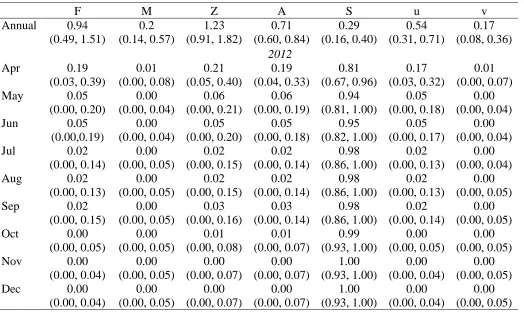
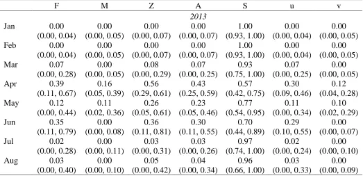
probability of observing each fish's capture history in time t given the fish's state in time t. The observation matrix consisted of three probabilities in which a fish was either detected alive, detected and determined to have died from a natural mortality, or not detected. In the state matrix individual fish were determined to be alive, dead due to a natural mortality, or harvested. Monthly F and M were used to calculate monthly and annual total mortality (A), survival (S), exploitation (u), and natural mortality (v). Annual estimates were obtained by first averaging the monthly instantaneous rates for F, M, and Z estimated over 17 months, then scaling that average to a 12 month period.
Although we could not directly observe fish, any fish relocated in the same spot for three consecutive months was categorized as a natural mortality (Bendock and
Alexandersdottr 1993). A fish no longer located in the system was assumed to have been harvested. Additional model assumptions were: (1) transmitter loss or failure was negligible, (2) there was no catch-and-release mortality, (3) undetected emigration did not occur, (4) no tagged fish were removed from the system via predation, (5) every fish had an equal
other. To ensure that mortalities were not due to surgery we omitted any passive relocation data less than two weeks after tagging.
White Bass Interactions with White Perch
To assess potential competition for resources, White Perch and White Bass were collected for stomach content and stable isotope analysis. Diet overlap was compared in January and April 2013. For the winter stomach content analysis, White Bass were collected in January 2013 by using overnight offshore gillnets set by the NCWRC throughout Lower Jordan and Haw (Figure 1.1). Two types of gill nets were used: the first was an experimental gill net that consisted of seven individual panels of 38-, 44-, 51-, 57-, 64-, 70-, 76-mm bar mesh sizes randomly distributed in 8.7 m sections across a single gill net. The other type was a single mesh gill net that consisted of uniform 38-, 51-, or 64-mm bar mesh size across each individual net. White Bass were sorted into small, medium, and large size bins (≤240 mm, 241-300 mm, and >300 mm) and placed on ice until our goal of 15 fish in each size category was met (our goal was not always met; Chapter 1 Results). White Perch used for stomach content analysis in January 2013 were collected by setting two 2 m x 38 m nearshore experimental mesh gillnets, consisting of five 7.6 m panels of 12.7, 19.1, 25.4, 38.1, and 50.8-mm bar mesh sizes and three 2 x 50 m nearshore gillnets consisting of 25.4-mm bar mesh in the lower basin of the lake, Lower Jordan. Nets soaked for 4-6 hours during the day. White Perch were also sorted into small, medium, and large size classes (≤120 mm, 121-160 mm, >160 mm) and collected until our goal of at least 15 fish in each size class was obtained. White Bass and White Perch were also collected for diet analysis in April 2013, via
collected. The first 15 White Bass collected from each size class during spring electrofishing were used for SIA in addition to diet analysis. To collect White Perch for SIA in April 2013 we followed the same sampling procedure as in January 2013. We aimed to collect White Perch from the lake to use for SIA because stable isotopes provide a temporally integrated measure of food consumption, and we assumed White Bass remained in the lake a majority of the year. Pelagic and littoral baseline samples for SIA were also collected in spring 2013. For the pelagic baseline, we collected zooplankton from several pelagic sites throughout Lower Jordan. Phytoplankton and predatory zooplankton were removed in the laboratory. We used a Ponar grab to take benthic samples near shore, typically in 0.5-1.0 m of water, to collect Chironomidae larvae for the benthic baseline.
In the laboratory, stomachs for stomach content analyses were removed and contents were emptied into vials containing 70% ethanol. Contents of White Perch and White Bass stomachs were sorted into individual categories of prey, including fish, Chironomids, other benthic invertebrates, zooplankton, various eggs, and other (which included detritus, rocks, and mussels). For each stomach individuals in each prey category were counted and weighed in aggregate to the nearest 0.01 g. Categories weighing less than 0.01 g were assigned a weight of 0.005 g.
To quantify diet overlap we first calculated percent frequency of occurrence (% FO), one of the more robust diet measurements relative to percent weight, percent volume, and percent number (Baker et al. 2014). We used Schoener's Index to calculate diet overlap as follows:
where Cxy is the Schoener's Index between species or size class x and species or size class y, Pxi is the % FO of diet item i for species or size class x, and Pyi is the % FO of diet item i for
species or size class y (Schoener 1970). Schoener's Index ranges from 0 (no overlap) to 1 (absolute overlap) and a value of 0.6 or higher was used as a threshold to indicate significant
diet overlap (Wallace 1981).
Stable isotope analysis was done by removing a 12 x 12 mm cube of muscle tissue below the dorsal fin of each fish and sending it to the Cornell University Stable Isotope Lab, where ratios of heavy to light nitrogen isotopes (δ15N) and carbon isotopes (δ13
C) were measured using a Finnigan MAT Delta Plus isotope ratio mass spectrometer (IRMS). Because nitrogen isotopes are typically assumed to have an enrichment factor of 3.4‰ with each increase of trophic level, δ15
N is often used to determine trophic level (Owens 1987). It was our intention to calculate trophic level following the equations developed in Post et al. (2002), however we were unable to do so due to inadequate baseline values that would have resulted in potentially inaccurate trophic level calculations. We ultimately used ANOVA in program R v 2.15.1 to test for differences in mean δ15N and mean δ13
C among the size classes of White Bass and White Perch.
To compare isotopic niche overlap between White Bass and White Perch in all size classes we used Stable Isotope Bayesian Ellipses in R, or SIBER, a Bayesian model developed by Jackson et al. (2011) to calculate and plot the Bayesian standard ellipse area (SEAb), or the isotopic niche area of each species and size class. This model used δ13
or pelagic resources (Post 2002) and δ15
N of individual fish to calculate the SEAb, or isotopic niche area, for each size class for each species. Trophic niche overlap and the general trophic position of each size class for both species could then be compared by plotting the SEAb (δ13C as the x-axis and δ15
N as the y-axis). Movement and Habitat
Each time a fish was located during active tracking we recorded water depth, distance to shore, substrate type (predominately sand, silt, or gravel), and Global Positioning System (GPS) coordinates of the location. For the purposes of analysis monthly habitat and
distribution data were aggregated by spring (April-June), summer (July-September), fall (October-December), and winter (January-March). We used Kolmogorov-Smirnov tests conducted in R to determine whether lake depth or distance to shore varied seasonally. Substrate was homogeneous across fish locations so no statistical analyses were conducted.
To characterize seasonal distributions of tagged White Bass we analyzed relocation data from passive and active tracking in Microsoft Excel 2007 (Microsoft® 2007) and ArcGIS Desktop 10 (© Copyright 2013 Esri). To do this, two separate files were created for every season. The first file converted individual fish locations from active tracking to a density parameter (fish per km2) using the point density tool in ArcGIS 10. The second used the number of unique fish detected on each passive receiver per season, and scaled the size of the symbol representing each receiver relative to the number of fish detected. We then combined these two files to create seasonal maps depicting seasonal distribution and high use areas.
Telemetry
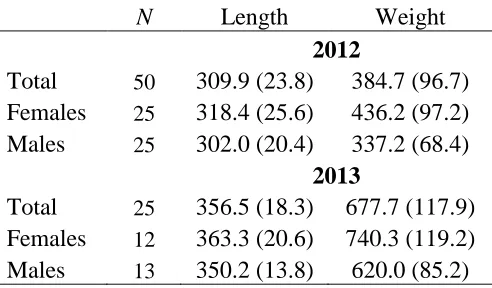
Tagged fish measured 309.9±23.8 mm (mean±SD) in 2012 and 356.5±18.3 mm in 2013 (Table 1.1). An equal number of males and females were tagged each spring (Table 1.1). There were no suspected surgery related deaths in 2012 and three surgery related deaths in 2013, which were censored from analysis. Receivers, continuously monitoring from March 2012-October 2013, recorded a combined total of 480,511 detections for 72 unique fish. Only one emigrating fish was detected on the receiver below the dam, and was subsequently censored from analysis. Monthly tracking efforts from April 2012-October 2013 resulted in a total of 371 fish relocations. By the end of the study (October 2013) only five fish remained with active tags in the system. Transmitters from 2012 were expected to expire late August 2013 and thus our mortality estimate only extended to August 2013. Mortality
White Bass Interactions with White Perch
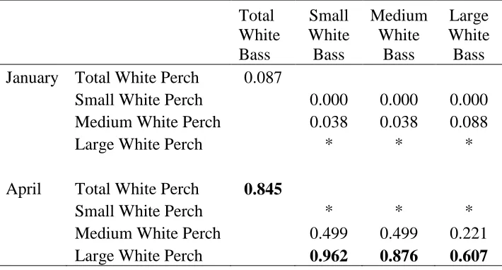
For diet analysis, we collected 74 White Bass in January 2013, 65 (12 small, 14 medium, 39 large) with stomach contents and 45 White Perch, 35 (16 small, 15 medium, 4 large) with stomach contents. Of 48 White Bass collected in April 2013, 31 (8 small, 7 medium, 16 large) had food in their stomachs, and 30 (1 small, 15 medium, 14 large) of 49 White Perch contained stomach contents. Different patterns in diet composition among size classes occurred in January and April. In January 2013, minute diet overlap occurred
between all size classes of White Bass and White Perch (Schoener's Index: 0.087; Table 1.3), as White Bass fed almost exclusively on fish and White Perch consumed mostly
zooplankton, Chironomids and other benthic invertebrates (Figure 1.3a). More specifically, no significant overlap was found among size classes of White Bass and White Perch in January 2013 (Figure 1.3b; Table 1.3). However, in April 2013, White Bass increased their consumption of Chironomids and other benthic invertebrates and decreased fish consumption resulting in a greater and significant overlap with White Perch (Schoener's Index: 0.845), which mostly consumed Chironomids and benthic invertebrates (Figure 1.3a; Table 1.3). In particular, significant overlap occurred between large White Perch and all sizes of White Bass; however, because White Bass became more piscivorous with increasing size, the greatest overlap occurred between large White Perch and small White Bass (Schoener's Index: 0.96; Figure 1.3c; Table 1.3).
Our stable isotope analysis revealed minor differences in δ13
C and δ15N between White Bass and White Perch. White Bass had significantly higher δ15
Bass had greater δ15N values than small White Perch (Tukey’s HSD: df=99; P=0.001; Table 1.4). The isotopic values for the pelagic (15.9, -23.4; δ15
N, δ13C) and benthic (13.28, -25.0) baselines did not appear to be typical baseline values for the species we used or the system (Feiner et al. 2013a) and thus trophic level was not calculated. Mean δ13
C values varied significantly (ANOVA: F=11.55; df=99; P<0.001) between White Bass and White Perch, and particularly between small and medium White Perch and large White Bass (Tukey’s HSD: P≤0.01; Table 1.4); no significant difference (Tukey’s HSD: P≥0.76) was found
between large White Perch and small, medium and large White Bass.
The Bayesian standard ellipse areas (SEAb) for each size class of both species revealed variation in trophic niches as size increased for both species. White Perch ellipse size increased directly with fish size; small to medium White Perch increased their δ15
N range (NR) and medium to large White Perch increased their δ13
C range (CR; Figure 1.4; Table 1.4). Conversely, White Bass ellipse area decreased with increasing fish size and all size classes remained similar in δ13C and δ15N ranges (Figure 1.4; Table 1.4). This resulted in a great deal of niche overlap between large White Perch and all size classes of White Bass. Due to small White bass having the largest SEAb of the White Bass size classes, the greatest overlap appeared to occur between large White Perch and small White Bass. There was no observable niche overlap between the small and medium White Perch and all size classes of White Bass (Figure 1.4).
Movement and Habitat Use
mostly pelagic throughout the year as 83% of fish relocations were at 50-300 m from shore. Distance to shore and depth at location were not correlated (r= 0.0039). Fish were located farther from shore in the winter (148±35 m; mean±SE) compared to spring 2012 (60±31 m) and spring 2013 (63±14 m; Kolmogorov–Smirnov test: D≥0.365; P ≤0.07; Figure 1.5a). Fish
were also located in deeper water in the winter than all other seasons (Kolmogorov–Smirnov test: D≥0.35; P<0.01; Figure 1.5b). White Bass concentrated in several large areas of the
lake and their movement between these high-use areas as well as between sub-basins of the lake varied seasonally and annually (Figure 1.6). High-use areas were mostly located
throughout the deepest sub-basins, the Haw River arm and Lower Jordan (Figure 1.6). While fish tended to move between sub-basins from one high use area to another, generally using the lower, deeper basins the most (Figure 1.6a), some variation in lake use occurred between years and cohorts of tagged fish. For example, in 2012, 30% of tagged fish immediately dispersed to Upper Jordan and Farrington within two weeks and 60% were detected using these uppermost basins throughout the remainder of spring 2012 (April-June). In contrast, in spring 2013 both newly tagged White Bass and surviving fish tagged in 2012 did not disperse as quickly or as much as newly tagged fish in 2012. Only 12% of fish tagged in 2012 used the uppermost basins during April-June 2013. None of the fish tagged in 2013 moved into the uppermost basins within two weeks after tagging and only 16% of them were detected in the upper basins throughout spring 2013.
DISCUSSION
fishing mortality (54%) was greater than all previous estimates we are aware of, which range from 15-35% in Missouri reservoirs (Colvin 2002a) and 11-40% in Kansas reservoirs (Shultz and Robinson 2002). Conversely, the annual natural mortality was lower (17%) in our study than in Kansas reservoirs (56%; Shultz and Robinson 2002). The general lack of published natural mortality estimates precludes making broader comparisons; however, our results indicate that fishing mortality may be affecting White Bass populations more than natural mortality. Heavy exploitation has been shown to lead to increased fluctuations in abundance (Anderson et al. 2008). Heavily truncated age distributions, such as the distribution we observed in Jordan Lake where no fish older than age 4 were found, are often a result of high exploitation rates. This appears to be a common occurrence in reservoir White Bass
populations, especially in southern systems (Colvin 2002; Lovell and Maceina 2002; Chapter 2). White bass recruitment often is highly erratic (Colvin 2002a; Ahrens et al. 2010) and can vary with factors such as prey base (Shultz et al. 2002) and reservoir inflow (DiCenzo and Duval 2002; Shultz et al. 2002), resulting in variable year-class strength. High mortality due to fishing pressure over successive years combined with highly variable recruitment could, therefore, be affecting the abundance of White Bass in Jordan Lake and other reservoir populations.
populations that also experience low natural mortality, such as the population in Jordan Lake (Guy et al. 2002b; Lovell and Maceina 2002). Given the significant fishing mortality
estimated in this study, reducing the bag limit (currently 25 fish a day in North Carolina) may also be an effective option. This might cause an in increase in catch-and release mortality (indistinguishable from natural mortality in our model), however, there may still be an overall increase in the number of mature individuals remaining in the system, especially during the spawning run when fishing mortality peaks. Before adjusting harvest restrictions, creel surveys to quantify metrics such as the catch-and-release rate, the number of White Bass kept each fishing period, the timing of peak fishing pressure during the spawning run, overall fishing pressure, size of harvested fish, and the types of bait used may be useful to determine how effective additional restrictions will be.
While our model shows clear seasonal patterns in fishing and natural mortality, it also has several limitations. First, our assumption of no catch-and-release mortality may have been violated. Anecdotal observations indicated that some anglers did release White Bass, so catch-and-release mortality could potentially be contributing to the high natural mortality rates we estimated during the spring when fishing pressure increases. Currently there are no estimates, to our knowledge, of catch-and-release mortality for reservoir White Bass
populations. Combining telemetry tags with tag return data from traditional tags has been used to estimate catch-and-release mortality and may be a useful adaptation to our model (Bacheler et al. 2009). Our model also could not distinguish between predation (e.g.,
models applied to aquatic acoustic telemetry models. One remedy could be to use radio telemetry tags, which have a better terrestrial range, to determine bird or mammal predation and compare estimates to our results. Ultimately, failure to separate bird and mammal predation from harvest would result in an inflated F whereas failure to separate indirect fishing mortality, due to catch and release, from natural mortality would result in a deflated F. It seems unlikely in our study that removal of tagged fish via predation would have been
common enough to inflate our estimates of F given the large size of tagged fish and their tendency to remain offshore and in deep water. Catch-and-release mortality during the spring spawning run could have resulted in the underestimation of F; given that our estimate is already relatively high, however, that possibility would not change the interpretation of our data. .
costly period when fish may be experiencing higher than normal rates of natural mortality (Guy et al. 2002b). Although some apparent natural mortality may actually be due to catch-and-release mortality, a spike in natural mortality after spawning may be expected due to the associated energetic costs. Finally, as diet overlap with White Perch increased substantially during the spring, potential competition may be adding stress during this time if resources are limited. Restrictive harvest limits and additional enforcement might be options to mitigate the increased mortality experienced by White Bass during their spawning run.
throughout the lake and the river. Evidence from this study and previous studies (Kuklinski 2007; Feiner et al. 2013a) is consistent and suggests that overlap between adult White Perch and juvenile White Bass poses the greatest potential for competition (other than possible overlap during earlier life history stages that hasn't been evaluated). Given limited resources, that could be a contributing factor in declining White Bass populations in reservoirs where White Perch are established (Feiner et al. 2013a).
Stable isotope analysis can be powerful tool for fishery scientists to better understand trophic interactions and intricate food webs in aquatic ecosystems, however, quality baseline samples are necessary to obtain reliable trophic level estimates. This proved difficult in our study as our baseline samples did not appear to accurately represent their assumed baseline trophic position. In particular, the isotopic values for the benthic baseline (Chironomids), assumed to be δ13
C enriched from consuming plant material and algae in the littoral zone (Peterson and Fry 1987), were actually more δ13
C depleted than the pelagic baseline. Chironomids have been shown to exhibit high intraspecific variability among individuals from the same lake depending on life stage and where samples were collected (Grey et al. 2004). It is possible the individuals we collected were more δ13
C depleted than other individuals and were thus not representative of the true baseline. In addition, both the benthic and pelagic baselines were δ15N enriched, and only slightly below the δ15
N values of our fish. Finally, the δ15
N values for White Bass (17.9, 18.6; min, max) and White Perch (17.2, 18.2) from our system appeared to be greater than the δ15
N of White Bass (12.5, 14.9) and White Perch (10.8, 11.9) in Lake James, another North Carolina reservoir, but similar to the δ15
2013b), suggesting that Jordan Lake may be more nitrogen enriched than other systems. Even though we could not estimate trophic levels in this study, the relative comparison of δ15N and δ13
C values among species and size groups is valid, which allowed us to confidently interpret the pattern of niche overlap between large White Perch and all size classes of White Bass.
The movement and distribution patterns we observed for White Bass did not suggest any localized habitats, such as sandy coves or areas with woody debris, where competitive interactions with White Perch might be significant, but it did provide insight as to how White Bass use reservoirs outside of their predictable spawning run. Difficulty in locating White Bass for efficient sampling outside the spawning season is a common problem in managing White Bass populations (Colvin 2002b). Our study provided evidence of predictable
patterns, similar to those found by Willis et al. (2002), showing that White Bass concentrated relatively far offshore and in deep waters during the winter. These patterns, in addition to the high-use areas we identified, may aid in increasing the efficiency and effectiveness of
REFERENCES
Anderson, C.K., C. Hsieh, S.A. Sandin, R. Hewitts, A. Hollowed, J. Beddington, R.M. Mays, and G. Sugihara. 2008. Why fishing magnifies fluctuations in fish abundance. Nature 452:835-839.
Ahrens, A.E., T.W. Shaeffer, M..R. Wuellner, and D.W. Willis. 2010. Population and diet assessment of White Bass in Lake Sharpe South Dakota. The Prairie Naturalist 42:130-137.
Bacheler, N.M., J.A. Buckel, J.E. Hightower, L.M. Paramore, and K.H. Pollock. 2009. A combined telemetry – tag return approach to estimate fishing and natural mortality rates of an estuarine fish. Canadian Journal of Aquatic Sciences 66: 1230-1244.
Baker, R., A. Buckland, and M. Sheaves. 2014. Fish gut content analysis: robust measures of diet composition. Fish and Fisheries 15:170-177.
Bauer, D. 2002. White Bass population differences in Nebraska reservoirs with Gizzard Shad or Alewife prey bases. North American Journal of Fisheries Management 22:665-670. Bendock, T. and M. Alexandersdottr. 1993. Hooking mortality of Chinook Salmon released
in the Kenai River, Alaska. North American Journal of Fisheries Management 13:540-549.
Boileau, M.G. 1985. The expansion of White Perch, Morone americana, in the Lower Great Lakes. Fisheries Vol 10:1.
Betsill, R. and V. Pitman. 2002. Comparison of creel statistics for river and reservoir components of a Texas White Bass fishery. North American Journal of Fisheries Management 22:659-664.
Busch, W.N., D.H. Davies, and S.J. Nepszy. 1977. Establishment of White Perch, Morone americana, in Lake Erie. Journal of the Fisheries Research Board of Canada 34:1039-1041.
Colvin, M. 2002a. Population and fishery characteristics of White Bass in four large Missouri reservoirs. North American Journal of Fisheries Management 22:677-689.
DiCenzo, V. and M. Duval. 2002. Importance of reservoir inflow in determining White Bass year-class strength in three Virginia reservoirs. North American Journal of Fisheries Management 22:620-626.
Feiner, Z.S., J. A. Rice, A.J. Bunch, and D.D. Aday. 2013a. Trophic niche and diet overlap between invasive White Perch and resident White Bass in a southeastern reservoir. Transactions of the American Fisheries Society 142:912-919.
Feiner, Z.S., J.A. Rice, and D.D. Aday. 2013b. Trophic niche of invasive white perch and potential interactions with representative reservoir species. Transactions of the American Fisheries Society 142:628-641.
Grey, J., A. Kelly, S. Ward, N. Sommerwerk, and R. Jones. 2004. Seasonal changes in the stable isotope values of lake dwelling Chironomid larvae in relation to feeding and life cycle variability. Freshwater Biology 49:681-689.
Guy, C., R. Schultz, and M. Colvin. 2002a. Ecology and management of White Bass. North American Journal of Fisheries Management 22:606-608.
Guy, C, R.D. Schultz and C.A. Cox. 2002b. Variation in gonad development, growth, and condition of White Bass in Fall River Reservoir, Kansas. North American Journal of Fisheries Management 22:643-651.
Hsieh, C., A. Yamauchi, T. Nakazawa, W. Wang. 2010. Fishing effects on age and spatial structures undermine population stability of fishes. Aquatic Sciences 72:165–178. Harris, J.L. 2006. Impacts of the invasive White Perch on the fish assemblage of Kerr
Reservoir Virginia. Master's Thesis. Virginia Polytechnic Institute and State University, Blacksburg, Virginia.
Hightower, J., J. Jackson, and K. Pollock. 2001. Use of telemetry methods to estimate natural and fishing mortality of Striped Bass in Lake Gaston, North Carolina. Transactions of the American Fisheries Society 130:557-567.
Jolly, G.M. 1965. Explicit estimates from capture-recapture data with both death and immigration-Stochastic model. Biometrika 52:225-247.
Kery, M., M. Schaub. 2011. Bayesian Population Analysis using WinBUGS: A hierarchical perspective. Academic Press, Waltham, Massachusetts.
Lee, D. S., C. R. Gilbert, C. H. Hocutt, R. E. Jenkins, D. E. McAllister, and J. R. Stauffer, Jr. 1980. Atlas of North American freshwater fishes. North Carolina State Museum of Natural History, Raleigh, NC.
Lovell, R., and M. Maceina. 2002. Population assessment and minimum length limit evaluations for White Bass in four Alabama reservoirs. North American Journal of Fisheries Management 22:609-619.
Madenjian, C. P., R. L. Knight, M. T. Bur, and J. L. Forney. 2000. Reduction in recruitment of White Bass in Lake Erie after invasion of White Perch. Transactions of the
American Fisheries Society 129:340-1353.
Murray, M.J. 2002. Fish surgery. Seminars in Avian Exotic Pet Medication 11:246–257. Martin, D. R., L.A. Powell, and K.L. Pope. 2009. Spring home ranges of White Bass in
irrigation reservoirs of the Republican River basin, Nebraska. Ecology of Freshwater Fish, 18:514-519.
Muoneke, M.I. 1994. Dynamics of a heavily exploited Texas White Bass population. North American Journal of Fisheries Management 14:415-422.
Owens, N.P. 1987. Natural variations in I5N in the marine environment. Advanced Marine Biology 24:389-451.
Peterson, B.J., B. Fry. 1987. Stable Isotopes in Ecosystem Studies. Annual Review of Ecology and Systematics 18:293-320.
Post, D. M. 2002. Using stable isotopes to estimate trophic position: Models, methods, and assumptions. Ecology 83:703-718.
Pollock, K.H., J. D. Nichols, J. E. Hines, and C. Brownie. 1990. Statistical inference for capture–recapture experiments. Wildlife Monographs 107.
Seber, G.F. 1965. A note on the multiple recapture census. Biometrika 52:249-259.
Schultz, R. and D. Robinson. 2002. Exploitation and mortality rates of White Bass in Kansas reservoirs. North American Journal of Fisheries Management 22:652-658.
Scott, W.B. and W.J. Christie. 1967. The invasion of the lower Great Lakes by White Perch Roccus americanus (Gmelin). Journal of the Fisheries Research Board of Canada 20:1189-1195.
Schoener, T.W. 1970. Non-synchronous spatial overlap of lizards in patchy habitats. Ecology 51:408-418.
Wallace Jr., R.K. 1981. An assessment of diet-overlap indexes. Transactions of the American Fisheries Society 110:72-76.
Willis, D.W., C.P. Paukert, and B.G. Blackwell. 2002. Biology of White Bass in eastern South Dakota Glacial Lakes. North American Journal of Fisheries Management 22:627-636.
Wong, R. K., R. L. Noble, J.R. Jackson, and S.V. Horn, S. V. 1999. White Perch invasion of B. Everett Jordan Reservoir, North Carolina. Proceedings of the Southeastern
TABLES
Table 1.1: Mean length (SD) and weight (SD) of fish implanted with acoustic V9-2L transmitters in 2012 and 2013.
N Length Weight
2012
Total 50 309.9 (23.8) 384.7 (96.7) Females 25 318.4 (25.6) 436.2 (97.2) Males 25 302.0 (20.4) 337.2 (68.4)
2013
Table 1.2: Annual and monthly fishing (F), natural (M), and total (Z) instantaneous mortality rates, total mortality (A), survival (S), exploitation rate (u) and natural mortality (v) for White Bass in Jordan Lake in 2012 and 2013.
F M Z A S u v
Annual 0.94 (0.49, 1.51) 0.2 (0.14, 0.57) 1.23 (0.91, 1.82) 0.71 (0.60, 0.84) 0.29 (0.16, 0.40) 0.54 (0.31, 0.71) 0.17 (0.08, 0.36) 2012
Apr 0.19
(0.03, 0.39) 0.01 (0.00, 0.08) 0.21 (0.05, 0.40) 0.19 (0.04, 0.33) 0.81 (0.67, 0.96) 0.17 (0.03, 0.32) 0.01 (0.00, 0.07)
May 0.05
(0.00, 0.20) 0.00 (0.00, 0.04) 0.06 (0.00, 0.21) 0.06 (0.00, 0.19) 0.94 (0.81, 1.00) 0.05 (0.00, 0.18) 0.00 (0.00, 0.04)
Jun 0.05
(0.00,0.19) 0.00 (0.00, 0.04) 0.05 (0.00, 0.20) 0.05 (0.00, 0.18) 0.95 (0.82, 1.00) 0.05 (0.00, 0.17) 0.00 (0.00, 0.04)
Jul 0.02
(0.00, 0.14) 0.00 (0.00, 0.05) 0.02 (0.00, 0.15) 0.02 (0.00, 0.14) 0.98 (0.86, 1.00) 0.02 (0.00, 0.13) 0.00 (0.00, 0.04)
Aug 0.02
(0.00, 0.13) 0.00 (0.00, 0.05) 0.02 (0.00, 0.15) 0.02 (0.00, 0.14) 0.98 (0.86, 1.00) 0.02 (0.00, 0.13) 0.00 (0.00, 0.05)
Sep 0.02
(0.00, 0.15) 0.00 (0.00, 0.05) 0.03 (0.00, 0.16) 0.03 (0.00, 0.14) 0.98 (0.86, 1.00) 0.02 (0.00, 0.14) 0.00 (0.00, 0.05)
Oct 0.00
(0.00, 0.05) 0.00 (0.00, 0.05) 0.01 (0.00, 0.08) 0.01 (0.00, 0.07) 0.99 (0.93, 1.00) 0.00 (0.00, 0.05) 0.00 (0.00, 0.05)
Nov 0.00
(0.00, 0.04) 0.00 (0.00, 0.05) 0.00 (0.00, 0.07) 0.00 (0.00, 0.07) 1.00 (0.93, 1.00) 0.00 (0.00, 0.04) 0.00 (0.00, 0.05)
Dec 0.00
Table 1.2 Continued
F M Z A S u v
2013
Jan 0.00
(0.00, 0.04) 0.00 (0.00, 0.05) 0.00 (0.00, 0.07) 0.00 (0.00, 0.07) 1.00 (0.93, 1.00) 0.00 (0.00, 0.04) 0.00 (0.00, 0.05)
Feb 0.00
(0.00, 0.04) 0.00 (0.00, 0.05) 0.00 (0.00, 0.07) 0.00 (0.00, 0.07) 1.00 (0.93, 1.00) 0.00 (0.00, 0.04) 0.00 (0.00, 0.05)
Mar 0.07
(0.00, 0.28) 0.00 (0.00, 0.05) 0.08 (0.00, 0.29) 0.07 (0.00, 0.25) 0.93 (0.75, 1.00) 0.07 (0.00, 0.25) 0.00 (0.00, 0.05)
Apr 0.39
(0.11, 0.67) 0.16 (0.05, 0.39) 0.56 (0.29, 0.61) 0.43 (0.25, 0.59) 0.57 (0.42, 0.75) 0.30 (0.09, 0.46) 0.12 (0.04, 0.28)
May 0.12
(0.00, 0.44) 0.11 (0.02, 0.36) 0.26 (0.05, 0.61) 0.23 (0.05, 0.46) 0.77 (0.54, 0.95) 0.11 (0.00, 0.34) 0.10 (0.02, 0.29)
Jun 0.35
(0.11, 0.79) 0.00 (0.00, 0.08) 0.36 (0.11, 0.81) 0.30 (0.11, 0.55) 0.70 (0.44, 0.89) 0.29 (0.10, 0.55) 0.00 (0.00, 0.07)
Jul 0.02
(0.00, 0.28) 0.00 (0.00, 0.11) 0.03 (0.00, 0.31) 0.03 (0.00, 0.26) 0.97 (0.74, 1.00) 0.02 (0.00, 0.24) 0.00 (0.00, 0.10)
Aug 0.03
Table 1.3: Schoener’s Index values of diet overlap between all sizes of White Bass
combined (Total White Bass) and all sizes of White Perch combined (Total White Perch) in January and April 2013 as well as between small, medium, and large size classes of both species. A sample size too small for analysis is indicated by *; significant overlap indicated in bold.
Total White Bass
Small White Bass
Medium White
Bass
Large White Bass January Total White Perch 0.087
Small White Perch 0.000 0.000 0.000
Medium White Perch 0.038 0.038 0.088
Large White Perch * * *
April Total White Perch 0.845
Small White Perch * * *
Medium White Perch 0.499 0.499 0.221
Table 1.4: Results from 2013 stable isotope analysis by species and size class, including sample size (N), the Bayesian standard ellipse (SEAb)(lower, upper quartile), mean δ13
C (SE), δ13C range (CR), mean δ15N (SE), and the δ15
N range (NR).
N SEAb δ13C CR δ15N NR
White Bass Total 52 -25.9 (0.10) 5.5 18.1 (0.08) 6.4
Small 19 2.13 (1.8, 2.5) -25.6 (0.25) 5.5 17.9 (0.15) 3.0 Medium 14 0.80 (0.7, 0.95) -25.8 (0.07) 0.8 18.0 (0.10) 1.3 Large 19 0.75 (0.64, 0.87) -26.1 (0.06) 1.3 18.6 (0.10) 2.0
White Perch Total 48 -27.7 (0.35) 11.6 17.9 (0.15) 5.8
FIGURES
Figure 1.2: Instantaneous monthly fishing (F, upper panel) and natural (M, lower panel) mortality rates (solid lines) of White Bass in Jordan Lake from April 2012-August 2013. Dashed lines indicate 0.975th and 0.025th credible intervals.
0.0 0.1 0.2 0.3 0.4 0.5 0.6 0.7 0.8
Apr May Jun Jul Aug Sep Oct Nov Dec Jan Feb Mar Apr May Jun Jul Aug
0.0 0.1 0.2 0.3 0.4 0.5 0.6 0.7 0.8
Figure 1.5: Seasonal variation, from spring 2012 through summer 2013, in (a) distance to shore and (b) depth where fish were relocated; heavy lines indicate medians, boxes indicate upper and lower quartiles, bars indicate maximum and minimum values, and circles indicate outliers; n is the number of observations.
ESTIMATION OF WHITE BASS POPULATION PARAMETERS AND POTENTIAL HABITAT OVERLAP WITH WHITE PERCH IN JORDAN LAKE, NC
INTRODUCTION
Although the White Bass Morone chrysops is a popular sport fish in many
southeastern and Midwestern reservoirs, relatively little is known about its life history and ecology in lentic systems (Guy et al. 2002a). In addition, there have been concerns that White Bass are declining in some reservoirs, but the mechanisms associated with these declines are not well understood, making management of this species especially difficult. Several mechanisms contributing to population declines have been suggested, including high fishing mortality (Muoneke 1994; Chapter 1) and competitive interactions with invasive White Perch Morone americana (Gopalan et al. 1998; Madenjian 2000; Kuklinski 2007; Feiner 2013a, 2013b; Chapter 1). However, it remains difficult to make management decisions based on these potential mechanisms because our overall understanding of White Bass population dynamics is limited.
Information on population size, growth rates, and age structure can substantially enhance our ability to assess potential declines and associated mechanisms in White Bass populations. An estimate of population size can provide a valuable indication of status as well as provide a baseline from which to monitor fluctuations or trends. However, collecting a representative sample large enough to estimate population size (typically via
spawning adults (Colvin 2002b). Growth rates and age structure of White Bass are also important as both parameters can influence population fluctuations and recruitment. White bass growth rates are known to vary widely among systems (Colvin 2002a), between sexes (Guy et al. 2002b), and by prey base (Bauer 2002). Data on age structure can provide information on the proportion of mature adults in the population and whether or not the population is dominated by strong year-classes. Although White Bass can live up to 14 years (Willis et al. 2002), many reservoir White Bass populations exhibit highly truncated age distributions, with few fish surviving past age 5 (Bauer 2002; Colvin 2002a; Lovell and Maceina 2002; Willis et al. 2002; Chapter 1). Colvin (2002a) found that annual mortality rates increased from 40% to 80% after age 4. Fluctuations in population abundance and truncated size and age distributions have historically been linked to high fishing mortality from over-exploitation (Anderson 2008). Thus, obtaining basic information on White Bass population characteristics is an important first step in understanding population dynamics and possible declines.
none directly evaluate the extent of overlap in habitat use or distribution patterns of these two species in systems where they co-occur. Despite being a common invasive species most movement studies of White Perch occur in their native range (McGrath 2005; Divver 2012). White Bass are typically thought to have large home ranges (Martin et al. 2009), whereas White Perch exhibit relatively small home ranges (McGrath 2005). White Bass are typically thought of as an open water pelagic species, whereas White Perch are a more littoral species using habitats with flat bottoms and sandy or soft substrates (Stanley and Danie 1983). In reservoirs, White Bass exhibit diel movement patterns and spring migrations related to spawning (Willis et al. 2002; Divver 2012). Though White Perch in their native range migrate to spawn in rivers, tributaries, or estuaries, very little is known about the seasonal distribution of White Perch in invaded systems. Thus, understanding whether White Bass and White Perch exhibit similar seasonal distribution patterns or occupy similar habitats may provide additional insight to where and when competitive interactions may be occurring.
The goal of this study was to quantify several key White Bass population parameters while also evaluating habitat and distribution similarities with White Perch in a southeastern reservoir where managers are concerned about a potential White Bass population decline. Our main objectives were to (1) estimate White Bass spawning population size using a mark-recapture approach, (2) determine White Bass growth and age structure, and (3) assess
Study Site
This study used the same study site, B. Everett Jordan Reservoir (Jordan Lake), and study design as a larger ongoing study investigating White Bass spatial distribution and mechanisms that could be causing their decline (Chapter 1). Jordan Lake was impounded in 1981 and White Perch wee first detected in 1988 (Wong et al. 1999). Thus, Jordan Lake is an excellent reservoir for comparing White Perch and White Bass habitat use and distribution patterns in a system as both species are well established.
Population Parameters
To estimate population size, we conducted a mark-recapture study from 2011-2013. Our approach was to use a modified mark-recapture model in which a sub-sample of the population is marked and re-marked over multiple occasions to estimate population size (N), apparent survival (φ), the number of new individuals entering the system (β), and the
We collected White Bass for age analysis during winter gillnetting and spring electrofishing in 2013. White Bass and White Perch that were brought back to the lab for stable isotope analysis and stomach content analysis (Chapter 1) in January 2013 and April 2013 were also used for age analysis. Both winter and spring fish samples were kept on ice and brought back to the laboratory where sagittal otoliths were removed. Otoliths were cleaned with water and soap, embedded in epoxy, sectioned transversely using a Buehler IsoMet® Low Speed Saw, mounted on a slide, and aged using a Nikon SMZ1000
microscope with a polarized lens. Otoliths were aged by two independent readers.
Disagreements between the first two readers (which only happened twice), were resolved by an independent third reader. To estimate growth we fit mean length at age using the von Bertalanffy growth curve in OpenBUGS v. 3.2.2 (© Free Software Foundation, Inc. 2007) with the following equation:
where lt is the estimated length at age t, L∞ is the asymptotic length at which growth reaches zero, K is the estimated growth rate, and to is the estimated age at which lt equals zero (Ricker 1975). We also examined the White Bass length frequency distribution by combining the length data from White Bass collected during all sampling efforts in 2011-2013.
Distribution and Habitat
April 2012 (N=50) and March 2013 (N=25) as part of a more extensive study (Chapter 1). Data for White Perch were obtained from 20 fish implanted with VEMCO V7-4L (22.5 x 7 mm; 1.8 g) in October 2012, when White Perch reached a taggable size. White Perch weighing greater than 50 g, typically greater than 160 mm, were collected in the evening using boat electrofishing at three sites (identified as areas where White Bass concentrated during that particular time in our study) throughout Jordan Lake and the Haw River arm (Figure 2.1; Chapter 1). We followed the same surgery protocol and guidelines used for transmitter implantation in White Bass (Chapter 1). Both transmitter types were
programmed to include passive and manual tracking periods when transmitters emitted a signal at slower or faster rates for intervals during a 30 day cycle (Table 2.1).
coinciding active tracking periods for both species, when transmitters emitted a signal every 15-45 s. The White Perch transmitters were designed to extend battery life and due to a smaller battery had a shorter tracking period (3 days) than the transmitters used in White Bass (5-12 days). To ensure the entire lake was searched, we created a series of listening points placed approximately 600-700 m apart for White Bass and 400-500 m apart for White Perch. At each point, we listened using a VEMCO VH165 omnidirectional hydrophone; if a fish was detected we then used a VEMCO VH110 directional hydrophone to locate the fish. At each fish location, we recorded the depth of the water column (m), distance to shore (m), substrate type (predominately sand, silt, or gravel), and the exact location using a Global Positioning System (GPS). To analyze the distribution data we combined active and passive tracking data of White Bass and White Perch from October 2012-May 2013. Using the program ArcGIS Desktop 10 (© Copyright 2013 ESRI), we created a series of files using the same protocol as in Chapter 1 to map their seasonal distribution. We tested for differences in the distributions of distance to shore and depth at location between species using a
Kolmogorov-Smirnov test in R v 2.15.1 (© Free Software Foundation, Inc. 2007). RESULTS
Population Parameters
consulting in 2013 revealed that a reliable population estimate was not feasible based on our collections to date, thus, no additional fish were PIT tagged in 2013 (apart from fish
implanted with acoustic transmitters that also received PIT tags). Our low recapture rate (<1.0%) indicated that a much higher number of tagged fish would have been needed to obtain the precision required for an accurate estimate.
We aged 125 White Bass collected in 2013. Of these, 74 fish were obtained during January gillnetting and 51 were obtained from April electrofishing. In both cases fish from all size classes were collected. White Bass exhibited rapid growth (K=0.67±0.13;
median±SD), reaching approximately 290 mm TL by age 2 with an asymptotic length of nearly 400 mm (L∞= 396.6±19.7 mm; to =-0.31±0.19; Figure 2.2). The White Bass population in Jordan Lake was dominated by young fish (≤age 2) and exhibited a heavily truncated age distribution with ages ranging from 1-4 (Figure 2.3). In 2011 there appeared to be one year class dominating the size distribution consisting of fish ranging in size from 220-280 mm (likely age 1). This year class also dominated the size distribution in 2012 at age 2, ranging from 280-340 mm, and again at age 3 ranging from 340-380 mm in 2013 (Figure 2.4). In 2012 and 2013, the age-1 year class was not as pronounced as the 2011 age-1 year class. No young of the year White Bass were collected.
Distribution and Habitat
release, two White Perch were never detected and six were suspected mortalities by November. Thus, only White Perch that survived and were detected past November were used in our analysis (N=12). Distribution patterns between the two species during this time period varied slightly (Figure 2.5), however, due to the low number of White Perch
relocations and because our comparisons for White Perch are based on 12 individuals, these results are inconclusive. Mainly, White Perch remained in the same sub-basin they were tagged in and did not move between sub-basins, whereas White Bass tended to move between sub-basins and exhibited seasonal movement patterns (Chapter 1). For example, 79% of White Perch were detected using only one sub-basin, whereas only 21% of White Bass were detected using one sub-basin October 2012-May 2013. Neither species appeared to concentrate in any particular habitat, but White Bass were located slightly closer to shore than White Perch (Kolmogorov–Smirnov test: D=0.392; P=0.028; Figure 2.6a). As an example, 87% of White Perch relocations were at 50-300 m from shore, whereas only 54% of White Bass relocations were at 50-300 m from shore. In addition, White Perch were never located less than 50 m from shore. White Bass and White Perch were located at similar lake depths of around 5 m (Figure 2.6b).
DISCUSSION
Our results revealed a White Bass population with a heavily truncated age
less than age 4 and rarely found fish greater than age 7. Similarly, Lovell and Maceina (2002) found 98% of fish sampled in four Alabama reservoirs were younger than age 5. This truncated age distribution may be indicative of over exploitation. High fishing mortality due to over exploitation may be causing an increase in population abundance fluctuations
(Anderson 2008). Frequent fluctuations in abundance, especially after consecutive years of low abundance, may lead managers to believe populations are declining. Truncated age distributions and population fluctuations may be sustainable, but are heavily reliant on the production of strong year-classes every 3-4 years (Lovell and Maceina 2002). While we observed one strong year class throughout this study, White Bass experience highly erratic recruitment (Shultz et al. 2002; Ahrens et al. 2010) resulting in erratic year-class strength (DiCenzo and Duval 2002). Failure to produce a strong year class every 3-4 years could potentially devastate a White Bass population.
The fast growth rate of White Bass found in this study was consistent with other studies. White Bass growth in Jordan Lake (K=0.67) appeared to fall within the growth rate range (K=0.50-0.89) found in four large Missouri reservoirs (Colvin 2002a). The asymptotic length found in this study (L∞= 396.6 mm) also appeared to fall within a normal range found in other reservoirs. For example, Colvin (2002) found that White Bass asymptotic length varied from 396-449 mm. High growth rates allow many White Bass populations to reach their asymptotic length by age 3-4 (Lovell and Maceina 2002). However, according to our results, White Bass in Jordan Lake may not reach their asymptotic length until after age 4.
assess whether a minimum length limit is a successful management strategy for White Bass, as few states have enforced this practice (Muoneke 1994). Muoneke et al. (1994) found moderate benefits after instating minimum length limits in a previously unregulated Texas reservoir; generally speaking, the average fish size increased and more anglers practiced catch-and-release. Simulations of White Bass population dynamics in four Alabama
reservoirs suggested that populations experiencing fast growth and high fishing mortality as well as a natural mortality rate of less than 30% may benefit from enforcing minimum length limits (Lovell and Maceina 2002). White Bass in Jordan Lake exhibited a relatively high growth rate, an especially high fishing mortality rate and a low natural mortality rate (Chapter 1), suggesting that minimum length limits could be useful in reducing impacts of fishing on this White Bass population.
Sampling White Bass remains difficult and, although White Bass are relatively abundant and accessible during their spring spawning run, it was not feasible, despite
caught, so had we been able to make an estimate it would have only applied to age-1 and older fish. As White Bass are difficult to sample year-round, obtaining accurate population estimates for the species has become a common problem (Colvin 2002b). A more feasible option for managers may be to focus on relative population abundance through other
sampling methods such as fall gillnetting, suggested by Colvin (2002b) to be the least sex- or age-biased method to use.
REFERENCES
Anderson, C.K., C. Hsieh, S.A. Sandin, R. Hewitts, A. Hollowed, J. Beddington, R.M. Mays, and G. Sugihara. 2008. Why fishing magnifies fluctuations in fish abundance. Nature 452:835-839.
Bauer, D. 2002. White Bass population differences in Nebraska reservoirs with Gizzard Shad or Alewife prey bases. North American Journal of Fisheries Management 22:665-670. Colvin, M. 2002a. Population and fishery characteristics of White Bass in four large Missouri
reservoirs. North American Journal of Fisheries Management 22:677-689.
Colvin, M. 2002b. A comparison of gill netting and electrofishing as sampling techniques for White Bass in Missouri's large reservoirs. North American Journal of Fisheries Management 22:690-702.
Divver, M.M., 2012. Examining the ecological role of White Perch (Morone americana) using acoustic telemetry in the Great South Bay estuary, New York. Master's thesis. Stony Brook University, Stony Brook, New York.
Feiner, Z.S., J. A. Rice, A.J. Bunch, and D.D. Aday. 2013a. Trophic niche and diet overlap between invasive White Perch and resident White Bass in a southeastern reservoir. Transactions of the American Fisheries Society 142:912-919.
Feiner, Z.S., J.A. Rice, and D.D. Aday. 2013b. Trophic niche of invasive white perch and potential interactions with representative reservoir species. Transactions of the American Fisheries Society 142:628-641.
Gopalan, G., D.A. Culver, L. Wu, and B. K. Trauben. 1998. Effects of recent ecosystem changes on the recruitment of young-of-the-year fish in western Lake Erie. Canadian Journal of Fisheries and Aquatic Sciences 55:2572-2579.
Guy, C., R. Schultz, and M. Colvin. 2002a. Ecology and management of White Bass. North American Journal of Fisheries Management 22:606-608.
Guy, C., R.D. Schultz, and C.A. Cox. 2002b. Variation in gonad development, growth and condition of White Bass in Fall River Reservoir, Kansas. North American Journal of Fisheries Management 22:643-651.