Stochastic Search Variable Selection for Identifying
Multiple Quantitative Trait Loci
Nengjun Yi,*
,†,1Varghese George*
,†and David B. Allison*
,†,‡*Department of Biostatistics,†Section on Statistical Genetics,‡Clinical Nutrition Research Center, University of Alabama, Birmingham, Alabama 35294-0022
Manuscript received December 5, 2002 Accepted for publication March 13, 2003
ABSTRACT
In this article, we utilize stochastic search variable selection methodology to develop a Bayesian method for identifying multiple quantitative trait loci (QTL) for complex traits in experimental designs. The proposed procedure entails embedding multiple regression in a hierarchical normal mixture model, where latent indicators for all markers are used to identify the multiple markers. The markers with significant effects can be identified as those with higher posterior probability included in the model. A simple and easy-to-use Gibbs sampler is employed to generate samples from the joint posterior distribution of all unknowns including the latent indicators, genetic effects for all markers, and other model parameters. The proposed method was evaluated using simulated data and illustrated using a real data set. The results demonstrate that the proposed method works well under typical situations of most QTL studies in terms of number of markers and marker density.
M
OST complex traits important to evolution, animal the test on other selected markers to absorb effects of and plant breeding, and medical genetics are in- other QTL. In the last decades, several statistical methods fluenced by the segregation of multiple genes [quantita- have been developed to detect multiple QTL and esti-tive trait loci (QTL)] and environmental factors. There mate their locations and effects simultaneously, includ-is strong interest in inferring the number, genomic loca- ing the multiple-interval mapping approach (Kaoet al. tions, and genetic effects of QTL. Recently, the most 1999; Zeng et al. 2000), variable selection methods widely used methods are interval mapping (Landerand (Ball 2001; Piepho and Gauch 2001; Broman and Botstein1989;HaleyandKnott1992). These meth- Speed2002), and Bayesian methodology with the revers-ods are developed on the basis of a single-QTL model ible-jump Markov chain Monte Carlo algorithm ( Sata-and detect QTL effects at different genomic locations gopan and Yandell 1996; Satagopan et al. 1996; separately. Although these methods have been success- Heath1997;Sillanpa¨a¨andArjas1998;Stephensand fully applied to detect QTL for a number of traits in a Fisch 1998; Xu and Yi 2000; Yi and Xu 2000, 2001; number of organisms, they may result in biased esti- Hoeschele2001). These methods treat mapping multi-mates for QTL locations and effects when the traits are ple QTL as a problem of model determination and actually controlled by multiple, especially linked, QTL variable selection (Sillanpa¨a¨andCorander2002).(e.g.,HaleyandKnott1992). In this study, we propose an alternative Bayesian method
For complex traits governed by multiple QTL, it is neces- for identifying multiple quantitative trait loci in experi-sary to take the whole genome into account for estimating mental designs. Our method is based on a variable selec-the number, locations, and genetic effects of QTL. It has tion method, called stochastic search variable selection been recently shown both theoretically and empirically (SSVS), developed byGeorgeandMcCulloch(1993). that multiple-QTL methods can improve power in de- SSVS was originally introduced for linear regression tecting QTL and eliminate biases in estimates of QTL
models and has been adopted for more complex models locations and genetic effects that can be introduced by
such as generalized linear models (Georgeand McCul-using a single-QTL model (e.g., Haley and Knott
loch1997), log-linear models (Ntzoufraset al.1997), 1992). Composite interval mapping creates a relatively
and multivariate regression models (Brownet al.1998). simple and systematic procedure to map multiple QTL
The difference between SSVS and other variable selec-(JansenandStam1994;Zeng1994). This method
de-tion approaches is that the dimensionality is kept con-tects and estimates each individual QTL by conditioning
stant across all possible models by limiting the posterior distribution of nonsignificant terms in a small neighbor-hood of zero instead of removing them from the model 1Corresponding author: Department of Biostatistics, Ryals Public
as is usually done. Due to this unique property, SSVS is
Health Bldg., 1665 University Blvd., University of Alabama,
Bir-mingham, AL 35294-0022. E-mail: [email protected] able to (1) be easily implemented via the Gibbs sampler,
(2) evaluate each variable effect on the dependent re- and sponse, and (3) provide the posterior probability that
p(xij⫽ ⫺0.5|yi,xi(⫺j),,␣,2e) ⫽1⫺p(xij⫽0.5|yi,xi(⫺j),,␣,2e) , each variable should be included in the model.
(2) In most QTL studies, a large number of markers are
available across the genome, and these markers are usu- where␣ ⫽(␣1, . . . ,␣K),xi(⫺j)⫽(xi1, . . . ,xi(j⫺1),xi(j⫹1), ally closely related. It has been hypothesized that the . . . ,xiK) , the conditional probabilityp(xij⫽ 0.5|xi( j⫺1), genetic variation of most quantitative traits is actually xi(j⫹1)) depends on the recombinant rates between marker controlled by a few loci with large effects and a large j and its flanking markers (j ⫺ 1) and (j ⫹ 1), and number of loci with small effects (e.g., Lynch and p(yi|xi(⫺j),xij⫽0.5,,␣,2
e) is a normal density function
Walsh1998). Therefore, only a small number of mark- with mean ⫹兺K
j⫽1xij␣j and variance 2e. Obviously, ers are expected to have large effects on the trait because the first method ignores the probability distributions of of being linked to large-effect loci, and most of the the missing genotypes and provides approximate esti-markers have nonsignificant effects. Our method con- mates of the missing genotypes. In contrast, the second siders all markers simultaneously and is able to evaluate method can take the probability distributions into ac-not only marker effects of the entire genome, but also count. In this study, we use the second method to de-the posterior probability of each marker having
signifi-scribe our Bayesian approach. cant effects.
Stochastic search marker selection:In variable selection problems, statistical models can be naturally represented by a set of binary indicator variables␥ ⫽ (␥1, . . . ,␥K),
METHODS
where ␥j⫽ 1 or 0 represents the presence or absence
Linear model:We describe the method primarily for of covariatejin the model, respectively. The difference a mapping population with only two segregating geno- between SSVS and other variable selection approaches types, e.g., a backcross, double-haploid lines (DHLs), is that the dimension of parameter space remains un-or recombinant inbred lines (RILs). Assume that we
changed so that the Gibbs sampler can be easily used observe K markers along the genome. Among the K
to explore both the model space and the parameter markers, some may be tightly linked to genes with large
space (GeorgeandMcCulloch1993). effects and therefore have large effects, and others may
The SSVS constructs the prior distribution for (␥, have only weak effects. Our aim here is to identify which
␣) in two stages. The prior distribution of the model markers are tightly linked to genes with large effects
indicator variablesp(␥) is chosen to reflect prior belief and to estimate the magnitude of their effects. For a
in whether particular markers are linked to QTL. A continuously distributed trait, the observed phenotypic
simple choice might have the␥j’s independent, so that value of individuali,yi, can be described by the linear
model,
p(␥)⫽
兿
Kj⫽1
p(␥j). (3)
yi ⫽ ⫹
兺
Kj⫽1
xij␣j⫹ei, (1)
When no information is available, a uniform prior is chosen for each␥j,i.e.,p(␥j ⫽0) ⫽p(␥j⫽ 1)⫽0.5. where is the population mean,xij denotes the
geno-The marker effects␣j(j⫽1, . . . ,K) are given normal type of marker jfor individuali and is defined by 0.5
prior distributions conditional on the corresponding or⫺0.5 for the two genotypes in the mapping
popula-indicators␥j: tion,␣jis the effect size associated with markerj, and
eiis the residual error assumed to followN(0, 2e). ␣
j|␥j ⵑ(1⫺ ␥j)N(0,2j)⫹ ␥jN(0,c2j2j), j⫽1, . . . ,K. (4)
In practice, some marker data may be missing. Two
The prior parameters2
j andc2j are chosen so that2j is methods deal with missing marker data. The first method
“small” andc2
j2j is “large.” Hence, if␥j⫽ 0, the magni-is to replace the mmagni-issing genotype xij by its conditional
tude of the effect␣jis small and then the prior distribu-expectation E(xij|Mi) ⫽ 0.5p(xij ⫽ 0.5|Mi) ⫺ 0.5p(xij ⫽
tion for ␣jforces this parameter to be close to zero. If ⫺0.5|Mi), whereMiis observed marker data for
individ-uali, andp(xij⫽0.5|Mi) andp(xij⫽ ⫺0.5|Mi) are the ␥j⫽1, the magnitude of the effect␣jis large and then conditional probabilities that markerjfor individual i a nonzero estimate of ␣j should be included in the takes the two genotypes, respectively, and can be calcu- model and its posterior distribution will largely be deter-lated using the multipoint method (Jiang and Zeng mined by the data. On the basis of the above prior 1997). The second method is to impute the missing specification, a multivariate normal distribution can be marker genotypes by sampling from the corresponding used as the joint prior distribution for␣conditional on fully conditional probability distribution. Ifxijis missing, ␥, given by
the fully conditional distribution can be derived as
␣|␥ ⵑNK(0,D␥RD␥) , (5)
p(xij⫽0.5|yi,xi(⫺j),,␣,2e)
where R is the prior correlation matrix that is usually assigned to beR⫽IorR⬀(xxT)⫺1, andD
␥⫽ diag[a11,
⫽p(yi|xi(⫺j),xij⫽0.5,,␣,e2)p(xij⫽0.5|xi(j⫺1),xi(j⫹1))
兺
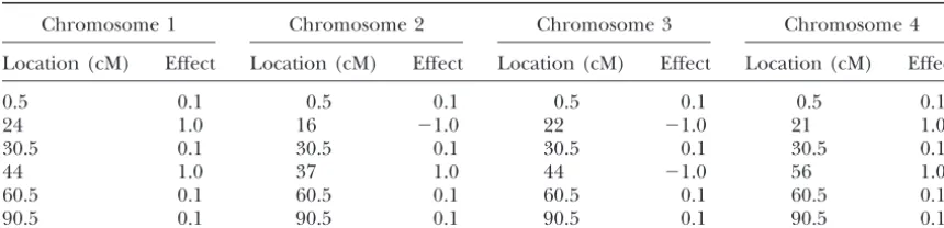
xijp(yi|xi(⫺j),xij,,␣, 2TABLE 1
Locations and effects of simulated QTL
Chromosome 1 Chromosome 2 Chromosome 3 Chromosome 4
Location (cM) Effect Location (cM) Effect Location (cM) Effect Location (cM) Effect
0.5 0.1 0.5 0.1 0.5 0.1 0.5 0.1
24 1.0 16 ⫺1.0 22 ⫺1.0 21 1.0
30.5 0.1 30.5 0.1 30.5 0.1 30.5 0.1
44 1.0 37 1.0 44 ⫺1.0 56 1.0
60.5 0.1 60.5 0.1 60.5 0.1 60.5 0.1
90.5 0.1 90.5 0.1 90.5 0.1 90.5 0.1
prior distribution foris assumed to be NormalN(,2) for convergence is reached. The posterior sample {((t), ␣(t),2
e(t),␥(t)):t⫽ 1, 2, . . . } converges in distribution to with prespecified prior mean and prior variance 2.
The prior for2
eis chosen to be of a scaled inverse⫺2 the joint posterior distribution,p(,␣,2e,␥|y,M). The embedded subsequence {␥(t)
j :t⫽1, 2, . . . } thus con-distribution, Inv⫺ 2(
0,20), with known
hyperparamet-ers0and20. verges top(␥j|y,M),j⫽1, . . . ,K. Generally, the
mark-ers with large effects will appear most frequently and On the basis of the prior specifications described
above, we can use the Gibbs sampler to generate samples quickly, making them easier to identify. Therefore, markers with high posterior probability included in the from the posterior distributionp(,␣,2
e,␥|y,M). Start-ing with an initial value ((0),␣(0),2
e(0),␥(0)), the Gibbs model will most probably be linked to large-effect QTL. sampler proceeds as follows:
1. Sample the missing marker genotypes from the full SIMULATION STUDIES AND REAL DATA ANALYSIS conditional posterior distributions described in
Simulation studies:The applicability of the proposed Equation 2.
method was demonstrated by analyzing simulated data. 2. Samplefrom the full conditional posterior
distribu-The experimental sample was from a backcross and con-tion:
tained 300 segregating individuals. Four chromosomes with length 100 cM each were simulated. Twenty-one
p(|y,x,␣,2 e)⫽N
冢
/2⫹兺n i⫽1(yi⫺兺
K j⫽1xij␣j)/2e
1/2⫹n/2 e
, 1
1/2⫹n/2 e
冣
.
codominant markers were evenly placed on each chro-mosome with marker intervals of 5 cM each. We simu-3. The full conditional posterior distribution of␣is multi- lated 8 large-effect QTL and 16 small-effect QTL
con-variate normal,NK((xxT⫹ 2
e(D␥RD␥)⫺1)⫺1xT(y⫺ ), trolling the expression of a quantitative trait. The 2
e(xxT⫹ 2e(D␥RD␥)⫺1)⫺1). Sampling from this distri- locations of the simulated QTL and their genetic effects bution requires recomputing (xxT⫹ 2
e(D␥RD␥)⫺1)⫺1 are shown in Table 1. The overall mean and the residual on the basis of new values of2
eand␥and thus may be variance were set to be ⫽1 and2e⫽ 1, respectively. costly. To avoid computing (xxT⫹ 2
e(D␥RD␥)⫺1)⫺1, we The genetic variance of QTL j is calculated by vj ⫽ sample ␣j (j ⫽ 1, . . . ,K) from the full conditional a2j/4, where aj is the true genetic effect. Ignoring the posterior distribution p(␣j|y,x,,␣(⫺j), 2e,␥), which covariance due to linkage, the total genetic variances is normal distribution (Wanget al.1994), where␣(⫺j) for the 8 large-effect QTL and 16 small-effect QTL are denotes all terms of␣except␣j. 2 and 0.04, respectively. Therefore, the phenotypic vari-4. Sample2
efrom the full conditional posterior distri- ances explained by each large-effect QTL and each
bution: small-effect QTL are 8 and 0.08%, respectively. We
ran-domly generated missing markers of 10%. The design
p(2
e|y,x,,␣)⫽Inv⫺ 2
冢
0⫹n, 020⫹兺n
i⫽1(yi⫺ ⫺兺 K j⫽1xij␣j)2
0⫹n
冣
. was replicated five times and analyzed using the
pro-posed method. The results averaged over the five repli-cates were reported.
5. Sample␥j fromp(␥j|y,x,␥(⫺j),,␣,2e)⫽p(␥j|␥(⫺j),
For each analysis, the initial values ((0), ␣(0), ,␣,2
e) , which is Bernoulli with probability 2
e(0),␥(0)) were randomly generated from their priors.
p(␥j|␥(⫺j),,␣,2e) We used the uniform distribution as prior for␥as de-scribed earlier. Following the principles developed in
⫽ p(␣|␥(⫺j),␥j⫽1)p(␥j⫽1)
p(␣|␥(⫺j),␥j⫽1)p(␥j⫽1)⫹p(␣|␥(⫺j),␥j⫽0)p(␥j⫽1)
, GeorgeandMcCulloch(1993, 1997) for choosingj
andcj, three different prior variances,i.e., (2j,c2j2j)⫽ (0.001, 10), (0.01, 10), (0.01, 100), were used for the where␥(⫺j)denotes all terms of␥except␥j.
Figure 1.—Simulation study. Posterior probabili-ties of marker indicators (left) and marker effects (right) are plotted against marker locations along the
genome. Red, (2
j,c2j2j)⫽
(0.001, 10); green, (2 j,c2j
2
j)⫽(0.01, 10); blue, (2j, c2
j2j)⫽(0.01, 100).
The prior correlation matrix was assigned to be the samples kept in the post-Bayesian analysis was 10,000 (Gelman et al. 1995). The stored sample was used to identity matrix,i.e.,R⫽I. The prior distribution for
was N(0, 2). The hyperparameter 0 for 2e was set to infer the parameters of interest.
The estimated posterior probabilities for the marker zero, which yields the noninformative prior distribution
p(2
e)⬀ ⫺e2(Gelmanet al. 1995). indicators ␥j (j ⫽ 1, . . . , K) are given in Figure 1
(left). The posterior probabilityp(␥j|y,M) was obtained The Gibbs sampler was run for 50,000 cycles after
discarding the first 2000 cycles for the burn-in period. by counting the number of samples in which the marker indicator␥jis 1, divided by the total of number of sam-It tookⵑ1 hr to generate each sample with a C⫹⫹
pro-gram on a Pentium 4 PC. The chain was thinned (saved ples. As shown in Figure 1, for almost all markers, the posterior probabilities for the first prior setting were one iteration in every 5 cycles) to reduce serial
Figure 2.—Simulation study. Posterior distributions of overall mean and residual variance are shown: (a) overall mean for (2
j, c2
j2j)⫽(0.001, 10); (b) residual
variance for (2
j,c2j2j)⫽(0.001, 10);
(c) overall mean for (2
j, c2j2j) ⫽
(0.01, 10); (d) residual variance for (2
j,c2j2j)⫽(0.01, 10); (e)
over-all mean for (2
j,c2j2j)⫽(0.01, 100);
(f) residual variance for (2 j,c2j2j)⫽
(0.01, 100).
posterior probabilities for the second prior setting were QTL were identified in our analyses. Actually, these QTL had effects close to zero and thus were picked up larger than those for the third. For the three sets of
prior variances, however, the profiles of the posterior only occasionally.
The profiles of marker effects are displayed in Figure 1 probability distributions were similar. These profiles are
very peaked, suggesting that the markers corresponding (right). Although empirical posterior distribution for each marker effect can be depicted, for simplicity we to the peaks have much larger effects than the rest.
From these profiles, we also found that for most situations report only the posterior mean over the samples. The marker effects were estimated to be essentially identical two markers flanking a large-effect QTL have very
differ-ent posterior probabilities, one being large and another for the three sets of prior variances (2
j,c2jj2). Therefore, these prior variances had an ignorable influence on the being close to zero. Therefore, our method may be
powerful in distinguishing closely linked markers. There posterior inference about the marker effects. As in the case of the posterior probability distribution of marker are a total of eight main peaks along the four simulated
chromosomes on the profiles, and two are on one chro- indicators, the profiles of marker effects also have eight obvious peaks, each corresponding to a marker that is mosome. It can be observed that the markers
corre-sponding to the peaks are those that are the closest to the closest to a large-effect QTL. For markers far from the large-effect QTL, their effects were estimated to be the simulated eight large-effect QTL. Therefore, our
Figure 3.—Single-marker regression analysis for chro-mosome 1. (a) Values of
t-test statistic; (b) marker ef-fects.
on the estimated posterior probability of the marker butions of significant markers to be determined by the data.
indicator. When the posterior probability was estimated
to be close to one, the estimate of the marker effect Real data analysis: Data from the North American Barley Genome Mapping Project (Tinkeret al.1996) were was close to the true value. Otherwise, the marker effects
were slightly underestimated. These results are expected analyzed using the proposed Bayesian method. Seven traits were investigated in the project: heading, yield, because the marker effects with the corresponding
indi-cators being zero are forced to be close to zero by the maturity, height, lodging, kernel weight, and test weight. We present only the results of “heading” here. The DH priors. However, we observed that the conditional
esti-mates of marker effects were close to the true value if we (double-haploid) population contained 145 lines (n⫽ 145), each grown in a range of environments. A total used only the posterior samples with the corresponding
indicators equal to one. of 127 mapped markers (K⫽127) covering a 1500-cM
genome along seven linkage groups were used in the The empirical posterior distributions for the overall
mean and the residual variance are depicted in Figure analysis. The average phenotypic values across the envi-ronments were calculated for each line and these aver-2 (a–f). The estimated means for these two parameters
were very close to the simulated values and the standard age values were treated as the original phenotypic values (yi) for the analysis. These phenotypic values were fur-deviations were small, showing that the overall mean
and the residual variance were estimated with precision. ther standardized. The standardized records were used in the analysis.
For comparison, we also performed the single-marker
analyses with the simple regression method for each The prior distributions for (,␣,2
e,␥), the prior variances (2
j,c2j2j), the length of the Gibbs sampler, and marker and the usual multiple regression analysis with
all markers as predictors. For the single-marker analyses, the thinning scheme of the posterior sample were set to be the same as those in the analysis of our simulated the profiles of thet-test statistics and the marker effects
on chromosome 1 are shown in Figure 3. Apparently, data described above. The initial values ((0),␣(0),2 e(0), ␥(0)) were randomly generated from their priors. these two profiles have only one peak covering a wide
range. This shows that the single-marker analyses fail to For the three different prior specifications, the plots of the posterior probabilities of the marker indicators separate the two linked QTL. It is also obvious that the
marker effects were seriously overestimated. Since the are shown in Figure 5, and the marker effects are de-picted in Figure 6. As observed in our simulation studies, marker density is quite high, results of single-marker
analyses should be close to that of the interval mapping. for almost all markers, the posterior probabilities for the first prior setting were larger than those for the other Therefore, the proposed method was shown to be more
powerful than the widely used interval-mapping method two settings, and the posterior probabilities for the sec-ond prior setting were larger than those for the third. for detecting multiple QTL. Figure 4 shows the plot of
the marker effects against the genome location (centi- However, the profiles of the posterior probability distri-butions were proximate. As shown in Figure 6, the marker morgans) of the markers from multiple regression
anal-ysis. Obviously, the effects of most markers far from the effects were estimated to be essentially identical for the three sets of prior variances (2
j,c2jj2). For the first prior large-effect QTL have not shrunk in the usual multiple
regression analysis, indicating that multiple regression setting, it was found that five markers with posterior probabilities from 0.75 to 0.95 and marker effects of failed to detect clear signals of QTL. A common feature
of the proposed Bayesian method and the usual multiple ⵑ ⫾0.4, are located at chromosomes 1, 3, 4, and 6, respectively. We also found five markers on chromo-regression method is that all markers are included in
the model. The clear advantage of the proposed method somes 3, 4, 5, and 6, respectively, with posterior probabil-ities from 0.4 to 0.6. Using the interval mapping of is that it uses two different prior distributions for the
distri-Figure 4.—Marker ef-fects plotted against marker locations along the genome from multiple-marker re-gression analysis.
(1996) declared only three QTL on chromosomes 1, 4, tiple markers. The proposed method was shown to be extremely efficient under typical situations of most QTL and 7, respectively, as significant (data not shown here).
Two markers on chromosome 1 were found to have the studies in terms of the number of markers and the marker density. Compared with the existing Bayesian posterior probability ofⵑ0.76 and the effect ofⵑ⫺0.4.
However,Tinkeret al.(1996) declared only one QTL methods, such as the reversible-jump MCMC, the SSVS approach has advantages on simplicity of computation on chromosome 1 as significant.
For the first prior setting, the posterior means of the and diagnosis of convergence (George and McCul-loch1997). The SSVS procedure can even be imple-overall mean and the residual variance were estimated
to beˆ⫽0.0882 andˆ2
e⫽0.3102, respectively. The pro- mented using the publicly available software BUGS (Congdon2002) and thus can be widely used in QTL portion of phenotypic variance explained by the markers
is calculated ashˆ2⫽(2
y ⫺ ˆ2e)/y2, where2y ⫽1 is the studies.
An essential element of the performance of our Gibbs phenotypic variance for the standardized phenotype.
Thus, the proportion of phenotypic variance explained sampler is its ability to move between two different val-ues of the indicator variable␥j. In the analyses of the by the markers was estimated to be ⵑ69%. From the
estimates of the marker effects ␣ˆj (j ⫽ 1, . . . , K), simulated data and real data, the value of ␥j changed frequently, suggesting that the proposed algorithm we calculated the proportion of phenotypic variance
explained by markerjashˆ2
j ⫽ ␣ˆ2j/4 and found that the mixes well and the chain converges quickly. However, as described inGeorgeandMcCulloch(1993, 1997), proportion of phenotypic variance explained by each
of the five strongest markers wasⵑ4%. convergence can be very slow and thus computational problems can arise whenc2
j is set too large. This setup can lead to very small transition probabilities for␥jto
DISCUSSION
go from 0 to 1 or from 1 to 0. After extensive testing, George andMcCulloch(1997) indicated that these Mapping multiple QTL can be viewed essentially as
problems can be avoided wheneverc2
j ⱕ 10,000. Also, a problem of model selection (e.g.,BromanandSpeed
mixing behavior and convergence of the chain is ex-2002;Sillanpa¨a¨andCorander2002). A variety of
sta-pected to be affected by marker density. In the cases of tistical selection procedures including both
non-Bayes-high-density maps with hundreds of markers, one might ian and Bayesian methods have been developed for
consider a second iteration of SSVS with a reduced conventional statistical models. Some of these
proce-set of markers based on the first run (George and dures have been modified to map multiple QTL. In
McCulloch1993). This two-stage strategy may improve this study, we developed a Markov chain Monte Carlo
accuracy of estimating the marker effects and the poste-(MCMC) algorithm on the basis of the SSVS approach
Figure5.—Posterior prob-abilities of marker indica-tors for heading in barley. Ticks on the horizontal axes represent markers. Red, (2
j, c2
j2j)⫽(0.001, 10); green,
(2
j,c2j2j)⫽(0.01, 10); blue,
(2
j,c2j2j)⫽(0.01, 100).
Recently, Xu (2003) proposed a Bayesian method marker effect, it does not provide a probability state-ment about statistical significance for marker effects. In under the random regression model to simultaneously
estimate genetic effects associated with markers of the our approach, indicator variables are introduced but all effects included in the model have the same prior entire genome in inbred line crosses. In his Bayesian
framework, each genetic effect was assigned a normal variance and all effects excluded from the model have another common prior variance. Therefore, our method prior distribution with mean zero and a unique variance.
The effect-specific prior variance was further assigned not only estimates each marker effect, but also provides the posterior probability that each marker has a signifi-a vsignifi-ague prior so thsignifi-at the vsignifi-arisignifi-ance wsignifi-as estimsignifi-ated from
the data. This approach is analogous to the Bayesian cant effect on the trait. The introduction of indicator variables may allow a large number of markers to be method ofMeuwissenet al.(2001) for BLUP prediction
of gene effects in outbred populations. For a backcross included in the model. It is worth noting that both the random-model approach and our method include all population withKmarkers, Xu’s method needs to
esti-mateKdifferent marker effects␣j(j⫽ 1, . . . ,K) and markers in the analysis and thus may have the ability to control the genetic variances of a large number of small-K different variances 2
j (j⫽1, . . . ,K), where ␣j ⵑ N(0,2
Figure6.—Marker effects plotted against marker loca-tions along the genome for heading in barley. Ticks on the horizontal axes represent
markers. Red, (2
j,c2j2j)⫽
(0.001, 10); green, (2
j, c2j
2
j)⫽ (0.01, 10); blue, (2j,c2j
2
j)⫽(0.01, 100).
in detecting multiple QTL and estimating the genetic puted genotypes are then incorporated into our Bayes-ian procedure. The second approach is to substitute effects deserves further investigation.
We have applied the SSVS approach to identify multi- markers by positions in the marker intervals if we assume that at most one QTL is on any marker interval. This ple QTL by analyzing all markers of the whole genome.
When the markers are densely and regularly spaced, approach requires searching the optimal positions within the marker intervals. The algorithms for updat-the marker analysis would provide reasonable estimates
of marker effects and marker posterior probabilities ing QTL positions have been developed (e.g.,Xu and Yi2000;YiandXu2000, 2001) and can be easily incor-even when QTL are located in the marker intervals. If
the marker density is low and irregularly spaced, how- porated into our procedure.
The SSVS approach has been extended to the multi-ever, the marker analysis will be biased. In these
situa-tions, however, we can extend the proposed method to variate regression model (Brownet al.1998). In QTL-mapping studies, the joint analysis of multiple traits can allow for finer structure mapping by two ways. The first
approach is to use the multiple imputation method to provide formal procedures to test a number of biologi-cally interesting hypotheses concerning the nature of generate the missing genotypes at grids of points
cer-dominant and missing markers in various crosses from two inbred
tain situations, the joint analysis can improve statistical
lines. Genetica101:47–58.
power in detecting QTL and estimating the genetic param- Kao, C. H., Z-B. ZengandR. D. Teasdale, 1999 Multiple interval
mapping for quantitative trait loci. Genetics152:1203–1216.
eters. We can extend the proposed method by applying
Lander, E. S., andD. Botstein, 1989 Mapping Mendelian factors
the SSVS approach to jointly identify QTL for correlated
underlying quantitative traits using RFLP linkage maps. Genetics
multiple traits. In this study, we considered mapping 121:185–199.
Lynch, M., andB. Walsh, 1998 Genetics and Analysis of Quantitative
multiple QTL under the nonepistatic model. A growing
Traits. Sinauer Associates, Sunderland, MA.
number of experiments provide strong evidence of the
Meuwissen, T. H. E., B. J. HayesandM. E. Goddard, 2001
Predic-presence of interactions between genes for many com- tion of total genetic value using genome-wide dense marker maps.
Genetics157:1819–1829.
plex traits. Under the epistatic model, the number of
Ntzoufras, I., J. J. ForsterandP. Dellaportas, 1997 Stochastic
genetic effects increases exponentially as the number
search variable selection for log-linear models. Technical Report.
of markers increases. The multiple-stage SSVS approach Faculty of Mathematics, Southampton University, Southampton,
UK.
can be employed to identify interacting QTL.
Piepho, H.-P., andH. G. Gauch, Jr., 2001 Marker pair selection We are grateful to two anonymous reviewers for their helpful com- for mapping quantitative trait loci. Genetics157:433–444. ments. This work was supported by National Institutes of Health grants Satagopan, J. M., andB. S. Yandell, 1996 Estimating the number R01ES009912, P41RR006009, R01DK054298, and P30DK56336 to D.B.A. of quantitative trait loci via Bayesian model determination. Ab-stracts of the Joint Statistical Meeting, October 1996, Chicago.
Satagopan, J. M., B. S. Yandell, M. A. NewtonandT. C. Osborn, 1996 A Bayesian approach to detect quantitative trait loci using Markov chain Monte Carlo. Genetics144:805–816.
LITERATURE CITED
Sen, S., andG. Churchill, 2001 A statistical framework for
quantita-Ball, R. D., 2001 Bayesian methods for quantitative trait loci map- tive trait mapping. Genetics159:371–387.
ping based on model selection: approximate analysis using the Sillanpa¨a¨, M. J., andE. Arjas, 1998 Bayesian mapping of multiple Bayesian information criterion. Genetics159:1351–1364. quantitative trait loci from incomplete inbred line cross data.
Broman, K. W., andT. P. Speed, 2002 A model selection approach Genetics148:1373–1388.
for the identification of quantitative trait loci in experimental Sillanpa¨a¨, M. J., andJ. Corander, 2002 Model choice in gene
map-crosses. J. R. Stat. Soc. B64:641–656. ping: what and why. Trends Genet.18:301–307.
Brown, P. J., M. VannucciandT. Fearn, 1998 Multivariate Bayesian Stephens, D. A., andR. D. Fisch, 1998 Bayesian analysis of quantita-variable selection and prediction. J. R. Stat. Soc. B60:627–641. tive trait locus data using reversible jump Markov chain Monte
Congdon, P., 2002 Bayesian Statistical Modelling. John Wiley & Sons, Carlo. Biometrics54:1334–1347.
New York. Tinker, N. A., D. E. Mather, B. G. Rossnagel, K. J. KashaandA.
Gelman, A., J. Carlin, H. SternandD. Rubin, 1995 Bayesian Data Kleinhofs, 1996 Regions of the genome that affect agronomic Analysis. Chapman & Hall, London. performance in two-row barley. Crop Sci.36:1053–1062.
George, E. I., and R. E.McCulloch, 1993 Variable selection via Wang, C. S., J. J. RutledgeandD. Gianola, 1994 Bayesian analysis Gibbs sampling. J. Am. Stat. Assoc.88:881–889. of mixed linear models via Gibbs sampling with an application
George, E. I., and R. E.McCulloch, 1997 Approaches for Bayesian to litter size in Iberian pigs. Genet. Sel. Evol.26:91–115. variable selection. Stat. Sin.7:339–373. Xu, S., 2003 Estimating polygenic effects using markers of the entire
Haley, C. S., andS. A. Knott, 1992 A simple regression method genome. Genetics163:789–801.
for mapping quantitative trait loci in line crosses using flanking Xu, S., andN. Yi, 2000 Mixed model analysis of quantitative trait
markers. Heredity69:315–324. loci. Proc. Natl. Acad. Sci. USA97:14542–14547.
Heath, S. C., 1997 Markov chain Monte Carlo segregation and Yi, N., andS. Xu, 2000 Bayesian mapping of quantitative trait loci linkage analysis for oligogenic models. Am. J. Hum. Genet.61: for complex binary traits. Genetics155:1391–1403.
748–760. Yi, N., andS. Xu, 2001 Bayesian mapping of quantitative trait loci
Hoeschele, I., 2001 Mapping quantitative trait loci in outbred pedi- under complicated mating designs. Genetics157:1759–1771. grees, pp. 599–644 inHandbook of Statistical Genetics, edited by Zeng, Z-B., 1994 Precision mapping of quantitative trait loci. Genet-D. J.Balding, M.Bishopand C.Cannings. Wiley, New York. ics136:1457–1468.
Jansen, R. C., andP. Stam, 1994 High resolution of quantitative Zeng, Z-B., C.-H. KaoandC. J. Basten, 2000 Estimating the genetic traits into multiple loci via interval mapping. Genetics136:1447– architecture of quantitative traits. Genet. Res.74:279–289. 1455.