The Use of Multiple Markers in a Bayesian Method for Mapping Quantitative Trait Loci

(1)

Copyright 0 1996 by the Genetics Society of America

T h e

Use

of Multiple Markers in

a

Bayesian Method for Mapping

Quantitative Trait Loci

Pekka

Uimari,

Georg Thaller'

and

h a

Hoeschele

Department of Animal and Range Sciences, Montana State University, Bozeman, M T 5971 7 Manuscript received December 22, 1995

Accepted for publication April 24, 1996

ABSTRACT

Information on multiple linked genetic markers was used in a Bayesian method for the statistical mapping of quantitative trait loci (QTL). Bayesian parameter estimation and hypothesis testing were implemented via Markov chain Monte Carlo algorithms. Variables sampled were the augmented data (marker-QTL genotypes, polygenic effects), an indicator variable for linkage or nonlinkage, and the parameters. The parameter vector included allele frequencies at the markers and the QTL, map distances of the markers and the QTL, QTL substitution effect, and polygenic and residual variances. The criterion for QTL detection was the marginal posterior probability of a QTL being located on the chromosome carrying the markers, The method was evaluated empirically by analyzing simulated granddaughter designs consisting of 2000 sons, 20 related sires, and their ancestors.

I

N earlier contributions (THALLER and HOESCHELE 1996a,b), Markov chain Monte Carlo (MCMC) algorithms were developed to implement the Bayesian analysis of linkage between a single marker and a quantitative trait locus (QTL) of HOESCHELE and V A N M E N (1993a,b). Because many markers are available on the maps of livestock species today, all markers in a linkage group could be utilized simultaneously to test for the presence of a QTL on the chromosome carrying the linkage group and to estimate the position of the QTL relative to the origin of the linkage group. The use of multiple linked markers might increase the power of QTL detection and the accuracy of parameter estimation, and may remove biases in QTL position (KNOTT

and HALEY 1992) when compared to QTL mapping

with a single marker.

The Bayesian analysis of THALLER and HOESCHELE (1996a,b) fits a biallelic QTL and polygenic variation and is suitable for the analysis of granddaughter, daughter and other designs. Further advantages of the Bayes- ian analysis are the incorporation of full pedigree information, of additional nuisance parameters (fixed effects, variance components) and of uncertainty associ- ated with the marker information (allele frequencies, genetic distances). Inferences are derived from the marginal posterior distributions of the parameters of inter- est, while in maximum likelihood interval mapping, QTL parameters are estimated conditionally on the most likely location of the QTL and on the estimated marker map.

Curresponding author: Ina Hoeschele, Department of Animal and Range Sciences, Montana State University, Bozeman, MT 59717. E-mail: [email protected]

Mfinchen, 85350 Freising-Weihenstephan, Germany.

'Present address: Lehrstuhl ffir Tierzucht, Technische Universit2it

Genetics 143 1831-1842 (August, 1996)

In this paper, we extend Bayesian statistical QTL mapping to utilize information from multiple linked markers and to perform one analysis per chromosome rather than analyzing each marker separately. The analysis is implemented via MCMC algorithms. The method is applied to some of the simulated granddaughter designs used in the single marker study of THALLER and HOESCHELE (1996a,b) to evaluate power of QTL detection and accuracy of parameter estimation.

As

a side objective, the efficiency of two MCMC algorithms that differ in the definition of the augmented data (TANNER and WONC 1987) and in the parameterization of the genotype probabilities is compared.

MATERIALS AND METHODS

The marker information is assumed to include the genotypes at a number of marker loci known to be situated on the same chromosome. The presence of a single QTL on this chromosome is postulated. The analysis may then proceed by assuming that (1) order of and genetic distances among marker loci are known ( i e . , very accurately estimated), (2)

order is known but genetic distances are unknown, and (3) order of and genetic distances among marker loci are unknown. Current linkage analyses all employ assumption ( 1 ) ,

i.e., treat the estimated marker map as the true map, even if they employ MCMC methods (SATAGOPAN et al. 1996). The analysis presented here is based on assumption (2), while the case of (3) is not considered. A Bayesian treatment of the multi-locus ordering problem (3) using recombinant data can be found in STEPHENS and SMITH (1993).

(2)

1832 P. Uimari, G. Thaller and I. Hoeschele

for all offspring at all loci for which a parent is heterozygous. The parameter vector 0 contains QTL substitution effect a , gene frequency

p

at the biallelic QTL, an overall mean and additional fixed effects b, polygenic (a:) and residual (a:)

variances, a vector of allele frequencies at the m marker loci ( g ) , and a vector of map distances of the m markers and the QTL (d) relative to the origin of the linkage group, which is the location of the first marker ( d l = 0). In addition to these parameters, an indicator variable V representing either nonlinkage (L' = 0) or linkage (L' = 1) of the QTL to the marker synteny group is included in the joint posterior distribution. Below, P( .) will denote the joint probability of a set of discrete variables and fc.), the joint probability density of a set of continuous variables or both continuous and discrete variables.

The definition of MG allows sampling of the allele frequencies ( g and

p )

from standard distributions. The genotype probabilities are written as functions of the distances d rather than recombination rates r by expressing each r, in terms of the di given a map function g ( . ) . The position of the first marker is taken as the origin of the linkage group (dl = 0). Using Haldane's no interference map function, recombination rate among loci i and i

+

1 is

except that in case of no linkage ( 2 = 0) the recombination rate between the QTL and the first marker is set to rQl = 0.5.

The joint posterior of the parameters and the missing data is

fce,MG, u

I

Y,

M )

t = l

= P ( L = i l y , M)fcB,MG, uIy, M , L' = i), (2)

2=V

where the marginal posterior probability of linkage event i ( i = 0,l) equals

Computing the marginal likelihoods in (3) requires integrating and summing the conditional likelihoods with respect to the prior distributions of the parameters and missing data, which is generally not feasible.

Therefore, a Gibbs sampler was derived from the joint posterior density of the parameters, the linkage indicator variable, and the missing data, which is

Ae,U,

MG, fly, M)

P(L')fceIL~))f(uIe)P(IMG18)P(MIM~)fcyle,u, M G ) , (4a)

where

fc@lL')

= f c P ) f ( ~ ) f ( P ) f c d f ( d I L " ) f ( d ) f c d (4b) P(Ml MG)fcy

I

MG)

I = n

=

n

P ( N I M G t ) f c y ; I P , ~ , ~ , , MG,, a:), ( 4 ~ )

1= 1

where n is the number of individuals in the data set. In (4a), P ( J ) is the prior probability of linkage ( 2 = 1) or nonlinkage

(L' = 0). Parameters are assumed to be independent a @ori. Further,

f ( P )

= constant, f ( a ) could be taken as a uniform on [O,c,] with c, + M, normal and truncated to the left at zero

(GODDARD 1992), or exponential (HOESCHELE andVmRADEN 1993a) prior density, prior density for

p

is uniform on [ p l ,

p u ] ,

where

p,

2 0 and

p ,

5 1 are lower and upper limits, respectively, marker allele frequencies are independent and

uniform on [0,1] a pn'ori,

AD:)

and fca:) are uniform on [O,c,] with c, + co, f l u / @ ) = flula:) is the density of N ( 0 , A

CT:)

with A representing the additive genetic relationship ma- trix, and P(MGI0) is the joint probability of the marker-QTL genotypes of all individuals in the pedigree. The prior f(dl

L')

can be expressed as the prior density of the marker distances (with dl = 0)

84,.

. . , dm), which is independent of L', times the prior density of the QTL position

fc4

11).

With the marker order known, distances of the markers from to the origin of the linkage group are a pn'on' order statistics from a uniform distribution on [O,T,] where T, is a prior limit for the length of the linkage group (chromosome), or

fc4,.

. . ,dm) = ( m - I ) ! "I]'[: if ( 4 , . . . ,dm) E

nd

where Cld contains all sets of distances that are in accordance with the known order of the markers. For marker i, (5a) is equivalent to

Conditional on L' = 1, the prior distribution of the QTL distance (dQ) is uniform on [ T,, Tu], where the limits are prior guesses of the distances of the chromosome ends from the origin of the linkage group. Conditional on

F

= 0, dQ is uniform on [ T u - T,, T], where T denotes the total length of the genome, if the QTL location is assumed to be equally probable anywhere in the genome except on the chromosome carrying the marker linkage group, with other choices of T being possible.

Samples from (4a) were obtained by sampling in turn from the conditional joint posterior distribution of the linkage indicator L' and of QTL distance dQ, and from the joint posterior distribution of all other parameters and the missing data, or

f(l, d ~ I y ,

e-,,

M G , u ) , f ( @ - d p M G , uIy, M,

L;

de). (6) Variable F was sampled according to the conditional probability

where

73

where the probabilities of the form P(MG1 d,J) represent the part of the probability of MG dependent only upon d (see also THALLER and HOESCHELE 1996a) and P(L' = 1

I

d-dQ,MG)

(3)

Multiple Marker Linkage Analysis 1833

-g( r = 0.49) and Tu = dm

+

g ( r = 0.49) in ( 7 ) , where g is the map function defined in (1).

Samples from the second distribution in (6) were obtained by deriving univariate conditional sampling distributions for all other parameters and missing data (except for u and MG

variables of parents and their final progeny which were sampled jointly; see JANSS et al. 1995; THALLER and HOESCHELE 1996a).

The sampling distribution for

p

was Beta(?,

+

1,6,

+

1) with 7 , and 6, representing counts of the two QTL alleles. Allelic frequencies at each marker locus were sampled from a Dirichlet distribution with parameters yq,

+

1 (algorithms for sampling from a Dirichlet distribution are in DEVROYE 1986). Sampling distributions for the fixed effects in

p

and polygenic effects in u were normal, given a set of MG realiza- tions and normal phenotypes y (e.g., WANG et al. 1993). Param- eter a has a univariate normal sampling distribution, truncated to the left at zero, when a uniform or normal prior is used. If an exponential or other nonconjugate prior is chosen for a , it must be sampled from a nonstandard distribution using techniques described below for the sampling of distances. Variance components a: and a: were sampled from inverse chi-squared distributions with d.f. equal to dim( u) -

2 and dim(e) - 2, respectively, resulting from the use of uniform priors. Uniform priors on [O,m] have been shown to produce proper posteriors (CARLIN 1992; GELMAN and RUBIN 1992; HOBERT and CASELLA 1994).

The fully conditional sampling density for marker and QTL distances (with dl = 0) was

f c d z l L , MG, LJ a

n n

[ l - g"(d,+, - d,)lY~.~+l

k € H , ,€,Yh

X [g"(dl+, - d,)16j,j+tf(dtIL), (8)

where k represents an individual with offspring, H, is the set of all parents that are heterozygous at locus i ( i = 2,

. .

., m,

Q),

S,

is the set of loci for which parent k is heterozygous, the exponents y and 6 are nonrecombinant and recombinant counts, respectively. Equation (8) holds in all cases, except for d , when the QTL is not linked with the markers ( L = 0). Then, the fully conditional sampling density of d , equals the prior, because the phenotypic and marker data do not contain any information about d , in this case.

The conditional distribution of d, in ( 8 ) is nonstandard and, hence, special techniques are required to sample from this distribution. Such techniques include rejection sampling (DEVROYE 1986), adaptive rejection sampling (GILKS and WILD 1992), rejection sampling combined with a Metropolis- Hastings step (CHIB and GREENBERG 1995), adaptive rejection Metropolis sampling within Gibbs sampling (GILKS et al. 1995), Metropolis-Hastings sampling within Gibbs sampling (CHIB and GREENBERG 1995), and the ratio-of-uniforms method (WAKEFIELD et al. 1991).

A univariate Metropolis-Hastings (MH) within Gibbs scheme was chosen here, with a generating distribution equal to a uniform centered at the previous sample value ( dt ) . A candidate value for marker distance d: ( i = 2, .

.

., m,) was sampled from

d?

-

U(max(d,-l, d, - 4 , min(d,+l, d,

+

t ) ) , (9) where 2t was the width of an interval. Values for t may be determined according to the staying rate with recommended values in the range of 20 to 50% (TIERNEY 1994; CHIB and GREENBERG 1995). Under linkage (L = I ) , a candidate value for QTL distance was sampled from

d a

-

U(max(Tl, d , - t ) , min(T,, d ,

+ t ) ) ,

(10)

where d , was the previous sample value.

For marker distances, the MH scheme was iterated 10 times in each Gibbs cycle, and for QTL distance, it was iterated 100 times. CHIB and GREENBERG (1995) showed that there is no need for iterating the MH scheme and that one MH step in each Gibbs cycle produces samples from the desired equilib rium distribution after burn-in of the Gibbs chain. However, iteration has been recommended (M. A. TANNER, personal communication), and for d,, the sample value in the previous Gibbs cycle cannot be utilized as the center of the generating distribution when L = 0 in the previous and L = 1 in the current cycle (the sample value in the last cycle with L = 1 was used instead). To provide a test for and an alternative to the MH sampling scheme, distances were sampled from a discretized conditional distribution obtained by computing the conditional probabilities of d , falling into small intervals covering its sampling space (grid sampling).

Joint marker-QTL genotypes ( M G ) were sampled using univariate distributions (GUO and THOMPSON 1992) for individuals without final progeny and by blocking a parent and its final offspring (JANSS et al. 1995) for others. The prior probability of the MG of a base animal, P ( M G ) , was set equal to the reciprocal of the number of marker linkage phases times the probability of its QTL genotype (QQ Qq, qQ or qq) under Hardy-Weinberg equilibrium. For a base animal, all possible combinations of marker linkage phases and the four QTL genotypes were sampled conditional on offspring MG genotypes and its marker genotypes. MG genotype of a nonbase individual was sampled conditional on parental and nonfinal offspring MG genotypes, on final offspring phenotypes, and on its marker genotypes.

Parameter estimators were marginal posterior means evaluated as MC averages of all Gibbs samples, except for genetic distance dQ. Sample values for d , were averaged across those Gibbs cycles where L = 1, and were also averaged within marker intervals. We note here that sampling L conditional on all parameters (including d,) would result in a reducible sampler because, e.g., for any d, in [ T,, Tu], nonlinkage could never be sampled.

The above sampling scheme requires sampling several parameters (marker and QTL map distances) from nonstandard distributions. Because sampling from nonstandard distributions requires more CPU time than sampling from standard distributions, an alternative sampling scheme was considered wherein all conditional parameter distributions were standard. In the alternative sampling scheme, recombination rates among ordered loci were sampled, instead of map distances, with all other parameters being equal. Furthermore, variable L was redefined to take values 0, 1, 2, . . . , m

+

1 where 0 represents nonlinkage as before, and where 1, 2,

. . .

, m

+

1 represent the marker intervals including the flanks. Finally, the MG genotypes were redefined such that for any parent- offspring pair, inheritance was known at each locus even if the parent was homozygous at that locus, by artificially distin- guishing between the two alleles identical in state. One of the alleles was assigned to the offspring in each Gibbs cycle according to the probability of its MG genotype given the parental genotype. Then, the part of the genotype probabilities depending on the recombination rates equals

P(MGIM, 8, L = i)

where the y and 6 terms are recombinant and nonrecombinant counts, respectively. The sampling distribution for each

(4)

rates ( r ) were sampled jointly by sampling L' from a distribution marginalized with respect to r with probability

~ ( 1 ' =

ile-"

MG, u, y)

where

P( MG

I

1' = 0)

.5 .5

n o

.5 .5

c c

In (12c) recombination rates were assumed independent u piori. The ( m - 1)- and mdimensional integrations in (12b) and (12c), respectively, factor into a product of onedimen- sional integrations due to the assumption of no interference and were computed using algorithm AS 63 (Appl. Statist. 22:

409) for integrating a Beta distribution from 0 to z ( z

<

1). We note again that sampling L'conditionally on all parameters would lead to a reducible sampler since the probability of 1'

= i ( i = 1, 2,

. . .

, m

+

1) given rQ1

7

0.5 would be zero.

Hypothesis testing Evidence provlded by the data and the prior information in favor of nonlinkage is summarized in the marginal posterior probability of nonlinkage as defined in (3). This probability was estimated from MCMC output parametrically by averaging the conditional sampling probabilities in (7), or

P(1' = Oly, M) = - 1

K

k= K

x c P(L' = O)P(MGkl dk,, rQl = 0.5)

numerator+ P(1'= 1) P ( M G k l d k , , dQ)Jd,)dQ

> (13)

l;

where K is the number of Gibbs samples.

Alternatively, the marginal posterior probabilities of nonlinkage and the marginal posterior probabilities of QTL location in each interval given linkage can be estimated nonpara- metrically by the observed frequency of L' = 0 across all Gibbs cycles and by the frequencies of the cycles where dQwas inside of an interval (dt < d, < d,,] for i = 1, m - 1) or where

dQ

was on either of the flanks ( Tl <d, < dl, dm < d9

<

T u ) . For the sampler with recombination rates ( r ) included in the parameter vector rather than distances ( d ) , the marginal posterior probability of nonlinkage was estimated parametrically as Monte Carlo average of the conditional probabilities in (12a), or

P ( 1 , = Oly, M)

X P(MGklpk, qk, r, 1' = i)Jr)dr

The approach presented here is an application of Bayesian hypothesis testing based on the marginal posterior probabilities (the probabilities given the data and the prior information) of the competing hypotheses. Our Monte Carlo imple- mentation is similar in concept to MCMC sampling with model indicators (ALBERT and CHIB 1994; CARLIN and CHIB

1995). Other applications can be found, e.g., in CARLIN and POLSON (1991) for comparing error distributions or in GEORGE and MCCULLOCH (1993) and in KUO and MALLICK

(1995) for variable selection in regression models.

THALLER and HOESCHELE (1996a,b) investigated two other MCMC algorithms (MENG and WONC 1993; NEWON and RAP

TERY 1994) for evaluating marginal likelihoods under linkage

and nonlinkage or their ratio, from which the posterior probability of linkage can be calculated. In agreement with other authors (CARLIN and CHIB 1995), these estimators were found

to be somewhat unstable and unreliable when compared with the MC averages of the conditional sampling probabilities of the linkage and nonlinkage events or their frequency counts from the Gibbs sample.

MCMC sampling with model or hypothesis indicators is not a problem-free strategy (CARLIN and CHIB 1995), as an absorbing state in the sampler can be created if for a given hypothesis a parameter is forced out of the model or fixed at a value not permissible under other hypotheses. Here, this problem was avoided by sampling the hypothesis (linkage) indicator variable 1 jointly with those parameters whose parameter space depends on the hypotheses ( d 9 and r ) .

SIMULATION

The designs for QTL mapping considered here were granddaughter designs (WELLER et al. 1990). T h e simulated pedigree structure was identical to that of

THALLER a n d HOESCHELE (1996b) with 2000 sons, 20

sires and nine additional paternal ancestors of the sires. Phenotypic information

(y)

consisted daughter yield deviations (DYDs) ( V A N W E N a n d WIGCANS 1991) and was available for all 2000 sons. Reliability of the DYDs ( V A N W E N a n d WIGCANS 1991) was set to 0.70, a n d heritability of individual records was set to 0.30 as in THALLER a n d HOESCHELE (1996b). Marker information

( M ) from five markers with five alleles in each with equal frequencies was available for all sons, sires, a n d paternal ancestors. Markers were spaced 20 cM apart. T h e five markers formed six marker intervals (including

the flanks). A biallelic QTL was assumed. The true location of the QTL was in interval 3 or the QTL was unlinked. The data sets differed in the QTL allele frequency

p,

the QTL substitution effect a , and in the location of the QTL; they are listed in Table 1. In the analyses, two different error variances were included in the parameter vector, one for homozygous sons and the other for sons that were heterozygous at the QTL. Each design was replicated 10 times.

RESULTS

(5)

Multiple Marker Linkage Analysis 1835

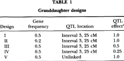
TABLE 1

Granddaughter designs

Gene QTL Design frequency QTL location effect"

I 0.5 Interval 3, 25 cM 1

.o

I1 0.2 Interval 3 , 2 5 cM 1

.o

111 0.5 Interval 3, 25 cM 0.5

Iv 0.5 Interval 3, 25 cM 0.25

V 0.5 Unlinked 1

.o

a In genetic standard deviations.

relative to Monte Carlo standard errors. The starting position for the QTL was always nonlinkage (L = 0 ) . Starting values for MG genotypes and polygenic effects were obtained by first sampling sires and final offspring (sons) jointly by ignoring pedigree information on sires and then sampling the paternal ancestors conditional on offspring genotypes but ignoring parental genotypes, such that offspring preceded parents in a sampling scheme.

Diagnostics from Gibbs output: The Gibbs sampler was run with a burn-in period of 2000 cycles and a length of 100,000 cycles. Autocorrelations for lags from

1 to 5000 were estimated according to GEYER (1992).

An effective sample size (ESS) was computed for each parameter, which estimates the number of independent samples with information content equal to that of the dependent sample of 100,000 (SORENSEN et al. 1995). The analysis of one chromosome with the method as described above (100,000 cycles) took -15 hr CPU on an IBM-SP2 with two Rs/6000 590 processors and eight

RS/6000 390 processors. This length of the sampler yielded ESS of 100 or more for all parameters for designs I and 11. For design 111, 200,000 cycles were required to meet the same minimum ESS.

Marginal posterior probabilities of linkage: Table 2

contains the marginal posterior probabilities of QTL location in each of the intervals and on the flanks based on 100,000 (or 200,000 for design 111) cycles. These probabilities were estimated from Gibbs output by frequency counts of the d , sample values. Summing across intervals yields the probability of the QTL being inside of the linkage group, summing across flanks yields the probability of the QTL being on the flanks, and summing all these probabilities yields the marginal posterior probability of linkage. The prior probability of linkage was set to 20% as in THALLER and HOESCHELE

(1996b).

For designs I and 11, where QTL substitution effect equals one additive genetic SD, the marginal posterior probability of linkage was 100 and 99.9%, respectively. Nonzero probabilities for the flanks resulted only from early cycles following the first 2000 discarded cycles in few replicates. In most replicates, the samples of QTL location were inside the linkage group. In some repli-

TABLE 2

Marginal posterior probabilities of QTL location computed

as Monte Carlo averages of conditional probabilities (10 replicates)

Design"

Interval I I1 I11

Iv

v

0 0.0 0.1 23.9 70.0 84.0

1 5.5 3.2 4.1 11.6 7.1

2 9.0 13.8 30.1 8.6 1.4

3 84.5 80.9 30.7 3.9 2.2

4 0.0 1.8 8.5 2.2 0.8

5 0.0 0.1 1.8 1.8 1.5

6 0.0 0.1 0.9 1.9 3.0

QTL inside linkage group 94.5 96.6 71.1 16.5 5.9 QTL in flanks 5.5 3.3 5.0 13.5 10.1

No linkage 0.0 0.1 23.9 70.0 84.0

Designs are defined in Table 1. Values in

%*loo.

cates, the sampler required several 1000 cycles to move inside the linkage group, which can be considered as additional burn-in. Restarting the sampler once or twice with a different random number seed but with the same starting values lead to a smaller burn-in period. For

designs

I

and I1 the sampler never returned to the flanks

or to nonlinkage once it was inside the linkage group.

For design 111, where QTL substitution effect was half of the additive genetic SD, the marginal posterior probability of linkage was 76.1%. This value still favors linkage given the prior probability of linkage of

20%.

For

design

IV

with substitution effect only equal to one- quarter of the additive genetic SD, the marginal posterior probability of linkage (30%) did not support linkage. For design V representing the null hypothesis of nonlinkage, the marginal posterior probability of linkage was only 16% (less than the prior of 20%). Thus, the linkage hypothesis was clearly rejected.

Parameter estimates: Average parameter estimates (marginal posterior means), their empirical SE due to replications ("empirical SE"), and average SD of the marginal posterior distribution for design I are given in Table 3. Multiplication of the empirical SE by ( yields an estimate of the empirical SE of the individual estimate, which would be identical to the posterior SD

under normality. The QTL parameters were quite well estimated and had sufficiently large ESS. QTL distance was slightly underestimated because in some cycles the QTL was located on the flank (prolonged burn-in for some replicates) or in interval

2

rather than in the correct interval 3, with the true QTL location close to marker 2 separating intervals 2 and 3. If QTL distance was estimated conditional on the QTL being in interval

3, the estimate of d~ was 0.26. The residual and polygenic variances are not well separable with these designs as was also noted by THALLER and HOESCHELE (1996b),

(6)

TABLE 3

Average parameter estimates, standard errors of the average estimates (SE), average posterior standard deviations and effective sample sizes across 10 replicates for design I

True Average Average Effective

Parameter value estimate SE posterior SD sample size

P

0.50 0.54 0.02 0.08

CY 57.50 55.23 1.34 4.49

d e 0.25 0.22 0.03 0.03

0.00 -0.22 1.37 4.13

Od 793.36 704.43 92.84 277.38

U i 860.41 710.56 98.91 271.39

U t 413.44 _511.11 _60.20 _143.18

5

208 505 1039 NC"

156 140 109

Design is defined in Table 1.

" Not computed.

across replicates. For replicates, where QTL distance was sampled almost exclusively in the correct interval, high ESS numbers were found as compared to replicates where QTL distance was sampled in several intervals.

Parameter estimates and related statistics for design

I1 are given in Table

4.

Design I1 differed from I only in the frequency of the favorable QTL allele, which was reduced from 0.5 to 0.2. Again, QTL parameters were quite well estimated, but ESS values were reduced by

-50% for

p

and d, and somewhat less for a. Empirical SE and average posterior SD were higher than those for design I for most parameters.

Table 5 contains the parameter estimates and related statistics for design 111. Design I11 differed from I in the QTL substitution effect, which was halved. Parameter estimates were less accurate than those for design I

and, particularly, gene frequency and gene effect were overestimated. QTL position was significantly underestimated when averaged across all cycles with L = 1, because in 40% of the cases QTL was located in interval

2. However, the estimate was near the true value at 0.27

when conditioned on the QTL being located in interval 3. Empirical SE and average posterior SD were larger than for designs I and 11. ESS of the QTL parameters were <50% of those for design I and slightly less than

those for design I1 with the exception of the much lower ESS number for

a ,

even though Gibbs sample size was increased to 200,000. ESS values of the variance components were almost identical across designs.

For design I the marker distances were very well estimated: 0.20, 0.39, 0.60, and 0.80 for markers

2

to 5 ,

respectively. The empirical SE varied from 0.003 to 0.009 and was higher for those markers being further away from the origin of the linkage group. Average posterior SD ranged from 0,016 to 0.030. Effective sample sizes were -5000. Average estimates of the marker allelic frequencies were virtually identical to the true values. Empirical SE were -0.003 and average posterior

SD -0.009. Effective sample sizes were close to 90,000. These parameters were very well estimated for all designs.

The ranges of the posterior correlations among parameters are presented in Table 6 for designs I and 111.

The highest correlations were those among the variance components. The same result was found by THALLER and HOESCHELE (199613). Correlations of the variance components with the QTL parameters were intermedi- ate to small and variable in sign. Correlations tended to be higher in absolute value for design 111 with the smaller QTL substitution effect. Correlations among the three QTL parameters were very small for design I

TABLE 4

Average parameter estimates, standard errors of the average estimates (SE), average posterior standard deviations and effective sample sizes across 10 replicates for design 11

P

0.80 0.82 0.03 0.06 106

CY 57.50 61.34 1.84 6.16 249

d e 0.25 0.24 0.02 0.09 625

1 -17.25 -18.81 2.09 5.46 NC"

d l 805.41 609.90 119.09 296.41 153

d

z

872.47 620.93 124.06 306.02 156

Ot

562.28 725.74 85.45 160.16 149

Design is defined in Table 1.

(7)

Multiple Marker Linkage Analysis

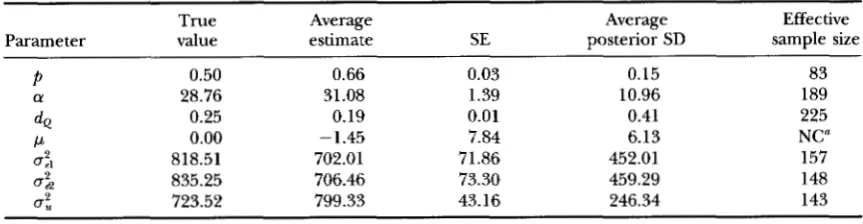
TABLE 5

Average parameter estimates, standard errors of the average estimates (SE), average posterior standard deviations and effective sample sizes across 10 replicates for design III

1837

P

0.50 0.66 0.03 0.15

ff 28.76 31.08 1.39 10.96

d, 0.25 0.19 0.01 0.41

I.1 0.00 -1.45 7.84 6.13

d l 818.51 702.01 71.86 452.01

0: 835.25 706.46 73.30 459.29

0: 723.52 799.33 43.16 246.34

83 189 225 NC"

157 148 143

Design is defined in Table 1. Not computed.

and somewhat more pronounced but very variable in sign for design 111.

Posterior correlations among marker distances de- creased with increasing distance among loci; the highest correlation was 0.86 between markers 4 and 5, and the lowest correlation was 0.44 between markers 2 and 5. The correlation between adjacent marker loci was higher the further the loci were from the origin of

the linkage group. Posterior correlations between the position of the QTL and its adjacent markers were lower (0.41-0.65) than between positions of adjacent markers due to the conditioning on marker order. Posterior correlations between QTL and marker positions de- creased with increasing distance between QTL and marker. For design I11 (smaller a ) correlations between QTL and marker distances were lower than for design I. Posterior correlations among marker allelic frequencies, correlations among frequencies and the other parameters, and correlations among marker distances and the other parameters were all near zero.

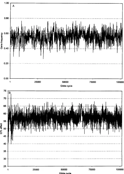
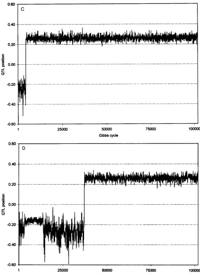
Plots of sample value us. Gibbs cycle can be found in Figure 1 for gene frequency, QTL substitution effect, and QTL position. All plots were obtained from a single replicate for design I. Plots for

p

and a show little or no burn-in. For these parameters, the true parameter values were used as starting values. The plots for the QTL map distance were obtained from the same data set, but the random number sequence was different. The first one is typical for the majority of replicates and

shows a burn-in period ending after a few 1000 cycles, while the other plot depicts the case of a prolonged burn-in. Starting value for QTL position was always nonlinkage. QTL position was subsequently sampled on the flank for some time and then it jumped into intervals 2 and 3 near the true position.

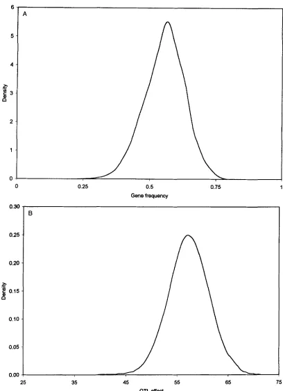
Figure 2 shows marginal posterior density plots for gene frequency, substitution effect, QTL position, and polygenic variance. The marginal density estimates for parameters a ,

p,

and 02, were obtained as averages of

the densities of the conditional sampling distributions that were standard. Parameter d, could not be sampled from a standard distribution, and its marginal density was estimated using the technique of average shifted histograms (SCOTT 1992). Posteriors for a ,

p,

and d, are nearly symmetric and indicate that there was sufficient information in the data to estimate these parameters quite well. The marginal posterior distribution for polygenic variance was skewed, which is consistent with the fact that variance components are not well estimated in these designs.

Alternative sampling schemes: All results reported above were computed with the Gibbs sampler including distances of rather than recombination rates among loci and sampling distances via Metropolis-Hastings. With grid sampling in place of MH, very similar parameter estimates were obtained, and computing time was reduced by 20-30%.

The sampler including recombination rates was

TABLE 6

b g e S of the posterior correlations among parameters evaluated from Gibbs output (across 10 replicates)

P

a d, d l a:

d

P

-0.15, 0.14 -0.10, 0.00 -0.30, 0.06 -0.32, -0.03 0.06, 0.37

a -0.12, 0.59 -0.02, 0.16 -0.37, 0.02 -0.37, -0.02 -0.29, 0.13

d l -0.48, 0.22 -0.37, 0.50 -0.37, 0.24 0.59, 0.81 -0.89, -0.74

d

2

-0.47, 0.23 -0.38, 0.50 -0.37, 0.25 0.95, 0.99 -0.89, -0.76

02, -0.27, 0.48 -0.36, 0.35 -0.41, 0.22 -0.97, -0.86 -0.97, -0.86

d, -0.41, 0.29 -0.70, 0.30 -0.18, 0.04 -0.19, 0.05 -0.08, 0.19

(8)

1838 _P._Uimari,_G._{Thaller and}_I._Hoeschele

1 .oo

A

1

8 0.60

C 0

.k

8

0.40

8-

0 C

25000 soooo

Gibbs cycle

75000 1OOOOO

r

L" r

1 25000 m o o 75000

Gibbs cycle

I

o

m

FIGURE 1.-Sample value us. Gibbs cycle for QTL gene frequency (A), substitution effect (B), and QTL map distance ( C and

D; two different Gibbs runs) for design I.

found not to be competitive in terms of CPU time. butions, eliminating the need for Metropolis-Hastings There was no change in the autocorrelation structure within Gibbs, CPU time per Gibbs cycle was increased that would considerably reduce Gibbs sample size, in due to the augmentation of the MG space, i.e., an in- particular because the variance components exhibited crease in the number of possible genotypes to sample the least favorable autocorrelations. Although the re- from.

(9)

Multiple Marker Linkage Analysis 1839

0.60 1 1

I C

1 25000 50000 75000

G i b s cycle

FIGURE 1.

-

Continued

1OOOOO

QTL using multiple linked markers allowing to investi- accounts for uncertainty about all other parameters. In gate one chromosome at a time for the presence of a ML interval mapping, parameters are estimated condi- single QTL. For each chromosome, the posterior proba- tional on the most likely QTL position, while in the bility of linkage is computed and used to decide _{present method, uncertainty about QTL presence and} whether a QTL is present. The marginal posterior mean location is taken into consideration.

(10)

1840 _P.Uimari, G. Thaller and I. Hoeschele

6

5

4

.-

0

n

5 3

2

1

0 0

0.30

0.25

0.20

3

5

0.15

n

0.10

0.05

0.00

A

0.25 0.5

Gene frequency

0.75

25 35 45 55

QTL effect

65 75

FIGURE 2.-Marginal posterior density of QTL gene frequency (A), substitution effect (B), QTL map distance (C), and polygenic variance (D) from design I.

tiple

QTL,

the utilization of phenotypes on multiple versible jump MCMC” algorithm of GREEN (1995). Fur-

(11)

Multiple Marker Linkage Analysis 1841

10

9

8

7

6

.-

b

i 5

4

3

2

I

C

0.1

0.14 0.18 0.22 0.26 0.3 0.34 0.38

QTL position

0.10

0.08

0.06 .- b

C u)

5

0.04

0.02

0.00

0 250 125 375 625 500 750 875 lo00

Polygenic variance

FIGURE 2.

-

Continued

Compared with the single marker method of particular for the QTL parameters, and when the larger

(12)

1842 P. Uimari, G . Thaller and I. Hoeschele

marker study, a QTL substitution effect of half of the additive genetic SD appears to be near the lower limit for a detectable QTL effect.

The method presented here should be employed to reanalyze interesting regions of the genome identified with an ad hoc method. An initial analysis with a compu- tationally simple method such as linear regression cannot provide estimates of the QTL parameters nor utilize full pedigree information, but allows the investigator to compute exact threshold values for testing a linkage hypothesis via data permutation (CHURCHILL and

DOERGE 1994). Bayesian linkage analysis is also applied in plant genetics (SATAGOPAN et al. 1996) and human genetics (THOMAS and CORTESSIS 1992). The work of these authors has been extended here to continuous phenotypes, more complex models of phenotypic variation, and outcross populations.

The National Science Foundation provided generous support for this project (grant no. BIR-9596247). G.T. acknowledges financial support from the Deutsche Forschnngsgemeinschaft in the form of a postdoctoral fellowship. I.H. acknowledges financial support from the European Human Capital and Mobility Fund while on research leave at Wageningen University, The Netherlands. This research was conducted using the resources of the Cornell Theory Center, which receives major funding from the National Science Foundation and New York State. Additional funding comes from the Advanced Re- search Projects Agency, The National Institutes of Health, IBM Cor- poration, and other members of the center’s Corporate Research Institute.

LITERATURE CITED

ALBERT, J. H., and S. CHIB, 1994 Bayesian model checking for binary and categorical response data. Technical Report, Department of Mathematics and Statistics, Bowling Green University, OH.

CARLIN, J. B., 1992 Meta-analysis for 2x2 tables: a Bayesian approach. Stat. Med. 11: 141-159.

C A R L I N , B. P., and S. CHIB, 1995 Bayesian model choice via Markov chain Monte Carlo methods. J. R. Stat. SOC. Ser. B 57: 473-484. CARLIN, B. P., and N. G. POLSON, 1991 Inference for nonconjugate

Bayesian models using the Gibbs sampler. Can. J. Stat. 19: 399- 405.

CHm, S., and E. CREENBERG, 1995 Understanding the Metropolis- Hastings algorithm. Am. Stat. 49: 327-335.

CHURCHILL, G., and R. DOERGE, 1994 Empirical threshold values for quantitative trait mapping. Genetics 138: 963-971.

DEVROE, L., 1986 N o n u n f m Random Variate Generation. Springer- Verlag Inc., New York.

GELMAN, A,, and D. B. RUBIN, 1992 Inference from iterative simulation using multiple sequences (with discussion), pp. 457-511 in Bayesian Statistics 4, edited by J. M. BERNARDO, J. 0. BERGER, A. P. DAWID and A. F. M. SMITH. Clarendon Press, Oxford.

GEORGE, E. I., and R. E. MCCULLOCH, 1993 Variable selection via Gibbs sampling. J. Am. Stat. Assoc. 88: 881-889.

GEYER, C. J., 1992 Practical Markov chain Monte Carlo (with discus sion). Stat. Sci. 7: 467-511.

GILKS, W. R., and P. WILD, 1992 Adaptive rejection sampling for Gibbs sampling. Appl. Stat. 41: 337-348.

GILKS, W. R., N. G. BEST and K K C. TAN, 1995 Adaptive rejection Metropolis sampling within Gibbs sampling. Appl. Stat. 44: 455- 472.

GODDARD, M., 1992 A mixed model for analyses of data on multiple genetic markers. Theor. Appl. Genet. 83: 878-886.

GREEN, P. J., 1995 Reversiblejump Markov chain Monte Carlo com- putation and Bayesian model determination. Biometrika 82:

711-732.

GUO, S. W., and E. A. THOMPSON, 1992 A monte carlo method for combined segregation and linkage analysis. Am. J. Hum. Genet.

51: 1111-1126.

HOBERT, J. P., and G. CASELLA, 1994 Gibbs sampling with improper prior distributions. Technical Report BU-1221-M, Biometrics Unit, Cornel1 University, Ithaca, N Y .

HOESCHELE, I., and P. M. V A N ~ D E N , 1993a Bayesian analysis of linkage between genetic markers and quantitative trait loci. I. Prior knowledge. Theor. Appl. Genet. 8 5 953-960.

HOESCHELE, I., and P. M. VANRADEN, l993b Bayesian analysis of linkage between genetic markers and quantitative trait loci. II. Combining prior knowledge with experimental evidence. Theor. Appl. Genet. 8 5 946-952.

JANSS, L. L. G., R. THOMPSON and J. A. M. VAN ARENDONK, 1995 Application of Gibbs sampling in a mixed major gene-polygenic inheritance model in animal populations. Theor. Appl. Genet. 91: 1137-1147.

KNOIT, S. A,, and C. S. HALEY, 1992 Aspects of maximum likelihood methods for the mapping of quantitative trait loci in line crosses. Genet. Res. Camb. 60: 139-151.

KUO, L., and B. MALLICK, 1995 Variable selection for regression models. Technical Report, Department of Statistics, University of Connecticut.

MENG, X.-L., and W. H. WONC, 1993 Simulating ratios of normaliz- ing constants via a simple identity: a theoretical exploration. Technical Report No. 365, Department of Statistics, The Univer- sity of Chicago, Chicago, IL.

NEWTON, M. A,, and A. E. RAFTERY 1994 Approximate Bayesian in-

ference with the weighted likelihood bootstrap. J. R. Statist. SOC. Ser. B 56: 3-48.

SATAGOPAN, J. M., B. S. YANDELL, M. A. NEWTON and T. C. OsBOrw, 1996 Markov chain Monte Carlo approach to detect polygene loci for complex traits. Genetics (in press).

SCOTT, W. D., 1992 Multivariate Density Estimation. Wiley and Sons, New York.

SORENSEN, D. A,, S. ANDERSEN, D. GIANOLA and 1. KORSGAARD, 1995 Bayesian inference in threshold models using Gibbs sampling. Genet. Sel. Evol. 27: 229-249.

STEPHENS, D. A., and A. F. M. SMITH, 1993 Bayesian inference in multipoint gene mapping. Ann. Hum. Genet. 57: 65-82. TANNER, M. A., and W. H. WONG, 1987 The calculation of posterior

distributions by data augmentation. J. Amer. Statist. A~SOC. 82:

528-540.

THALLER, G., and I. HOESCHELE, 1996a A Monte Carlo method for Bayesian analysis of linkage between single markers and quantitative trait loci: 1. Methodology. Theor. Appl. Genet. (in press). THALLER, G., and I. HOESCHELE, 1996b A Monte Carlo method for

Bayesian analysis of linkage between single markers and quantitative trait loci: 11. A simulation study. Theor. Appl. Genet. (in

THOMAS, D. C., and V. CORTESSIS, 1992 A Gibbs sampling approach press).

to linkage analysis. Hum. Hered. 42: 63-76.

TIERNEY, L., 1994 Markov chains for exploring posterior distribn- tions (with discussion). Ann. Stat. 22: 1701-1762.

VANRADEN, P. M., and G. R. WIGCANS, 1991 Derivation, calculation and use of national animal model information. J. Dairy Sci. 74:

WAKEFIELD, J. C., A. E. GELFAND and A. F. M. SMITH, 1991 Efficient generation of random variates via the ratio-of-uniforms method.

WANG, C. S., J. J. RUTLEDGE and D. GIANOLA, 1993 Marginal infer- Stat. Comput. 1: 129-133.

ences about variance components in a mixed linear model using Gibbs sampling. Genet. Sel. Evol. 25: 41-62.

WELLER, J. I., Y. KAsHl and M. SOLLER, 1990 Power of daughter and granddaughter designs for determining linkage between marker loci and quantitative trait loci in dairy cattle. J. Dairy Sci. 73:

2737-2746.

2525-2537.