Bayesian Multiple Quantitative Trait Loci Mapping for Complex Traits Using Markers of the Entire Genome

DOI: 10.1534/genetics.106.064980

Bayesian Multiple Quantitative Trait Loci Mapping for Complex

Traits Using Markers of the Entire Genome

Hanwen Huang,* Chevonne D. Eversley,

†

_{David W. Threadgill}

†,‡

_{and Fei Zou*}

,‡,1

*Department of Biostatistics,†Department of Genetics and‡Carolina Center for Genome Sciences,

University of North Carolina, Chapel Hill, North Carolina 27599

Manuscript received August 17, 2006 Accepted for publication April 28, 2007

ABSTRACT

A Bayesian methodology has been developed for multiple quantitative trait loci (QTL) mapping of complex binary traits that follow liability threshold models. Unlike most QTL mapping methods where only one or a few markers are used at a time, the proposed method utilizes all markers across the genome simultaneously. The outperformance of our Bayesian method over the traditional single-marker analysis and interval mapping has been illustrated via simulations and real data analysis to identify candidate loci associated with colorectal cancer.

T

REMENDOUS advances have been achieved over the last decade in the identification of genes un-derlying many heritable traits with the greatest progress limited almost entirely to those with Mendelian inher-itance patterns and well-defined quantitative traits that have relatively large and consistent effects. However, many common pathologies afflicting the greatest num-ber of individuals are not due to simple Mendelian traits. Recent emphasis has been shifted to map com-plex traits, which are caused by the sum of a comcom-plex interaction between gene products and environmental stimuli. Complicating the analysis of these types of traits is the prediction that many are also controlled by genes that have small effects individually, but whose cumula-tive action is the cause of significant interindividual variation. Due to the complex and often subtle nature of phenotypic variation, traits with complex etiologies have proven far more resistant to genetic analysis. Most of the available quantitative trait loci (QTL) mapping methods map only one or a few QTL at a time and therefore are not efficient for mapping such complex traits. Forward and stepwise selection procedures have been proposed in searching for multiple QTL. Though simple, these methods have their limitations, such as the uncertainty of number of QTL, the sequential model building that makes it unclear how to assess the significance of the associated tests, etc.

To overcome this problem, Bayesian QTL mapping (Satagopan et al. 1996; Sillanpaa and Arjas 1998;

Stephens and Fisch 1998; Yi and Xu 2000, 2001;

Hoeschele 2001) has been developed, in particular,

for detection of multiple QTL by treating the number of

QTL as a random variable and specifically modeling it using reversible-jump Markov chain Monte Carlo (MCMC) (Green 1995). Due to the change of dimensionality,

care must be taken in determining the acceptance prob-ability for such a dimension change, which in practice may not be handled correctly (Ven2004). To avoid such

a problem by the uncertain dimensionality of parameter space, Yi (2004) and Xu (2003) proposed a unified

Bayesian framework to identify multiple QTL using all markers across the genome. The method of Xu(2003)

is based on a shrinkage idea to simultaneously evaluate marker effects of the entire genome under the random regression model by assigning each marker a normal prior with mean 0 and an effect-specific variance. The effect-specific prior variance was further assigned a vague prior such that the variance was estimated from the data. Those markers that have no effect on the trait will be essentially shrunk down to 0. Similarly, Yi(2004)

adapted the stochastic search variable selection (SSVS) approach of George and McCulloch (1993) to the

QTL mapping framework. SSVS is a variable selection method that keeps all possible variables in the model and limits the posterior distribution of nonsignificant variables in a small neighborhood of 0 and therefore eliminates the need to remove nonsignificant variables from the model. In principle, Xu(2003) and Yi(2004)’s

methods are similar and both have the ability to control the genetic variances of a large number of QTL where each has small effect (Wanget al. 2005). Due to the

simplicity of Xu(2003), we decide to go with the unified

shrinkage method in this article.

Some quantitative traits do not have continuous mea-surements, but rather are qualitative traits with, for ex-ample, binary measurements. This research is mainly motivated by a colorectal cancer susceptibility study. One hundred thirty-five backcross mice of A/J3SPRET/EiJ F1 1_{Corresponding author:Department of Biostatistics, University of North}

Carolina, 3107D McGavran-Greenberg Hall, CB 7420, Chapel Hill, NC 27599. E-mail: [email protected]

(ASP F1) hybrids to A/J were given intraperitoneal in-jections of the alkylating carcinogen azoxymethane where40% of the mice developed tumors. The goal of the study was to identify susceptibility genes for colo-rectal cancer. Mapping genes for such binary traits is more complicated than that for continuous traits as cur-rent QTL mapping methods are mainly limited to test association between a marker and a binary trait with simple chi-square tests. As an alternative, Hackettand

Weller(1995), Xuand Atchley(1996), and Visscher et al. (1996) proposed interval mapping procedures for complex binary disease traits assuming that the binary traits are controlled by an underlying normally distrib-uted liability. The quantitative liability is then modeled by the usual quantitative genetics model. Due to the apparent success of the unified Bayesian framework to identify multiple QTL using all markers across the ge-nome for normally distributed quantitative traits, the systematic investigation of the unified Bayesian map-ping for complex binary traits would be interesting and useful. In this article, we propose the Bayesian method-ology in mapping complex binary traits and investigate its performance via extensive simulations. Detailed con-vergence diagnostics are also presented.

STATISTICAL METHODS

The liability and threshold model: In the liability model (Wright 1934a,b; Falconer 1965; Falconer

and Mackay1996), a binary trait is assumed to be

con-trolled by a latent liability variable, which is normally distributed. That is, supposediandyi(i¼1,. . .,n) are the binary phenotype and the underlying liability, respec-tively, of theith individual; then the threshold model assumes that there is a fixed threshold in the scale of liability,t, which determinesdi. Specifically,di¼1, ifyi.t; otherwisedi¼0.

Marker analysis:Here we allow only QTL to be located on markers. An extension to allow QTL to be located between markers is discussed in the following section.

For backcross QTL data, we can describe the liabilityyi by the following linear model,

yi ¼m1

XK

j¼1

xijaj1ei; ð1Þ

whereKis the total number of markers;mis the overall population mean,xijis a dummy variable indicating the genotype of thejth marker of individualiwithxij¼1 or 0 if the marker genotype is homozygote or heterozygote, respectively,ajis the partial regression coefficient, andei is the residual error with a distribution of Nð0;s2

eÞ. Note,ajdescribes the genetic effect of the jth marker that partly absorbs the effects of all QTL located be-tween markersj1 andj11, as shown by Zeng(1993).

Similarly, for an F2population, the liabilityyican be related to QTL as

yi¼m1

XK

j¼1

xijaj1

XK

j¼1

wijbj1ei; ð2Þ

wherexijandwijare defined asxij ¼

ffiffiffi

2

p

andwij¼ 1 for genotypeAA,xij¼0 andwij¼1 forAa, andxij¼

ffiffiffi

2

p

andwij¼ 1 foraawithAA,Aa, andaareferring to the three marker genotypes at each locus;ajandbjare the additive and dominance effects of thejth marker; andm andeiare defined the same as in the backcross model.

Since the latent liabilityyis unobserved, the meanm and residual variances2

ecan be set arbitrarily. For model identifiability, we sett¼0 andse¼1 throughout the presentation.

To employ the frequentist method via a likelihood function requires calculation of the conditional proba-bility,pi, ofdi¼1 given {xij,j¼1, 2,. . .,K}, which can be approximated by the logistic model

pi

expðcj_iÞ

11expðcj_iÞ ð3Þ

(Xu and Atchley1996), with j

i ¼m1

PK

j¼1xijaj for the backcross, j_i ¼m1PK_j¼1xijaj1

PK

j¼1wijbj for the F2, andc ¼p=pffiffiffi3. Therefore the log likelihood can be approximated as

L¼X

n

i¼1

dilogðpiÞ1

Xn

i¼1

ð1diÞlogð1piÞ; ð4Þ

where pi is defined above. The maximum-likelihood estimators (MLE) can be obtained by directly maximiz-ingL. However, in practice, the number of markers is often comparable to or even larger than the number of observations. Under such circumstances, the maximum-likelihood method will have very low efficiency or even fail.

Below we describe the Bayesian method which over-comes such a problem. We describe here only the basis for the backcross population. With a minor modifica-tion, it can be easily extended to an F2design.

Bayesian modeling: In the Bayesian framework, both the data and the parameters are treated as random, with random variables being classified as observed and unob-served. The goal of Bayesian analysis is to combine the prior distribution of the unobserved variables with the observed data to obtain a posterior distribution of the un-known variables. The observed data in our QTL setup are the binary responses S¼ fdig

n

i¼1, and the marker genotypesX¼{xij}, fori¼1, 2,. . .,nandj¼1, 2,. . .,K. Our unobserved variables are the liability Y¼ fyigni¼1, the regression coefficients, B¼ m;fajgKj¼1

, and the

variances associated withB;V¼ fs2 jg

K j¼1.

By Bayes’ theorem, the joint posterior density of the parameters {Y,B,V}, given the observed data {S,X}, is

pðY;B;VjS;XÞ

Inference is performed conditional onXand we suppress this conditioning notation for the remainder of the article. We assume that the joint prior distribution ofp(B,V) is

pðB;VÞ ¼pðmÞY K

j¼1

pðajÞ

YK

j¼1

pðs2

jÞ: ð6Þ

Specifically, we choose pðmÞ 1;pðajjs2jÞ ¼fðaj;s2jÞ, andpðs2

jÞ 1=s 2

j, wheref(x,s

2_{) is the density function}

of normal distribution with mean zero and variances2_. The first term in (5) is the conditional distribution of the data given all the unknowns, which equals

pðSjY;B;VÞ

¼Y

n

i¼1

pðdijyiÞ

¼Y

n

i¼1

fIðyi.0ÞIðdi¼1Þ1Iðyi,0ÞIðdi ¼0Þg; ð7Þ

whereI(A) is an indicator function, taking the value of 1 if conditionAis true and 0 otherwise. Note thatp(SjY,

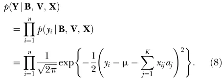
B,V)¼ p(S j Y) because Sdepends solely on Y. The second term in (5) is the conditional distribution of the liability. Because the liability is normally distributed and independent of each other given other variables, we have

pðYjB;V;XÞ

¼Y

n

i¼1

pðyijB;V;XÞ

¼Y

n

i¼1 1

ffiffiffiffiffiffi

2p

p exp 1

2 yim

XK

j¼1

xijaj

!2

( )

: ð8Þ

A MCMC method is used to generate the joint posterior distribution of all unknowns given in (5). Letc¼{Y,B,V} be the collection of unknown variables. For a givenj, if the conditional distribution ofcjgiven the rest of variables has a known standard density, newc_j are drawn via Gibbs samples. Otherwise, we use the Metropolis–Hastings algorithm to draw a new samplec

j according to a proposed density qðc_j;c_jÞ. c_j will be accepted with probability min(1,r), where

r ¼pðc

jjt;cjÞqðc j;cjÞ

pðc_jjt;c_jÞqðc_j;c_jÞ: ð9Þ

Here a negative subscript (j) denotes a vector with the

jth element removed.

We first initializecas follows. The overall meanmand the genetic effects of all QTLfajgKj¼1are initialized with zero while the variances fs2

jg K

j¼1 are initialized with 1. Given the initial values of (B,V), we generateyifrom the corresponding truncated normal distributions,

pðyijB;di ¼1Þ ¼

fðyiji;1Þ

Fðj_iÞ Iðyi.0Þ; ð10Þ

pðyijB;di¼0Þ ¼

fðyiji;1Þ

1Fðj_iÞ Iðyi#0Þ; ð11Þ

where F(x) is the standardized normal distribution function. We describe below the steps for a single MCMC iterative sweept11. Superscripts (t) signify the current variables, and we begin with the initialized values fort¼0:

Step 1. Updating m: m(t11) _{is drawn from the}

poste-rior normal distribution with meanð1=nÞPn i¼1 y

ðtÞ

i

PK

j¼1xija

ðtÞ

j

and variance 1/n.

Step 2. Updatingajforj¼1,. . .,K:a

ðt11Þ

j is drawn from the posterior normal distribution with mean

Xn

i¼1

x_ij21 1

s2_jðtÞ !1_Xn

i¼1

xij y ðtÞ

i mðt11Þ X

l,j

xila ðt11Þ

l

X

l.j

xila ðtÞ l

!

ð12Þ

and variance

Xn

i¼1

x_ij21 1

s2_jðtÞ

!1

: ð13Þ

Step 3. Updatings2

j forj¼1,. . .,K:s 2ðt11Þ

j is sampled from a scale-inverted x2_{-distribution, a}2ðt11Þ

j =x21, wherex2

1is ax

2_{-distribution with 1 d.f.}

Step 4. Updatingyifori¼1,. . .,n:y

ðt11Þ

i is drawn from a truncated normal distribution (10) ifdi¼1 or (11) if

di¼0.

After this round of sampling, we have completed one sweep of the MCMC and are ready to continue our sampling for the next round by repeating steps 1–4 with the newc. When the chain converges, the sampled pa-rameters approximately follow the joint posterior dis-tribution. From the joint posterior sample, one can easily obtain the desired Bayesian estimates, such as the posterior means and variances.

Simulations and real data analysis:The performance of the proposed Bayesian method is evaluated by analyzing a set of simulated backcross data.

A single chromosome with a length of 15 morgans is simulated. On this chromosome, 301 evenly spaced markers (300 intervals, each 5 cM long) are located and two sets of QTL are simulated. In the first setup, four QTL are put along the genome with positions and effects listed in Table 1. Here the QTL are only loosely linked and each QTL explains 20% of the total liability variance. To investigate the ability of the method to identify small QTL effects and to separate closely linked QTL, 11 QTL are evenly placed on the first half of the chromosome,

liability variance explained by the 11 QTL isH¼89.12%. To demonstrate the advantages of the proposed method over the traditional regression method, we simulate 300 individuals, which is smaller than the number of mark-ers; traditional regression analysis fails if all markers are included as covariates. Further, we have simulated 500 individuals to see how sample size affects QTL mapping. For each simulated datum, the sampled parameter values from the first 50,000 sweeps of the chain (burn-in period) were discarded from the analysis. Then we per-formed an additional 500,000 MCMC sweeps. After the burn in, the final sample of observations was selected every 50 sweeps to reduce serial correlation, resulting in 10,000 samples from the posterior.

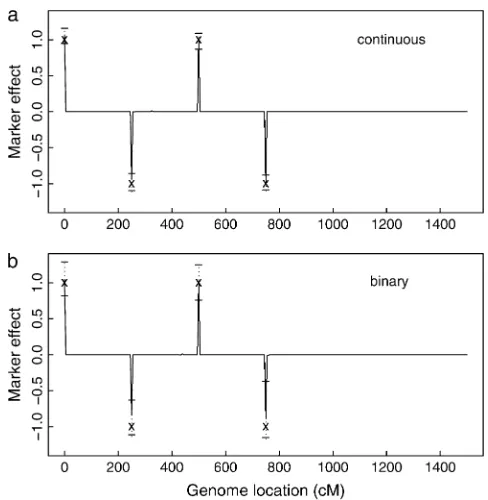
Table 1 shows some summary statistics and Figure 1 shows the estimated QTL-effect profiles (the posterior means of the marker effects) against marker positions along the genome for normal data (Figure 1a) and binary data (Figure 1b) from 10,000 sample states under setup one with sample size 300.

Both profiles show clear signals of QTL at the simu-lated positions. In most cases the estimated QTL effects are close to the true values (Table 1). However, the anal-ysis based on the binary data has reduced efficiency relative to the analysis on the normal liability data di-rectly. This is expected because of the reduced informa-tion in binary data. The histograms of the posterior distribution are also presented in Figure 2. The poste-rior distributions are nearly normal shaped.

The results for setup two where some QTL are closely linked (sample size¼300) are presented in Figure 3. For comparison, we also perform a simple chi-square test at each marker. From Figure 3a, wherelog10(P-value) of the single-marker analysis is plotted, we see many markers that are significantly associated with the simu-lated trait. Because the single-marker analysis fit only one marker at a time, those markers that are correlated with the simulated QTL will also be highly associated

with the trait. On the other hand, in the Bayesian analysis result (Figure 3b), five large QTL are quite clear and four of them are located at the simulated positions with effects also close to the true values. To improve the estimate power, we simulated 500 backcross individuals on the basis of the same setup as above and applied both single-marker and Bayesian analyses on them. The re-sults are depicted in Figure 4. Clearly, the mapping efficiency has been improved quite a lot when sample size increases from 300 to 500 (Figure 4b), where six clear QTL are given at the true positions with effects very close to true values. The smallest QTL that the Bayesian method can pick up in this example explains 2.72% of the liability variance.

Real data analysis:Azoxymethane (AOM) is an alkylat-ing carcinogen that causes strain-specific susceptibility to the development of colorectal tumors in mice. Sus-ceptible mice strains treated with AOM exhibit genetic and pathologic changes similar to those in nonfamilial or sporadic human colorectal cancer. We previously characterized 32 inbred mouse strains for their sus-ceptibility to AOM-induced colorectal tumors and iden-tified the A/J strain as having one of the highest sensitivities, with nearly 100% of mice developing co-lorectal tumors (our unpublished results). In contrast, the genetically distinct strain from the related Mus spretusspecies, SPRET/EiJ, was found to be completely resistant.

Figure1.—Bayesian estimates of QTL effects in the

simu-lated backcross family under setup one. (a) Results from (un-derlying) normal liability data and (b) results from binary data. ‘‘x’’ refers to the simulated QTL position (x-axis) and ef-fect (y-axis). The 95% confidence interval is bracketed by two horizontal lines. The heights of the solid lines correspond to the posterior means.

TABLE 1

QTL parameters and their estimates obtained from the simulated data

QTL

no. Position True effect

Estimated

effect SD P5 P95

1 0 1 1.05 0.14 0.82 1.29

(1.06) (0.06) (0.95) (1.16) 2 250 1 0.87 0.15 1.12 0.63

(0.98) (0.07) (1.10) (0.86) 3 500 1 1.00 0.15 0.76 1.25

(0.98) (0.07) (0.87) (1.09) 4 750 1 0.87 0.24 1.16 0.37

For the current study, we set up a backcross of ASP F1 hybrids to A/J to generate backcross progeny. Two- to 3-month-old mice were given intraperitoneal injections of AOM at 10 mg/kg of body weight once a week for 4 weeks. Subsequently, mice were killed by carbon dioxide asphyxiation 20 weeks after the last AOM dose. A tail clip, a liver sample, and the colon were dissected from each mouse. Each colon was gently flushed with phos-phate buffer saline solution and cut open along its longitudinal axis. The position and size of tumors were recorded before excising any colon tumors for histo-logical verification. Tails, livers, and colons were then placed into labeled Eppendorf tubes and stored at80°. DNA was isolated from liver or tail samples from each mouse by phenol-chloroform extraction. One hundred thirty-five backcross mice were genotyped using the Illumina SNP genotyping platform. Two hundred fifty-four informative markers were used that distinguished the A/J strain from the SPRET/EiJ strain. ASP F1mice were found to be nearly tumor free with5% of mice developing a single colorectal tumor. Analysis of the 135 mice in the backcross population revealed that 40%

of mice developed AOM-induced colorectal tumors (Figure 5).

Since 5% of ASP F1mice still developed a single colorectal tumor, we recategorized the backcross ani-mals into two groups, with one group being tumor free or having a single tumor while the second group was backcross mice developing more than one tumor. The analysis was based on this recategorized binary trait and is summarized in Figure 6. Due to the small sample size, no significant results were identified. However, one re-gion on chromosome 6 is promising. This rere-gion encom-passes a previously detected susceptibility locus for AOM-induced colorectal tumors (Ruivenkamp et al.

2003). We are currently working on collecting another 140 backcross mice to confirm the findings on chromo-some 6. For comparison, the analysis based on a single chi-square test was also performed. Again, the smallestP-value is on chromosome 6, which is consistent with the Bayesian analysis, but it does not survive the genomewide 5% significance level either. Another interesting region indicated by our analysis is located on chromosome 11, which deserves further investigation as well. Figure2.—Histograms for the posterior QTL effects at the four simulated markers for binary data (left) and normal data

Interval mapping:In this section, we extend the QTL mapping on markers to a more general situation where QTL are allowed to be located at any position within marker intervals.

Bayesian modeling: Wang et al. (2005) developed a

method for normal phenotypes that allows a QTL to take a position varying within a marker interval rather than fixed at a marker. They assumed that each marker interval is associated with a QTL, and thus the number of putative QTL is identical to the number of intervals. In their model, the conditional distribution of the QTL genotype given the marker genotypes is derived from a Markov model under the assumption of no segregation inference. The main difference between interval map-ping and marker analysis is that for interval mapmap-ping, the QTL positions and QTL genotypes are unobserved, while for marker analysis, the QTL positions are fixed at markers and also QTL genotypes are observed. A major advantage of the Bayesian analysis is that the unobserved QTL positions and QTL genotypes can be treated as ran-dom variables and sampled via the MCMC procedure. Therefore, for interval mapping, we need only to add ad-ditional steps to the MCMC procedure described above for sampling the QTL positions and QTL genotypes.

For interval mapping, the observed variables are the same as those of the marker analysis, which includeS

and the marker genotypesM¼{mij} (i¼1, 2,. . .,n;j¼1, 2,. . .,K). (Here we change the notation for the marker genotypes from X to M since we reserve X for QTL genotypes. In the marker analysis, the QTL are markers themselves and therefore we refer to marker genotypes asX.) For unobserved variables, besides those in the marker analysis {Y; B; V}, there are additional variables, which include the QTL positions,l¼{lj} forj¼1, 2,. . .,

p; and the QTL genotypesX¼{xij} fori¼1, 2,. . .,nand

j¼1, 2,. . .,p, wherepis the total number of intervals, which in general#K1, and the equality holds only if one chromosome is considered in the analysis.

Now the joint posterior density of the parameters {Y,

l,X,B,V}, given the observed data {S,M}, is

pðY;B;V;l;XjS;MÞ

}pðSjY;B;V;l;X;MÞpðYjB;V;l;X;MÞpðB;V;l;XjMÞ: ð14Þ

Again, inference is performed conditional onMand we suppress this conditioning notation for the remainder of the article.

The last term in (14) is the joint prior, and we assume

pðB;V;l;XÞ

¼pðBÞpðVÞpðXjlÞpðlÞ

¼pðmÞY p

j¼1

pðajÞ

Yp

j¼1

pðs2_jÞY p

j¼1

Yn

i¼1

pðxijjlÞ

Yp

j¼1

pðl_jÞ:

ð15Þ

The prior distributions form,aj, ands2

j are the same as in the marker analysis while for the QTL positions and genotypes, we choose the following prior distributions,

p(lj)¼1/djandxij¼ 1 or 1 with probability1₂each for

i¼1, 2,. . .,n,j¼1, 2,. . .,p, wheredjis the length of the

jth marker interval.

To sample unobserved variables, first we sampleY,B,

Vthe same way as described in steps 1–4 for the marker analysis except that allxij, which are known in the marker analysis, should be replaced byxijðtÞ, samples from thetth iteration. Then the following extra steps are needed to samplel,X:

Step 5. Update QTL genotypes: The QTL genotype

xijðt11Þ(i¼1, 2,. . .,n;j¼1, 2,. . .,p) is updated one Figure3.—Estimates of QTL effects in the

individual and one locus at a time, on the basis of their flanking marker information. Specifically,x_ijðt11Þ

is sampled from the conditional probability distribu-tionp(x), which equals

pðyijx;Bðt11Þ;XðiðtÞjÞÞpðxjm

j iL;m

j iR;l

ðtÞ

j Þ

P

h2f1;11gpðyijx¼h;Bðt11Þ;Xð_iðtÞ_jÞÞpðx¼hjmjiL;m j iR;l

ðtÞ

j Þ

;

wherem_ij_Landm_ij_Rare the two flanking markers of the

jth QTL in the individuali;p xjmijL;m j iR;l

ðtÞ

j

is the

conditional probability of the QTL (at lð_jtÞ) given the two flanking markers;Xð_iðtÞ_jÞ¼ xi1ðt11Þ;. . .;x

ðt11Þ

iðj1Þ;

x_ið_ðtÞ_j11Þ;. . .;x ðtÞ

ip Þand the probability

p yijx;Bðt11Þ;XðitðÞjÞ

}exp 1

2 yim

ðt11Þ_xaðt11Þ

j

Xp

k,j

xikðt11Þa ðt11Þ

k

Xp

k.j

xikðtÞa ðt11Þ k

!2

( )

:ð16Þ

Step 6. Update QTL positions: lð_jt11Þ is sampled via a Metropolis–Hastings approach since there is no closed form for the conditional posterior probability density of a QTL position. We first sample a new positionl

j uniformly from the neighborhood of lð_jtÞ;½lð_jtÞd;

lð_jtÞ1d withd being a tuning parameter, which we take a value of 2 cM in subsequent simulations.l_j will then be accepted or rejected according to the prob-ability min(1,a), where

Figure5.—Number of tumors in two parental

strains A/J and SPRET/EiJ, plus ASP F1and back-cross strains.

Figure_{4.—Estimates of QTL effects in the}

a¼Y n

i¼1

p x _ijðt11Þjmj_iL;mj_iR;l_j

p x _ijðt11Þjmj_iL;mj_iR;lð_jtÞ

qlð_jtÞ

q l_j

: ð17Þ

If neitherlð_jtÞnorl_j is withind-distance away from the ends of the interval, qðl_jÞ ¼qðl_jðtÞÞ ¼1=ð2dÞ. How-ever, iflð_jtÞor/andl_j are withind-distance from one end of the interval, then

qðl_jÞ ¼ 1

d1minðd;t_jÞ;or=andqðl

ðtÞ j Þ ¼

1

d1minðd;tð_jtÞÞ; ð18Þ

wheretð_jtÞis the distance oflð_jtÞfrom the nearest end of the interval; similarly,t

j is the distance ofl

j from the nearest end of the interval.

After these two extra steps for sampling l, X, one MCMC iteration is done and we then continue our sam-pling for the next round by repeating steps 1–6 with the newc.

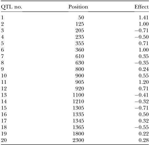
TABLE 2

QTL parameters and their positions

QTL no. Position Effect

1 50 1.41

2 125 1.00

3 205 0.71

4 235 0.50

5 355 0.71

6 360 1.00

7 610 0.35

8 630 0.35

9 800 0.24

10 900 0.55

11 905 1.20

12 920 0.71

13 1100 0.41

14 1210 0.32

15 1305 0.71

16 1335 0.50

17 1345 0.32

18 1365 0.55

19 1800 0.22

20 2300 0.28

Figure7.—Bayesian estimates of QTL effects in the

simu-lated backcross family with four QTL for continuous and bi-nary data. ‘‘x’’ refers the simulated QTL position (x-axis) and effect (y-axis). The 95% confidence interval is bracketed by two horizontal lines. The heights of the solid lines correspond to the posterior means.

Figure6.—(a) Bayesian analysis; (b)

Simulation studies:For interval mapping, a backcross population of 500 individuals was simulated. We in-vestigated a single large chromosome of 24 M that was covered by 121 evenly spaced markers (120 intervals, each 20 cM long). Two sets of QTL are simulated. In the first setup, four QTL are placed at 50, 450, 850, and 1250 cM with effects 1,1, 1, and1, respectively. The sec-ond simulation setups are described in Table 2. Figure 7 shows the estimated QTL effect against QTL positions along the genome for continuous and binary data for setup one. The QTL signals are clearly shown at the simulated positions for both cases. The QTL effects are almost equal to the true values in the normal case but a little larger than the true values in the binary case. Figure 8 presents the QTL positions and effects along with the real positions and effects for continuous and binary data, respectively, for setup two. It is shown that the Bayesian shrinkage method performs better for normal data than for binary data, especially for those QTL that locate in the region beyond 100 cM and have small effects. Parameters of closely linked QTL are hard to estimate. For example, the following QTL pairs, (5, 6), (10, 11), and (16, 17), are so tightly linked that they are inseparable in both normal and binary data cases. QTL 7 and 8, which are closely linked and have the same size but with opposite directions, are not detected in either data set. Nevertheless, for binary data, our method can clearly localize separable QTL and QTL with large effects. A much denser marker set along with a larger

population size is required to resolve QTL with tight linkage and small effect.

Convergence diagnostics tests:Two convergence diag-nostics tests are performed using convergence diagnosis and output analysis (CODA) software (Bestet al. 1995) to

make sure that the sample is representative of the under-lying stationary distribution. The parameters we consider here includemand the effect of four markers at which the true QTL are located. Figure 9 shows the autocorre-lation function against the lag for the setup one simu-lation described in theMarker analysissection, where the number of markers is larger than the number of samples. The autocorrelation appears to be very small after lag 20 for all five parameters. The small autocorrelation shows no indication of slow convergence for the chain. For the same data set, we run five parallel Markov chains with the same length 10,000 using very different initial values to test Gelman and Rubin statistics. Figure 10 shows plots for the 50 and 97.5% quantiles of the sampling distribu-tion for the shrink factor for above five parameters. The plots in Figure 10 show that both the median and the 97.5% quantiles stabilize around the expected value 1.0, indicating that the Markov chains converge to their limiting distribution.

DISCUSSION

The Bayesian method developed in Xu (2003) has

been extended to complex binary traits assuming the

Figure 8.—Bayesian estimates of

threshold model. The results outperform the single-marker chi-square test. The major advantage of using the threshold model is that once the underlying liability is generated, all other unknowns have conditional posterior distributions identical to those already given in the Bayesian analysis of normal data. This methodol-ogy can be easily generalized to multiple-ordered cate-gorical traits. As an alternative to the approach of the liability augmentation, one can directly use the relation-ship (3) between the binary phenotype and the model effects. The problem is that normal is not a conjugate prior to logistic distribution and therefore Gibbs sam-pling will not work in this case. The Metropolis–Hastings algorithm or some complicated sampling scheme like ARMS (Gilksand Wild1992) can be used but it is less

efficient than the Gibbs sampling. The method has been implemented in C and the source codes are available from http://www.bios.unc.edu/_{hhuang/QTLBinary.}

The most striking feature of the Bayesian analysis is that the estimated profiles show clear signal only at a few positions with all remaining markers having effects that are close to zero. This shrinkage effect has been ex-plained in detail in Xu (2003). The key point is that

the priors of the variances of QTL effects are allowed to vary across markers instead of being fixed. This is demonstrated clearly in the special forms of (12) and (13). A large aj will have large variancesjand thus a negligible 1=s2

j, which will lead to a small shrinkage effect. However, if a QTL has a small effect, a smalls2 j will be expected, which will generate a large ratio 1=s2

j and dominate overPn_i¼1x2

ij; thusajwill be very likely shrunk toward zero.

In this article, we have considered the cases that QTL are fixed at the observed markers and that one QTL can be located within each marker interval. For densely distributed markers, the former method is a good ap-proximation to the latter one since the two methods make almost no difference. However, the first method may lead to biased results when the marker density is not high enough. One assumption made in the second method is that each interval contains at most one QTL, which may not be true if two markers are far apart. Yi

(2004) has developed a new method that assumes that, on average, there is at most one QTL in everydcM. The pseudomarkers are introduced to make every interval the same length. The genotypes at pseudomarkers are Figure _{9.—Autocorrelation function for}

the study of setup one. Here b0 represents

treated as missing and can be easily handled in a Bayes-ian framework.

Several frequency-based model selection methods have been developed for mapping multiple QTL. To re-duce modeling space, Carlborgand Andersson(2002)

included only those markers that are significantly asso-ciated with the trait from the single-locus model in the multiple-marker model. Coffmanet al. (2005) first

selected one marker per linkage group, regardless of whether that marker is significantly associated with the trait or not, and then fitted their model on the basis of the chosen markers. Both approaches may identify multiple linked QTL in a biased way as mentioned in Kaoet al. (1999). Our method keeps all possible models

under consideration and therefore avoids potential se-lection bias of the above approaches. Although the vari-able dimension of our model is very high, our Bayesian model is simple and straightforward since standard Gibbs are mainly used in each MCMC iteration. We have tested the method on 300 individuals with 2000 markers and it took less than only 1 hr to generate 100,000 sweeps on a 3-GH linux machine. Convergence

diagnostic tests also show that our method converges quickly and well.

Our method is particularly designed for the situation where no any prior information for the number of QTL and their positions is available. However, it should be noted that the method can be modified to include such prior information. For example, instead of using a noninformative prior fors2

j, we may use different priors for s2

j on the basis of the available information from other studies. For example, if there is strong evidence of a QTL in a region, we may lets2_{’s in the region follow a} uniform prior on½a,bwithabeing large. On the other hand, if there is strong evidence that no such QTL exists in another region, we may then let s2_{’s in this region} follow a uniform prior on ½0,cwithc being small. Of course, introducing such region-specific priors compli-cates the MCMC procedure but would be beneficial especially when the sample size is small.

Further, our model currently can handle only main QTL effects. Another important extension is to include epistatic effects in the model. Several articles (Yiand Xu

2002; Naritaand Sasaki2004) have discussed this issue

Figure 10.—Plot of Gelman and Rubin’s

for normal traits. To include epistatic effects, an upper bound of the number of QTL in the model (Yi_{et al}.

2005) has to be placed, which is extremely useful and necessary since the number of variables dramatically increases when epistatic effects are considered.

Finally, it worth mention that we have run marker analysis only on the real data. We have found that a significantly amount of markers are in segregation dis-tortion, which will affect the genetic map that the in-terval mapping heavily relies on. However, marker analysis is unrelated to the genetic map and therefore is more robust to such segregation distortion. We are currently carefully investigating the causes of such seg-regation distortion, which itself may provide us insights on the etiology of colorectal cancer.

The authors thank the associate editor and two referees for helpful comments and suggestions, which have led to an improvement of this article. This work has been partially supported by National Institutes of Health grants MH070504, GM074175, CA105417, and CA079869.

LITERATURE CITED

Best_{, N. C., M. K. C}owles_{and S. K. V}ines_{, 1995 CODA Manual}

Ver-sion 0.30. MRC Biostatistics Unit, Cambridge, UK.

Carlborg_{, O., and L. A}ndersson_{, 2002 Use of randomization}

test-ing to detect multiple epistatic QTL. Genet. Res.79:175–184.

Coffman_{, C. J., R. W. D}oerge_{, K. L. S}imonsen_{, K. M. N}ichols_{, C. K.}

Duarteet al., 2005 Model selection in binary trait locus

map-ping. Genetics170:1281–1297.

Falconer_{, D. S., 1965 The inheritance of liability to certain diseases,}

estimated from the incidence among relatives. Ann. Hum. Genet.

29:51–71.

Falconer, D. S., and T. F. C. Mackay, 1996 Introduction to

Quantita-tive Genetics, Ed. 4. Addison-Wesley, Boston.

George, E. I., and R. E. McCulloch, 1993 Variable selection via

Gibbs sampling. J. Am. Stat. Assoc.88:881–889.

Gilks, W. R., and P. Wild, 1992 Adaptive rejection sampling for

Gibbs sampling. Appl. Stat.41:337–348.

Green_{, P. J., 1995 Reversible jump Markov chain Monte Carlo}

com-putation and Bayesian model determination. Biometrika 82:

711–732.

Hackett, C. A., and J. I. Weller, 1995 Genetic mapping of

quan-titative trait loci for traits with ordinal distributions. Biometrics

51:1252–1263.

Hoeschele, I., 2001 Mapping quantitative trait loci in outbred

ped-igrees, pp. 599–644 inHandbook of Statistical Genetics, edited by D. J. Balding, M. Bishopand C. Cannings. Wiley, New York.

Kao_{, C. H., Z. B. Z}eng_{and R. D. T}easdale_{, 1999 Multiple interval}

mapping for quantitative trait loci. Genetics152:1203–1216.

Narita_{, A., and Y. S}asaki_{, 2004 Detection of multiple QTL with}

ep-istatic effects under a mixed inheritance model in an outbred population. Genet. Sel. Evol.36:415–433.

Ruivenkamp_{, C. A., T. C}sikos_{, A. M. K}lous_{, T. V. W}ezel_{and P. D}emant_,

2003 Five new mouse susceptibility to colon cancer loci, Scc11-Scc15. Oncogene22:7258–7260.

Satagopan, J. M., B. S. Yandell, M. A. Newtonand T. C. Osborn,

1996 A Bayesian approach to detect quantitative trait loci using Markov chain Monte Carlo. Genetics144:805–816.

Sillanpaa_{, M. J., and E. A}rjas_{, 1998 Bayesian mapping of multiple}

quantitative trait loci from incomplete inbred line cross data. Genetics148:1373–1388.

Stephens, D. A., and R. D. Fisch, 1998 Bayesian analysis of

quanti-tative trait locus data using reversible jump Markov chain Monte Carlo. Biometrics54:1334–1347.

Ven, R. V., 2004 Reversible-jump Markov chain Monte Carlo for

quantitative trait loci mapping. Genetics167:1033–1035.

Visscher, P. M., C. S. Haleyand S. A. Knott, 1996 Mapping QTLs for

binary traits in backcross andF2populations. Genet. Res.68:55–63. Wang, H., Y.-M. Zhang, X. Li, G. L. Masinde, S. Mohan et al.,

2005 Bayesian shrinkage estimation of quantitative trait loci pa-rameters. Genetics170:465–480.

Wright, S., 1934a An analysis of variability in number of digits in an

inbred strain of guinea pigs. Genetics19:506–536.

Wright, S., 1934b The results of crosses between inbred strains of

guinea pigs, differing in number of digits. Genetics19:537–551. Xu, S., 2003 Estimating polygenic effects using markers of the entire

genome. Genetics163:789–810.

Xu, S., and W. R. Atchley, 1996 Mapping quantitative trait loci for

complex binary diseases using line crosses. Genetics143:1417– 1424.

Yi_{, N., 2004 A unified Markov chain Monte Carlo framework for}

mapping multiple quantitative trait loci. Genetics167:967–975. Yi, N., and S. Xu, 2000 Bayesian mapping of quantitative trait loci

for complex binary traits. Genetics155:1391–1403.

Yi, N., and S. Xu, 2001 Bayesian mapping of quantitative trait loci

under complicated mating designs. Genetics157:1759–1771. Yi, N., and S. Xu, 2002 Mapping quantitative trait loci with epistatic

effects. Genet. Res.79:185–198.

Yi, N., B. S. Yandell, G. A. Churchill, D. B. Allison, E. J. Eisenet al.,

2005 Bayesian model selection for genome-wide epistatic quan-titative trait loci analysis. Genetics170:1333–1344.

Zeng, Z. B., 1993 Theoretical basis for separation of multiple linked

gene effects in mapping quantitative trait loci. Proc. Natl. Acad. Sci. USA90:10972–10976.