DOI: 10.1534/genetics.107.071407
A Statistical Framework for Expression Quantitative Trait Loci Mapping
Meng Chen* and Christina Kendziorski
†,1*Pfizer Global Research and Development, Groton, Connecticut 06340 and†Department of Biostatistics and Medical Informatics, University of Wisconsin, Madison, Wisconsin 53706
Manuscript received January 31, 2007 Accepted for publication July 21, 2007
ABSTRACT
In 2001, Sen and Churchill reported a general Bayesian framework for quantitative trait loci (QTL) mapping in inbred line crosses. The framework is a powerful one, as many QTL mapping methods can be represented as special cases and many important considerations are accommodated. These considerations include accounting for covariates, nonstandard crosses, missing genotypes, genotyping errors, multiple in-teracting QTL, and nonnormal as well as multivariate phenotypes. The dimension of a multivariate pheno-type easily handled within the framework is bounded by the number of subjects, as a full-rank covariance matrix describing correlations across the phenotypes is required. We address this limitation and extend the Sen–Churchill framework to accommodate expression quantitative trait loci (eQTL) mapping studies, where high-dimensional gene-expression phenotypes are obtained via microarrays. Doing so allows for the precise comparison of existing eQTL mapping approaches and facilitates the development of an eQTL interval-mapping approach that shares information across transcripts and improves localization of eQTL. Evaluations are based on simulation studies and a study of diabetes in mice.
T
HE quantitative trait loci (QTL) mapping frameworkdeveloped by Senand Churchill(2001), referred
to hereinafter as the Sen–Churchill framework, unifies many methods for QTL mapping in inbred line crosses.
The seminal work of Landerand Botstein(1989) and
subsequent methods including Haley–Knott regression (1992), composite interval mapping, and multiple QTL
mapping ( Jansen1993; Zeng1993, 1994; Jansenand
Stam1994), are all represented, at least approximately,
as special cases of the framework. The framework also accounts for covariates, nonstandard cross designs, miss-ing genotype data, genotypmiss-ing errors, multiple interactmiss-ing QTL, and nonnormal as well as multivariate phenotypes. As a result, it provides a powerful approach to localize the genetic basis of quantitative traits.
There has been much interest recently in identifying the genetic basis of thousands of gene- expression traits
measured via microarrays (Brem et al. 2002; Schadt
et al. 2003; Yvertet al. 2003; Cox2004). The multi-trait version of the Sen–Churchill framework is based on the multivariate normal distribution. This approach becomes problematic when the number of traits is larger than the number of subjects, as the estimated covariance matrix will have less than full rank. To address this, we here extend the Sen–Churchill framework to accommodate expression phenotypes. We first highlight aspects of the Sen–Churchill framework important to our develop-ment, and then detail the extension. We show that the
extended framework generalizes the currently available expression QTL (eQTL) mapping methods and facili-tates the development of an approach that allows for both interval mapping of eQTL and information shar-ing across transcripts. Evaluations are based on simulation studies and a study of diabetes in mice. Generalizations of the framework are also discussed. Many of the
tech-nical details can be found in theappendixes.
A FRAMEWORK FOR EXPRESSION QTL INFERENCE
The Sen–Churchill framework: The Sen–Churchill framework supports a Bayesian approach to QTL map-ping that accommodates a variety of phenotypes and data structures. Much of the flexibility of the approach is due to two main features. The first is marked separa-tion of the genetic model, which relates phenotype to genotype, and the linkage model, which relates putative QTL genotype to the marker map. The second feature is that computation relies on an efficient Monte Carlo component instead of a more complex MCMC pro-cedure as employed in a number of other Bayesian QTL
methods (Satagopan et al. 1996; Yi and Xu 2000; Yi
2004). As we discuss in detail below, these two features allow for accommodation of microarray data as a pheno-type within the framework. We here provide an overview of the framework, focusing on aspects important to our extension.
Suppose that quantitative traits are measured forn
mem-bers of an inbred line cross. Denote the traits by y¼
y1;y2;. . .;yn
ð Þ9 and denote the corresponding marker
1Corresponding author: Department of Biostatistics and Medical
In-formatics, 6729 Medical Sciences Center, 1300 University Ave., Madison, WI 53706. E-mail: [email protected]
data by then3Mmatrixm, whereMdenotes the total number of markers. Marker location and genetic dis-tances are assumed known, although in practice these
are estimated. A genetic modelHdescribes the way in
which QTL genotypes determine a phenotype; it is pre-scribed by the number of QTL, their locations, and the way in which they act and interact to affect the
pheno-type. AssumingpQTL in a genetic model, letgdenote
thep-dimensional vector of QTL locations andgdenote
then3pmatrix of QTL genotypes. The parameters of the
genetic model are denoted bym.
Of primary interest is the posterior distribution of
QTL location,p(gjy,m), given by
pðgjy;mÞ} ð
pðyjgÞpðgjm;gÞpðgÞdg; ð1Þ
where modes ofp(gjy,m) estimate QTL position. An
exact evaluation of Equation 1 is computationally pro-hibitive, but an approximation can be obtained by sam-pling multiple versions of the putative QTL genotypes
gand averaging as follows:
1. Select a regularly spaced gridGof pseudomarker
lo-cations, locations for which genotypes are not known,
and create qrealizations of the pseudomarkers by
sampling fromp(gjm). Assuming known genetic
dis-tances and no crossover interference, a Markov chain sampling scheme can be used. Each realization of
pseudomarker genotypes is ann3Gmatrix.
2. For the assumed genetic modelH, ap-dimensional
vector of pseudomarker locations corresponding to
the QTL, gH, is prescribed; and the ith realization
of pseudomarker genotypes providesgi(gH), ann3
p matrix of pseudomarker genotypes at the QTL
locations.
3. For each realization, calculate a weight under the
as-sumed genetic modelH. The weight for theith
reali-zation is
WHðgiðgHÞÞ ¼pðyjg ¼giðgHÞÞpðg¼gHÞ:
4. An average overqof these weights approximates (1),
according to the principle of importance sampling
pðgHjy;mÞ CX q
i¼1
WHðgiðgHÞÞ
for some constant of proportionalityC.
Extensions to eQTL mapping:Consider for simplicity
a backcross population genotyped asaa(0) orAa(1) atM
markers (this simplification to a backcross is not required
and is relaxed in theApplications to data from a study of
dia-betes). For eQTL mapping, the observed phenotype datay
are no longer a vector as above, but rather aT3nmatrix
of expression levels. Specifically,y¼(y1,y2,. . .,yT)9, where
vector yt ¼ (yt1,. . ., ytn) denotes the (possibly
trans-formed) expression levels for transcripttmeasured inn
animals. As in the univariate phenotype case,mdenotes
ann3Mmatrix containing genotypes onMmarkers.
Of most interest is the identification of significant linkages between transcripts and genome locations. To
be precise, a transcripttis linked to locationlifm0
t;l6¼
m1
t;l where m
0ð1Þ
t;l denotes the latent mean level of
ex-pression for transcriptt for the population of animals
with genotype 0(1) at locationl. TwoT 3 Gmatrices,
u0 and u1, contain the latent mean levels of
expres-sion ðu¼ ðu0;u1ÞÞ
; and, as above, G denotes the total
number of locations considered. In the Sen–Churchill framework, of primary interest is the posterior
evalua-tion ofg, a vector of QTL locations. In this context,gis
transcript specific. For example, for transcript t, gt
would contain indexesl9such thatm0
t;l96¼m1t;l9.
Single eQTL mapping methods:Suppose that a
tran-script is affected by at most one genotype locationl(this
assumption can be relaxed as discussed later) and
con-sider inference at locationl. Of most interest is the
pos-terior probability that transcripttis linked to locationl.
We show inappendix bthat
pðgt¼ljy;mÞ} ð
fP1lðytjgÞpðgjm;gt ¼lÞpðgt¼lÞdg;
ð2Þ
wherefP1l is the marginal density describing the data in
the case of linkage tol.
Equation 2 is similar in form to (1), but there are some important differences. In Equation 2, condition-ing is done on the full set of transcripts. An assumption of conditional independence across transcripts (see appendixes) yields a right-hand side (RHS) that is
eval-uatedonly at the transcript of interestt. The form offP1
determines whether or not information from other
tran-scripts affects the evaluation. For example, iffP1is taken
to be a univariate Gaussian (or other parametric) dis-tribution, then the RHS is completely determined by the
data attsince the parameters offP1do not depend on
other transcripts. An application of the extended Sen– Churchill framework in this case would consist of a re-peated application of a single-transcript analysis to each expression trait in isolation. This has been done in a number of eQTL studies to yield effective results. How-ever, with this approach, there is no information shared across transcripts. As pointed out in a number of articles
on microarray data analysis (Newtonet al. 2001; Tusher
et al. 2001; Kendziorskiet al. 2003; Smyth2004; Cuiet al. 2005), information sharing is important to improve sen-sitivity and moderate test statistics that are otherwise
prone to inflated error. Kendziorskiet al. (2006)
The MOM model is represented as a special case of
the extended framework whenfP1is taken to be a certain
predictive density. In short, assume measurements of
transcripttfor animalr, denotedytr, arise as
condition-ally independent random deviations from an
observa-tion distribuobserva-tionfobs( jm:t,u) with the m
:
t’s as random
effects described by a distributionp(m). The model is
assumed to be the same across locations and so
de-pendence onlis suppressed. In this model, an
equiva-lently expressed transcriptt presents dataytaccording
to the distribution
fP0ðytÞ ¼ ð Yn
r¼1
fobsðytrjmÞ !
pðmÞdm; ð3Þ
wherem¼m0
t ¼m
1
t andfP1ðytÞ ¼fP0(y0t)fP0(y1t) describes
the data for mapping transcripts, owing to the fact that
different mean values,m0
t andm
1
t, govern the different
subsets y0
t and y
1
t of samples and are considered
in-dependent draws fromp(m) (seeappendixes). Here,y0
t
andy1
t denote the collection of expression values from
subjects with genotypes aa and Aa, respectively. As
detailed in Kendziorskiet al. (2006), a Gaussian model
is assumed forfobs() andp(). We also allowed for the
possibility that different clusters of transcripts could pres-ent data with differpres-ent variances.
Specification of the denominatorp(ytjm) of Equation
2 is not required if closed forms for (or good approx-imations of) parameter estimates are available and esti-mation of the false discovery rate (FDR) is not of interest. When closed forms are not available and/or calculation
of estimated FDR is of interest,p(ytjm) must be
eval-uated. Note that pðytjmÞ ¼pðytjm;gt ¼0Þpðgt ¼0Þ1
PG
ll¼1pðytjm;gt ¼llÞpðgt ¼llÞ, wherep(gt¼0) implies
that the transcript does not map to any of theG
loca-tions. We do not assume any specific priors on the mix-ing proportions. They will be estimated usmix-ing the data.
As detailed inappendix b, Equation 2 then becomes
pðgt¼ljy;mÞ
¼
Ð
fP1lðytjgÞpðgjm;gt¼lÞpðgt¼lÞdg fP0ðytÞpðgt¼0Þ1
PG ll¼1
Ð
fll
P1ðytjgÞpðgjm;gt¼llÞpðgt¼llÞdg :
ð4Þ
Note that conditioning on genotype is dropped if the
transcript is not linked to locationlas all measurements
arise from a distribution with common mean and so genotype information, which prescribes groups in the
case of a transcript mapping tol, is not required.
When evaluated at markers only, where genotypes are known, Equation 4 is identical to the MOM model. Extensions of MOM to interval mapping have been difficult to date, as evaluation of Equation 4 can be
prohibitive in between markers. Since thelth column of
g, denotedgl
, is a vector of lengthn, there are 2n
possible genotypes (for a backcross); and as a result, the integral
in Equation 4 is a very large mixture, when n is even
moderately large. In practice, one could potentially re-strict to fewer possibilities since many genotype vectors have very small probabilities. However, as the number of
individuals in the study gets large (.200), this quickly
becomes computationally infeasible even with the re-striction. Fortunately, pseudomarkers can be used, as in the Sen–Churchill framework, to overcome this problem.
In the extended framework, multiple versions of
pseudomarkers are sampled fromp(glj
m). Suppose for
each location l (l ¼1,. . ., G), q genotype vectors are
sampled from the proposal distributionp(gjm) to yield
(gl
1,g2l,. . .,gql). Then Equation 4 is approximated by
pðgt¼ljy;mÞ
pðgt¼lÞ
Pq
i¼1fP1lðytjgilÞ
pðgt¼0ÞPiq¼1fP0ðytÞ1
PG
ll¼1pðgt¼llÞ
Pq
i¼1fP1llðytjgillÞ
ð5Þ
and modes of this distribution are used to estimate eQTL positions. One can apply this approach to grids of
varying sizes (i.e., varyingG) to localize eQTL at and in
between markers. We refer to this approach as pseudo-marker MOM (psMOM).
Simulations:We conducted a small set of simulations to compare psMOM with traditional interval mapping (IM) applied to each transcript in isolation. The simula-tions are not designed to capture the many complexities of eQTL data, but rather they provide some preliminary information on operating characteristics in simple set-tings. Marker genotype data were simulated for four chro-mosomes, each of length 100 cM and having 11 equally spaced markers (10-cM spacing). We assumed that 15% of all transcripts map to at least one genomic location; 5% map to a single location on chromosome 1 (26 cM); 5% map to two locations on chromosome 2 (44 and 56 cM); the remaining 5% map to two locations on chro-mosome 3 (22 and 82 cM). No transcripts are affected by alleles on chromosome 4.
Backcross data were simulated for 200 animals and 4000 transcripts. Simulated intensities follow the
ap-proach described in Kendziorskiet al. (2006). Briefly, we
assume log intensities are normally distributed, which is consistent with the assumptions of both IM and psMOM. Transcript-specific means and variances are sampled from
the empirical means and variances of the F2cross
de-scribed previously. The latent means of transcripts
mapping to a single location satisfym0
t;l6¼m1t;l. For the
transcripts mapping to two locations l¼(l1, l2), their
latent means satisfy mðt0;l;0Þ6¼ m
ð1;0Þ
t;l ¼m
ð0;1Þ
t;l 6¼m
ð1;1Þ
t;l .
Twenty simulated data sets were generated.
Implementation of IM: For IM, we consider fP1 as
psMOM (see below), likelihood ratios (LRs) are derived from the LOD scores, normalized, and converted to quan-tities similar to posterior probabilities. For example, if
L(H1, l9)/L(H0) denotes the likelihood ratio at
loca-tionl9, we considerLðH0Þ= PGl¼1LðH0Þ1LðH1;lÞ
and
LðH1;l9Þ= PG
l¼1LðH0Þ1LðH1;lÞ
as evidence of
equiv-alent and differential expression atl9, respectively. We
refer to these as LOD posterior probabilities. Transcripts with LOD posterior probability of differential expres-sion exceeding some threshold are considered mapping transcripts. As shown in Tables 1–3, IM is evaluated for varying thresholds.
For some examples (noted in subsequent text), to compare with the HPD regions derived from LOD pos-terior probabilities, we also considered 1.5-LOD
drop-support intervals around peak LOD scores (Mangin
et al. 1994; Dupuisand Siegmund1999). They are de-signed to target confidence regions of level 95%, but in general, these intervals are known to be biased in that
they are too small (Visscheret al. 1996). On the other
hand, confidence intervals that are slightly too small favor IM as eQTL appear to be better localized. To give IM the best results, we consider a 10-cM window around the true eQTL positions and define the respective LOD peaks as the highest LODs within the windows. The 1.5-LOD support intervals are then constructed. Of course, in practice, one does not have the luxury of knowing where to choose these peaks and perhaps only the largest peak would be identified. In this way, the results of this approach are further biased in favor of IM.
Implementation of psMOM: Equation 4 is first
eval-uated at the genotyped markers and theM9markers with
posterior probabilities$0.9 define an HPD region. In
particular, the posterior probabilities at the identified
M9markers are averaged across the mapping transcripts
and, using thisM9vector, an HPD region is identified.
Basically, the HPD region contains the minimum num-ber of support points with corresponding posterior
prob-abilities having a sum exceeding 1 –a. More precisely,
the HPD region of level 1a is constructed by rank
ordering posterior probabilitiesp(1)#p(2)#. . .#p(n)
wherePnk¼1pðkÞ¼1 and identifying the largest (n9) such
thatPnk¼n9pðkÞ$1a. The HPD region then consists of
the support points corresponding top(n9),p(n911),. . .,p(n).
A pseudomarker grid is set up within the HPD region and multiple versions of pseudomarkers are gener-ated. The model fit is carried out utilizing all genotyped
markerspluspseudomarkers in the HPD regions. The
procedure provides a matrix of posterior probabilities for every transcript at every test point. As in IM, 500 sets of pseudomarkers are generated every 2 cM; unlike IM, the pseudomarkers are only generated within the HPD
region and thus the dimension of Ghere is reduced,
thereby reducing the computational burden. The pro-cedure gives a matrix of posterior probabilities for every
transcript and every test point. Transcripttis defined to
map to location l if the posterior probability in the
second stage exceeds some threshold. As in IM, psMOM is evaluated for varying thresholds.
Choice of threshold: A list of mapping transcripts
with target FDR acan be constructed by taking those
with posterior probability of equivalent expression less thana(Newtonet al. 2004). This specifies transcripts that likely harbor at least one eQTL, but does not pro-vide information on the total number of eQTL per tran-script. For the latter, a linkage threshold must be set. The thresholds evaluated here for both IM and psMOM are varied from 0.1 to 0.4. For example, recall that the LOD posterior probability profiles from IM and the posterior probability profiles from psMOM each sum to 1. When a single eQTL is simulated, often the (LOD) posterior probability of linkage is quite large at the
loca-tion of the eQTL (e.g.,.0.95). However, with two eQTL,
individual posterior probabilities are rarely that large since evidence is spread out across multiple locations. Thresholds could also be chosen on the basis of transcript-specific HPD regions (see supplemental material at http:// www.genetics.org/supplemental/ for an example).
Power and false discovery rate calculation:A call is said to be ‘‘correct’’ if the genome location identified
is within 5 cM of the true eQTL (i.e., within the 10-cM
window centered at the true eQTL location). In the case of two eQTL, at least one location has to be within the 10-cM window of a true eQTL for the identified eQTL to be deemed as correct. Power measures the ability to correctly identify mapping transcripts. It is calculated to be the ratio of the number of correct calls to the total number of eQTL. FDR is calculated as the ratio of the number of incorrect calls to the total number of calls. Incorrect calls consist here of nonmapping transcripts
that are identified to map. Our calculation of FDRdoes
notconsider mapping transcripts that map outside the
10-cM window of the eQTL, since this led to greatly in-flated FDR for IM. Specificity represents the propor-tion of nonmapping transcripts that are identified as nonmapping.
Tests for enrichment:A number of efforts utilize in-formation from multiple sources to annotate transcripts; and it is informative to identify sets of transcripts that are enriched for some annotation compared with a randomly sampled set of the same size. A hypergeo-metric calculation is often used to assess evidence of
enrichment, but interpretation of resultingP-values is
not straightforward due to the many dependent hypoth-eses tested. Furthermore, the hypergeometric calculation
tends to result in smallP-values when few transcripts are
considered. For these reasons, it has been suggested
that one consider only interesting small P-values
ob-tained from a relatively large set of transcripts (.10)
(Gentleman2004). That is the practice we follow here,
considering lists of at least size 10 and setting P-value
Software:All calculations were carried out in R (http:// www.r-project.org). The IM method was performed using the scanone function with the ‘‘imp’’ option in R/qtl (Bromanet al. 2003).
RESULTS
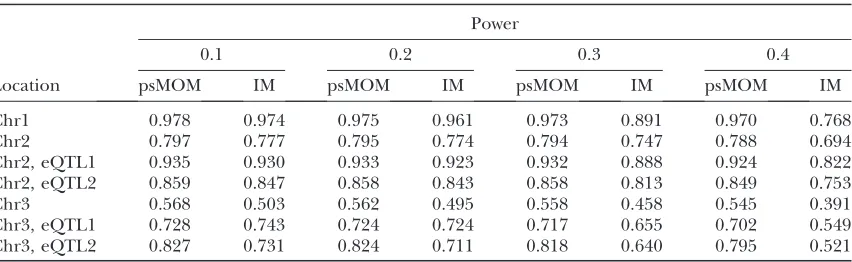
Simulation results:The results from a single simula-tion are shown in Figure 1 (results are representative of those observed in the other 19 simulations). The top graphs show results from psMOM and the bottom graphs show those from IM. The left graphs demonstrate the av-erage linkage evidence -posterior probabilities in psMOM and LOD posterior probabilities in IM; and the right graphs show transcript-specific HPD regions.
From the average linkage evidence shown in the left graphs, the two approaches considered are very similar: they each identify the regions for the single eQTL on chromosome 1 and the two unlinked eQTL on chro-mosome 3. Both MOM and marker regression miss the two linked eQTL, identifying a wide peak only in the middle region of chromosome 2. The interval-mapping approaches (psMOM and IM) further refined the eQTL underneath this wide peak.
Differences between the approaches are more pro-nounced when transcript-specific linkage evidence is
con-sidered. As shown in the right graphs of Figure 1, psMOM precisely identifies the eQTL correctly for most of the mapping transcripts. In contrast, the regions surround-ing the IM identifications are relatively wide. This result could be due to the way the LR normalization was done, to the fact that information shared across transcripts is not accounted for, or to both. To test the former, instead of HPD regions constructed from LOD posterior prob-abilities, we considered confidence intervals constructed using 1.5-LOD drop intervals around the peak LOD
score. As detailed in theImplementation of IMsection, this
procedure favors IM. Even so, the approach still pro-vided very imprecise estimates of eQTL location, much worse than those shown in Figure 1, and we do not re-commend this in practice.
The results for this single simulation hold across sim-ulations as shown in Tables 1–3. Table 1 reports power at varying thresholds averaged over 20 simulated data sets for each eQTL and each chromosome. For low thresh-olds, power is similar for both approaches, with psMOM showing slightly higher power. Table 2 shows that FDR from psMOM is well controlled for the three chromo-somes. The level stays the same under different thresh-olds. On the other hand, the FDR from IM is quite high at the 0.1 cutoff point; it decreases with increasing threshold, but with reduced power. Table 3 shows the specificity calculated over an average of 20 simulated
Figure 1.—Plots of average
data sets. The specificities are very similar for both ap-proaches and they are satisfactory.
Applications to data from a study of diabetes: The
data set considered here is discussed in detail in Lan
et al. (2006) and is available at GEO (Barrettet al. 2007), accession no. GSE3330. Briefly, 60 mice (29 males and
31 females) were selected from an F2 population
seg-regating for phenotypes associated with diabetes and
obesity (Stoehr et al. 2000). The population was
de-rived from B6 male and BTBR female parents. Selection was based on the selective phenotyping algorithm
devel-oped in Jinet al. (2004), which can substantially improve
sensitivity for QTL localization compared with random
sampling of the same sample size ( Jinet al. 2004). The
marker map consists of 145 microsatellite markers span-ning the 19 mouse autosomes, with an average inter-marker distance of 13 cM. Over 90% of the animals are genotyped at any given marker.
Liver total RNA was extracted from frozen tissue ples with RNAzol reagent (Tel-Test). Crude RNA sam-ples were purified with RNeasy mini columns (QIAGEN, Valencia, CA) before hybridization. The RNA samples were processed according to the Affymetrix Expression
Analysis technical manual. Expression levels for 45,265 probe sets (referred to hereinafter as transcripts) were measured using the MOE430A and MOE430B chips for
each of the 60 F2mice. Preprocessing and normalization
was done using robust multi-array average (RMA) (Irizarry
et al. 2003) to obtain a single normalized summary score of expression for each gene in each animal.
Both IM and psMOM were applied to the data; psMOM
accommodates F2populations by increasing the
num-ber of expression patterns. For example, with three ge-notype groups (0, 1, and 2) there are three latent means of interest and four non-null expression patterns for each
transcript t at each location lðm0
t;l 6¼m
1
t;l ¼m
2
t;l;m
0
t;l¼
m1
t;l6¼m
2
t;l;m
0
t;l ¼m
2
t;l6¼m
1
t;l;m
0
t;l6¼m
1
t;l 6¼m
2
t;lÞ.
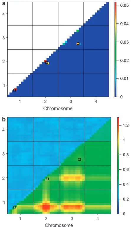
Posterior probabilities from psMOM and LOD pos-terior probabilities from IM were averaged across tran-scripts to identify the genomic regions of most interest. As in the simulation study, the average results from IM and from psMOM largely agreed (Figure 2a). However, when looking at a finer scale, one does observe impor-tant differences (Figure 2b). There are two locations in particular (on the distal regions of chromosomes 2 and 5) where psMOM shows some evidence for linkage but
TABLE 2
FDR averaged over 20 data sets
FDR
0.1 0.2 0.3 0.4
Location psMOM IM psMOM IM psMOM IM psMOM IM
Chr1 0.028 0.146 0.018 0.028 0.013 0.009 0.008 0.005 Chr2 0.024 0.152 0.016 0.025 0.009 0.009 0.007 0.002 Chr3 0.034 0.173 0.023 0.066 0.020 0.041 0.016 0.036
Standard errors were,0.01. Linkage thresholds were varied from 0.1 to 0.4. As noted in thePower and false discovery rate calculationsection, the FDR estimates shown heredo notconsider mapping transcripts that map outside the 10-cM window of the eQTL. Considering these transcripts greatly inflated the FDR for IM, alterna-tive methods for LOD profile normalization did not yield results better than those shown here.
TABLE 1
Power averaged over 20 data sets
Power
0.1 0.2 0.3 0.4
Location psMOM IM psMOM IM psMOM IM psMOM IM
Chr1 0.978 0.974 0.975 0.961 0.973 0.891 0.970 0.768 Chr2 0.797 0.777 0.795 0.774 0.794 0.747 0.788 0.694 Chr2, eQTL1 0.935 0.930 0.933 0.923 0.932 0.888 0.924 0.822 Chr2, eQTL2 0.859 0.847 0.858 0.843 0.858 0.813 0.849 0.753 Chr3 0.568 0.503 0.562 0.495 0.558 0.458 0.545 0.391 Chr3, eQTL1 0.728 0.743 0.724 0.724 0.717 0.655 0.702 0.549 Chr3, eQTL2 0.827 0.731 0.824 0.711 0.818 0.640 0.795 0.521
IM does not. To test whether the regions identified by psMOM might be meaningful, we consider the biolog-ical functions of identified transcripts.
We tested for functional enrichment among the
tran-scripts mapping to the two subpeaks (call thesetrans1a
andtrans1b) on the distal region of chromosome 2. Both sets show significant enrichment of lipid-metabolism
and fatty-acid-metabolism genes (P-values are 0.0016 and
0.0044, respectively). The lipid-metabolism group on the distal region of chromosome 2 coincides with the
lipid-metabolism cluster discovered in Lanet al. (2006).
Sev-eral QTL for obesity and related traits have been mapped
to this region (Stoehret al. 2000). As shown in Figure
2b, there is some evidence of linkage (a single peak) on the distal region of chromosome 2 provided by MOM (the first pass of psMOM at markers only). The tran-scripts mapping to this region did not show significant linkages for lipid metabolism or fatty acid metabolism
(P-values are 0.2465 and 0.2302, respectively) or for any
categories that appeared to be related to our diabetes or obesity phenotypes of interest.
In addition to the chromosome 2 linkages, we con-sidered two linkage peaks on the distal region of
chro-mosome 5, near the markerD5Mit240, as these peaks
are identified by psMOM alone. As on chromosome 2, tests here show enrichment for lipid-transport and fatty-acid-metabolism genes. In addition, the enrichment of genes responsible for positive regulation of metabolism
is highly significant (P-value¼0.002). A closer look at the
mapping list reveals some interesting members. They
include PPARaand PPARg, two major lipid-metabolism
transcription factors (Attieand Kendziorski2003).
Other interesting genes include fatty-acid-synthase genes (Fasn, Elovl6, Elovl5, and Fads2), lipid-transport genes (Scp2, Pltp, and Apoa4), and two fatty-acid-metabolism genes (Gpam and CD36). Taken together, these results provide some support for the peaks uniquely identified by psMOM.
DISCUSSION
We have extended the QTL mapping framework of
Sen and Churchill (2001) to accommodate
expres-sion phenotypes. The Bayesian formulation prescribed
by Senand Churchill(2001) and the
pseudomarker-sampling approach developed there is maintained. Our extension relies on specifying a more general form for the genetic model, the model relating phenotype to ge-notype. By fitting the full genetic model to all pheno-types simultaneously, information can be shared across transcripts through the estimated hyperparameters, which in many cases leads to improved inference.
The extended framework generalizes most eQTL map-ping approaches and in doing so facilitates their under-standing, evaluation, and precise comparison by revealing their specific characteristics in the context of a common notation, which in turn provides an improved environ-ment for addressing open questions and developing ideas for future methods. As an example, we considered a de-ficiency of the MOM model, namely that no information is provided between markers. Viewing MOM as a special case of the extended framework clarified how to address this deficiency using pseudomarkers. We expect that other open questions in the area of eQTL mapping can be more readily addressed in the context of this unified framework.
One such question might be the choice of an appro-priate threshold. In most eQTL studies to date, thresh-olds are varied and the one that yields a list with many transcripts while controlling some measure of false pos-itives at a reasonable level is used. A number of false positive measures have been considered; and, clearly, in-vestigators define ‘‘many’’ and ‘‘reasonable’’ quite
differ-ently in different contexts (Kendziorskiand Wang2006).
The framework presented here can be used to inves-tigate common approaches and perhaps to rigorously address this question.
Without exact knowledge of appropriate thresholds for either psMOM or IM, our evaluations were based on varying thresholds. There appears to be a slight advan-tage of psMOM over IM, likely due to the information shared across transcripts. For some thresholds, the ad-vantage is negligible; while for others, it is much more pronounced. A bigger advantage of psMOM is the pre-cision provided by the HPD regions. Analogous regions were constructed from the LOD profiles, but these pro-vided much less precise localization than the standard
HPD regions of psMOM. Indeed, as we noted inPower
TABLE 3
Specificity averaged over 20 data sets
Specificity
0.1 0.2 0.3 0.4
Location psMOM IM psMOM IM psMOM IM psMOM IM
Chr1 0.882 0.805 0.885 0.882 0.886 0.901 0.889 0.916 Chr2 0.884 0.806 0.887 0.883 0.889 0.905 0.891 0.922 Chr3 0.883 0.805 0.886 0.881 0.888 0.898 0.889 0.911
and false discovery rate calculationsection, the FDRs shown
in Table 2 did not consider differentially expressed
transcripts that mapped outside the 10-cM window of the eQTL. Considering these transcripts greatly inflated the FDR for IM. Considering alternative methods for LOD profile normalization did not yield results better than those shown here.
Finally, we have focused on representation of ap-proaches for single-eQTL mapping. The simulation re-sults show that the approaches can work well, even for two eQTL settings, much like single-QTL models can pro-vide information on multiple QTL. Of course,
single-QTL models will not work well when multiple single-QTL are tightly linked; and we here note that extensions of psMOM as presented are possible. In the context of the ex-tended framework, the extension is seen as changes in
fPk, where nowk.2. In particular, if a transcripttis
affected by two genotype locationsl1andl2, then four
latent means are of interest:m0t;;ð0l 1;l2Þ;m
1;0
t;ðl1;l2Þ;m 0;1
t;ðl1;l2Þ, and m1t;;ð1l
1;l2Þ. Here m
g1;g2
t;ðl1;l2Þ denotes the latent mean level of
expression for transcript t for the populations of
ani-mals with genotype (g1,g2) at locationsl1andl2. These
latent means can be arranged into 15 possible expression patterns, all of which may be of interest (see supplemental
Figure 2.—Average posterior probabilities
materials at http://www.genetics.org/supplemental/ for pattern specification and further detail). As before, of primary interest is the posterior probability of particular expression patterns. These can be calculated for any pat-tern of interest.
The approach was applied to the simulated data
de-scribed previously using all 15 expression patterns (i.e.,
k¼0, 1,. . ., 14). Results for one data set (representative
of the other 19) are presented in Figure 3. Figure 3a shows the posterior probabilities of P6 (additive model with equal effects) calculated for each marker pair averaged over all the transcripts. Because of symmetry, only the bottom triangle was plotted. The posterior probabilities from single-eQTL psMOM are shown on the diagonal.
The two eQTL on chromosomes 2 and 3 are located be-tween markers 5 and 7 and markers 3 and 9, respectively; psMOM identified them with fairly strong evidence.
Figure 3b shows the LOD scores derived from a stan-dard two-QTL IM approach. The top triangle contains LOD scores for epistatic interactions; the diagonal shows LOD scores from a single QTL model; the bottom trian-gle shows LOD scores for the additive model. Because the simulations did not include an interaction, the top triangle correctly shows very little linkage signal. In the bottom half, however, the entire path between markers 5 and 7 on chromosome 2 and markers 3 and 9 on chro-mosome 3 is highlighted with the highest LOD scores occurring at the marker pair regions between chromo-somes 1 and 2 and 2 and 3. In contrast, the graph from the two eQTL psMOM model gives improved localiza-tion of the true eQTL. This is promising evidence for the utility of extending psMOM to multiple eQTL.
One of the main obstacles in the multiple-eQTL model extension is the computational burden. The number of components in the mixture model grows rapidly with the number of loci under investigation. Fitting the full model can be a daunting task. A Dirichlet process mix-ture model for which the number of components is no
longer a bottleneck has been introduced (Chen2006)
and is currently under investigation.
The authors thank Gary Churchill, Jessica Flowers, Michael Newton, Saunak Sen, and Ping Wang for useful discussions. This work was sup-ported in part by National Institute of General Medical Sciences (R01GM076274-01) (G.M.) and National Institute of Diabetes and Digestive and Kidney Disease (R01DK066369-03) (C.K.).
LITERATURE CITED
Attie, A., and C. Kendziorski, 2003 Pcg-1alpha at the crossroads of
type 2 diabetes. Nat. Genet.34:244–245.
Barrett, T., D. Troup, S. Wilhite, P. Ledoux, D. Rudnevet al.,
2007 NCBI GEO: mining tens of millions of expression profiles– database and tools update. Nucleic Acids Res.33:D562–D566. Brem, R., G. Yvert, R. Clintonand L. Kruglyak, 2002 Genetic
dis-section of transcriptional regulation in budding yeast. Science
296:752–755.
Broman, K., H. Wu, S. Senand G. Churchill, 2003 R/qtl: Qtl
map-ping in experimental crosses. Bioinformatics19:889–890. Chen, M., 2006 Statistical methods for expression quantitative trait
loci (eQTL) mapping. Ph.D. Thesis, University of Wisconsin, Madison, WI.
Cox, N., 2004 An expression of interest. Nature430:733–734.
Cui, X., G. Hwang, J. Qiu, N. Bladesand G. Churchill, 2005
Im-proved statistical tests for differential gene expression by shrink-ing variance components estimates. Biostatistics6:59–75. Dupuis, J., and D. Siegmund, 1999 Statistical methods for mapping
quantitative trait loci from a dense set of markers. Genetics151:
373–386.
Gelfond, J., J. Ibrahimand F. Zou, 2006 Proximity model for
ex-pression quantitative trait loci (eqtl) detection. Biometrics62(1): 19–27.
Gentleman, R., 2004 Using GO for statistical analyses, pp. 171–180
inProceedings of COMPSTAT 2004 Symposium, Prague.
Irizarry, R., B. Hobbs, F. Collin, Y. Beazer-Barclay, K. Antonellis
et al., 2003 Exploration, normalization, and summaries of high
density oligonucleotide array probe level data. Biostatistics 4:
249–264.
Jansen, R., 1993 A general mixture model for mapping quantitative trait
loci by using molecular markers. Theor. Appl. Genet.85:252–260.
Figure 3.—Heat map from the two-dimensional model
Jansen, R., and P. Stam, 1994 High resolution of quantitative traits
into multiple loci via interval mapping. Genetics136:1447–1455. Jin, C., H. Lan, A. Attie, D. Bulutuglo, G. Churchill et al.,
2004 Selective phenotyping for increased efficiency in genetic mapping studies. Genetics168:2285–2293.
Kendziorski, C., M. Chen, M. Yuan, H. Lanand A. Attie, 2006
Sta-tistical methods for expression quantitative trait loci (eqtl) map-ping. Biometrics62:19–27.
Kendziorski, C., M. Newton, H. Lanand M. Gould, 2003 On
pa-rametric empirical bayes methods for comparing multiple groups using replicated gene expression profiles. Stat. Med.22:3899– 3914.
Kendziorski, C., and P. Wang, 2006 A review of statistical methods
for expression quantitative trait loci mapping. Mamm. Genome
17:509–517.
Lan, H., M. Chen, J. Byers, B. Yandell, D. Stapletonet al., 2006
Com-bined expression trait correlations and expression quantitative trait locus mapping. PLoS Genet.2: 0051–0061.
Lander, E., and D. Botstein, 1989 Mapping mendelian factors
un-derlying quantitative traits using rflp linkage maps. Genetics121:
185–199.
Mangin, B., B. Goffinetand A. Rebai, 1994 Constructing
confi-dence intervals for qtl location. Genetics138:1301–1308. Newton, M., C. Kendziorski, C. Richmond, F. Blattnerand K.
Tsui, 2001 On differential variability of expression ratios:
im-proving statistical inference about gene expression changes from microarray data. J. Comput. Biol.8:37–52.
Newton, M., A. Noueiry, D. Sarkarand P. Ahlquist, 2004
De-tecting differential gene expression with a semiparametric hier-archical mixture method. Biostatistics5:155–176.
Satagopan, J., B. Yandell, M. Newtonand T. Osborn, 1996 A
bayesian approach to detect quantitative trait loci using markov chain monte carlo. Genetics144:805–816.
Schadt, E., S. Monks, T. Drake, A. Lusis, N. Cheet al., 2003
Ge-netics of gene expression surveyed in maize, mouse and man. Nature422:297–302.
Sen, S., and G. Churchill, 2001 A statistical framework for
quan-titative trait mapping. Genetics159:371–387.
Smyth, G., 2004 Linear models and empirical bayes methods for
as-sessing differential expression in microarray experiments. Stat. Appl. Genet. Mol. Biol.3:1–27.
Stoehr, J., S. Nadler, K. Schueler, M. Rabaglia, B. Yandell
et al., 2000 Genetic obesity unmasks nonlinear interactions
be-tween murine type 2 diabetes susceptibility loci. Diabetes49:
1946–1954.
Tusher, V., R. Tibshiraniand G. Chu, 2001 Significance analysis of
microarrays applied to the ionizing radiation response. Proc. Natl. Acad. Sci USA98:5116–5121.
Visscher, P., R. Thompsonand C. S. Haley, 1996 Confidence
in-tervals in qtl mapping by bootstrapping. Genetics143: 1013– 1020.
Yi, N., 2004 A unified markov chain monte carlo framework for
map-ping multiple quantitative trait loci. Genetics167:967–975. Yi, N., and S. Xu, 2000 Bayesian mapping of quantitative trait loci
for complex binary traits. Genetics155:1391–1403.
Yvert, G., R. Brem, J. Whittle, J. Akey, E. Fosset al., 2003
Trans-acting regulatory variation insaccharomyces cerevisiaeand the role of transcription factors. Nat. Genet.35:57–64.
Zeng, Z., 1993 Theoretical basis of separation of multiple linked
gene effects on mapping quantitative trait loci. Proc. Natl. Acad. Sci USA90:10972–10976.
Zeng, Z.-B., 1994 Precision of mapping of quantitative trait loci.
Genetics136:1457–1468.
Communicating editor: R. W. Doerge
APPENDIX A
Assume transcripttis linked to locationl. For a backcross, there are then two distinct latent expression means, one
for each genotype group, denoted bym0
t;l andm
1
t;l. Consider a conditional distribution of measurements for animals
with genotype 0 given byy0
trjm
0
t fobsð jm0tÞ,r¼1,. . .,nand a prior distribution onm
0
t given bym
0
t jupu(m),t¼
1,. . .,T. The notation for dependence onlhas been suppressed. Under this model, the marginal distribution of
measurementsy0
t is given by
fP0ðyt0Þ ¼ð Y
n
r¼1
fobsðytrjm0tÞ !
pðm0
tÞdm0t: ðA1Þ
The same form holds fory1
t. The marginal distribution of measurementsytis then given byfP1(yt)¼fP0(yt0)fP0(y1t),
assuming conditional independence ofy0
t andy
1
t given the latent expression meansm
0
t andm
1
t.
For calculations presented here, we evaluate expression measurements on the log scale and assume a Gaussian
model forfobs(), with variances2;p() is also Gaussian with meanm0and variancet20. Hence, the hyperparameters
shared by all transcripts ares2,m
0, andt20. The joint predictive density,fP0, is then also Gaussian with meannvector (m0,
m0,. . .,m0) and exchangeable covariance matrix
Sn¼ ðs2ÞIn1ðt20ÞMn;
whereInis ann3nidentity matrix andMnis ann3nmatrix of ones. Further detail can be found in Kendziorski
et al. (2003).
APPENDIX B
The posterior distribution of the QTL location for transcripttis given by
pðgt ¼ljy;mÞ ¼ pðy;mj;gt ¼lÞpðgt ¼lÞ
In detail,
pðy;mjgt ¼lÞ
¼
Ð
pðyt;yt;m;gt ¼l;mÞdm pðgt ¼lÞ
¼
ð
pðyt;ytjm;gt¼l;mÞpðmÞpðmÞdm
¼
ð
pðytjm;gt ¼l;mltÞpðmltÞdmlt
ð
pðytjm;mtÞpðmtÞdmt
pðmÞ
¼pðytjm;gt¼lÞpðytjmÞpðmÞ;
whereytdenotes the matrix of expression phenotypes with transcripttomitted. We assume here (second equality)
that the distribution of the marker genotypes is independent of the eQTL location and latent expression means (this is
analogous to the assumption made in Senand Churchill(2001) in their Appendix A in justifying their final equality
with latent expression means here corresponding to their model parameters). We further assume that yt is
con-ditionally independent ofytgiven the latent expression mean for thetth transcript,mt, and that the latent expression
means are independent across transcripts (third equality). A similar derivation givesp(y,m)¼p(ytjm)p(ytjm)p(m).
Substituting these quantities into (B1), we have
pðgt ¼ljy;mÞ ¼pðytjm;gt¼lÞpðgt ¼lÞ
pðytjmÞ
: ðB2Þ
Note thatp(ytjm,gt¼l) in the numerator of (B2) can be further written as
pðytjm;gt ¼lÞ
¼pðyt;m;gt¼lÞ pðm;gt ¼lÞ
¼
Ð Ð
pðyt;m;gt ¼l;g;mltÞdg dmlt pðmÞpðgt¼lÞ
¼
ð ð
pðytjg;mltÞpðmltÞdmlt
pðgjm;gt ¼lÞdg
¼
ð
fP1lðytjgÞpðgjm;gt ¼lÞdg:
Here,grepresents the eQTL genotype of thetth transcript. We once again assume that the distribution of the marker
genotypes is independent of the eQTL location (second equality). The third equality follows from the assumption that
the expression levels of thetth transcript are independent of eQTL locations and marker genotypes given the eQTL
genotype and latent expression means (this is similar to the second equality of Sen and Churchill 2001, their
Appendix A, with latent expression means corresponding to their model parameters) and that the eQTL genotype is
independent of the latent expression means for transcripttgiven the eQTL locations and markers (similar to Senand
Churchill2001, their Appendix A, third equality). The last equality is given by the definition offP1. In summary, we have
pðgt ¼ljy;mÞ ¼K
ð
fP1lðytjgÞpðgjm;gt ¼lÞpðgt ¼lÞdg; ðB3Þ
forK ¼1=pðytjmÞ.
The notationpðml
tjgt ¼lÞimplies that integration with respect tomlt is a two-dimensional integral over the joint