A new non polynomial spline method for solution of linear and non linear third order dispersive equations

(1)

R E S E A R C H

Open Access

A new non-polynomial spline method for

solution of linear and non-linear third order

dispersive equations

Talat Sultana

1

_{, Arshad Khan}

2*

_{and Pooja Khandelwal}

3

*_{Correspondence:}

akhan1234in@rediﬀmail.com

2_{Department of Mathematics, Jamia}

Millia Islamia, New Delhi, India Full list of author information is available at the end of the article

Abstract

In this paper, a new three-level implicit method is developed to solve linear and non-linear third order dispersive partial differential equations. The presented method is obtained by using exponential quartic spline to approximate the spatial derivative of third order and finite difference discretization to approximate the first order spatial and temporal derivative. The developed method is tested on four examples and the results are compared with other methods from the literature, which shows the applicability and feasibility of the presented method. Furthermore, the truncation error and stability analysis of the presented method are investigated, and graphical comparison between analytical and approximate solution is also shown for each example.

MSC: 65D07; 65M12

Keywords: Spline function approximation; Third order dispersive equation; Stability analysis; Korteweg-de Vries (KdV) equation; Soliton

1 Introduction

In [4] Boussinesq and Korteweg-de Vries (KdV) equations described the problem of water waves and the long waves in which dispersive eﬀects are present. We use an exponential quartic spline function to develop a numerical method to approximate the solution of third order homogeneous and non-homogeneous linear dispersive equation in one space dimension withf(x,t) as a source term:

∂y(x,t)

∂t +μ

∂3y(x,t)

∂x3 =f(x,t), a≤x≤b,t> 0,μ> 0, (1.1)

with

y(x, 0) =g1(x), a≤x≤b, (1.2)

and

y(a,t) =γ0(t), t> 0,

yx(a,t) =γ1(t), t> 0,

yxx(a,t) =γ2(t), t> 0, ⎫ ⎪ ⎬ ⎪

⎭ (1.3)

(2)

whereγ0(t),γ1(t),γ2(t), andg1(x) are assumed to be continuous functions,tis time andx

is space variable [1,7].

In [1] theorems for the existence and uniqueness of solution of such dispersive equations are given. In [20,21], the criteria for deriving stability conditions of diﬀerence method were considered for the numerical solution of a third order linear dispersive equation. In [25], the analytical solution was obtained of such equations by using Adomian decomposition method, and in [19], such equations were solved numerically. The authors in [17] solved fourth order parabolic partial diﬀerential equation numerically by using parametric septic spline. Djidjeli and Twizell [7] developed numerical method for solution of third order linear dispersive equation with time-dependent boundary conditions.

We have also solved the third order non-linear dispersive equation named as Korteweg-de Vries (KdV) equation:

∂y(x,t)

∂t +εy(x,t)

∂y(x,t)

∂x +μ

∂3y(x,t)

∂x3 = 0, a≤x≤b,t> 0,μ> 0 (1.4)

with

y(x, 0) =g2(x), a≤x≤b, (1.5)

and

y(x,t) =γ3(t), x∈∂,t> 0,

yx(b,t) =γ4(t), t> 0,

(1.6)

where= [a,b]⊂R,εandμare positive parameters, andg2(x),γ3(t),γ4(t) are known

functions. This equation shows both dispersion and non-linearity [4,23,27].

The solution of Eq. (1.4) may exhibit solitons. Solitons are localized waves that propagate without change in their shape and velocity and are stable in mutual interaction just like the phenomenon of totally elastic collision in kinetics. The KdV type equations have been an important class of non-linear evolution equations with numerous applications in physical sciences and engineering ﬁelds see [5,8,12,18,23,24,26].

The existence and uniqueness of solutions of the KdV equation for appropriate condi-tions have shown in [11] . Many well-known numerical methods, such as finite difference scheme, finite element schemes, Fourier spectral methods and mesh-free radial basis func-tions (RBF), collocation method, multiquadric (MQ), multiquadric quasi-interpolation [3,

5,10,13–15,22,23,27,28], have been used to solve the KdV equation. Authors in [16] also used decomposition method for solution of KdV equation. The numerical solution was presented in [6] for the ﬁrst and ﬁfth order KdV equations. In [2], authors solved cou-pled Burgers’ equations using non-polynomial spline method. In [9], authors presented non-polynomial spline method for solving the generalized regularized long wave (GRLW) equations.

(3)

Here, we obtain a derivation of exponential quartic spline and its relations in Sect.2. In Sect.3, we present the formulation of our methods along with boundary equations for both the linear and non-linear dispersive equations. In Sect.4, a class of methods and truncation error are given. Stability analysis is discussed in Sect.5. Numerical evidences and comparison with other available methods are included in Sect.6to show the accuracy of our method. The presented method is tested on four examples. Finally, conclusion is presented in Sect.7.

2 Exponential quartic spline

Let a set of grid points in the interval [a,b] be such that

xj=a+jh, j= 0(1)n,h=

b–a

n . (2.1)

We also denote the function valuey(xj) byyj.

LetEj(x,t) be the exponential quartic spline at the grid point (xj,t) given by

Ej(x,t) =a1j(t)eτ(x–xj)+a2j(t)e–τ(x–xj)+a3j(t)(x–xj)2+a4j(t)(x–xj) +a5j(t) (2.2)

for eachj= 0, 1, . . . ,n, wherea1j,a2j,a3j,a4j,a5jare unknown coeﬃcients andτ is a free parameter. We determine the unknown coeﬃcients in (2.2) from the interpolatory condi-tionsEj(xj,t) =yj(t),Ej(xj+1,t) =yj+1(t),Ej(xj,t) =mj(t),Ej(3)(xj,t) =Tj(t), andE(3)j (xj+1,t) =

Tj+1(t) as given below:

a1j(t) = 1

τ3

(Tj+1–Tje–θ) (eθ_–_e–θ₎ ,

a2j(t) = 1

τ3

(Tj+1–Tjeθ) (eθ_–_e–θ₎ ,

a3j(t) = 1

h2(yj+1–yj) –

1

hMj–

1

h2a1j(t)

eθ–θ– 1–a2j(t)

h2

e–θ+θ– 1, (2.3)

a4j(t) =mj–a1j(t)τ+a2j(t)τ,

a5j(t) =yj–a1j(t) –a2j(t).

Applying the continuity conditions of ﬁrst and second derivatives ofEj(x,t) at the knots, that is,E_j(xj) =Ej–1(xj),Ej(xj) =Ej–1(xj), and using (2.3) yields the following relations:

mj+mj–1=h2(α1Tj+α1Tj–1) +

2

h(yj–yj–1), (2.4)

mj–mj–1=h2(β1Tj+1+β2Tj+β3Tj–1) +

1

(4)

where

α1=

θ(eθ_–_e–θ_{) – 2(}_eθ₊_e–θ_{) + 4}

θ3₍_eθ_–_e–θ₎ ,

β1=

θ2_{– (}_eθ₊_e–θ_{) + 2}

θ3₍_eθ_–_e–θ₎ ,

β2=

θ(eθ_–_e–θ_{) –}_θ2₍_eθ₊_e–θ₎

θ3₍_eθ_–_e–θ₎ ,

β3=

θ2_–_θ₍_eθ_–_e–θ_{) + (}_eθ₊_e–θ_{) – 2}

θ3₍_eθ_–_e–θ₎ .

(2.6)

Using Eqs. (2.4) and (2.5), we obtain the following method:

h3(pTj+1+qTj+qTj–1+pTj–2) = –yj+1+ 3yj– 3yj–1+yj–2, j= 2(1)(n– 1), (2.7)

where the coeﬃcients p=β1 andq= –α1+β1+β2. Asτ →0 that is θ →0, we have

(p,q)−→(–₂₄1, –11₂₄). Now, the operatorxfor any functionW is supposed to have the following form according to Eq. (2.7):

xWj=pWj+1+qWj+qWj–1+pWj–2. (2.8)

3 Derivation of the method

Let the regionR= [a≤x≤b]×[t> 0] be discretized by a set of pointsRh,kwhich are the vertices of grid points (xj,tm), wherexj=jh,j= 0(1)n,nh=b–a, andtm=mk,m= 0, 1, 2, 3, . . . . The quantitieshin space andkin time directions are mesh sizes.

3.1 Spline solution for linear dispersive equation

In this section we develop an approximation for (1.1) in which the time and space deriva-tives are replaced by a ﬁnite diﬀerence and exponential quartic spline respectively. Equa-tion (1.1) is discretized as:

k–1

2 δt

1 +σ δ2_t–1ym

j +μTjm=fjm, (3.1)

whereTm j =E

(3)

(xj,tm) is the third order spline derivative at (xj,tm) w.r.t. the space variable,

fm

j =f(xj,tm),yjmis the approximate solution of (1.1) at (xj,tm),δtis the central difference operator w.r.t.tandσis a parameter such that finite difference approximation to the time derivative is ofO(k) for arbitraryσ.

Operatingxon both sides of (3.1) and after some simpliﬁcations, we obtain the fol-lowing method:

δt

pym_j₊₁+qym_j +qy_jm_–1+pym_j_–2+2kμ

h3

1 +σ δ_t2–ym_j₊₁+ 3ym_j – 3ym_j_–1+ym_j_–2

(5)

The ﬁnal method (3.2) may be written in the schematic form as follows: one more equation atj= 1, i.e., at the end of the range of integration in order to have a closed form solution foryj. We discretize the boundary conditions in (1.3) and develop the following boundary equation of accuracyO(k+h2_):

–21ym₀ + 24ym₁ – 3ym₂ – 18hym₀– 6h2ym₀= 0, j= 1, (3.4) 3.2 Spline solution for non-linear dispersive equation

In the similar manner, Eq.(1.4) is discretized as follows:

k–1

Operatingxon both sides of (3.5) and after some simpliﬁcations, we obtain the fol-lowing method:

The schematic form of method (3.6) is given by

(6)

= order to have a closed form solution foryj. We discretize the boundary conditions in (1.6) and develop the following boundary equation of accuracyO(k+h2_):

–ym

4 Truncation error and a class of methods

Expanding (3.2) or (3.6) in a Taylor series in terms ofy(xj,tm) and its derivatives and using (1.1) or (1.4) respectively, we obtain the truncation error as follows:

TEm_j = 2(p+q)kDt– (p+q)khDtDx+

Here, the following class of methods are obtained:

Case 1: Ifp+q= 0, then various methods ofO(k+h)for arbitrary values ofσ are ob-tained.

(7)

5 Stability analysis and convergence

Theorem Methods(3.3)and(3.7)are conditionally stable forσ ≥(1₂ –₂1_r),where r> 0,

p+q= 0,andφ=θ 2.

Proof Here the stability analysis of any one of methods (3.3) or (3.7) will be investigated, and it can be investigated for other method in the same manner. For this, we use the Von Neumann method. Let the solution of (3.3) at the point (xj,tm) is

ym_j =ξmejiθ_, _(5.1)

wherei=√–1,θis real andξin general is complex.

We get the following equation after putting (5.1) in the homogeneous part of (3.3):

Uξ2+Vξ+W= 0, (5.2)

where

U=Peiθ₊_Q₊_Re–iθ₊_Se–2iθ_,

V=Neiθ+ 3 – 3e–iθ+e–2iθ,

W= –Seiθ+R+Qe–iθ+Pe–2iθ.

The necessary and suﬃcient condition for method (3.3) to be stable is|ξ| ≤1. For this, we obtain the following condition:

4Nsin3φ/(p+q)2– 410pq+ 9p2+q2+ 12σ2r2sin2φ

+ 164p2+ 2(3p–q)σr+ 8σ2r2sin4φ

– 32pq–p2– (3p–q)σr– 2σ2r2sin6φ1/2≤1.

Simplifying and puttingp+q= 0, we deduce that method (3.3) is conditionally stable for

σ≥(1₂–₂1_r), wherer> 0 andφ=θ₂.

The present method is convergent by Lax theorem as the stability criterion is satisﬁed.

6 Numerical simulation and comparison

In this section, the presented three-level implicit method based on exponential quartic spline is tested on four examples. The following norms are used in this paper:

L∞=_1≤max

i≤n

yana(i) –yapp(i),

L2=

n

i=1

yana(i) –yapp(i) 2

,

RMS=

_n

i=1

yana(i) –yapp(i)

2

n,

(8)

whereyanais analytical andyappis approximate solution of third order dispersive equation

for our method.

Example1 (Linear homogeneous case) Consider the following linear homogeneous dis-persive equation [7]

∂y

∂t +μ

∂3y

∂x3 = 0, 0≤x≤1,t≥0,μ> 0

with

y(x, 0) =cosx, 0≤x≤1

and

y(0,t) =cosμt, ∂y

∂x(0,t) = –sinμt,

∂2y

∂x2(0,t) = –cosμt, t≥0.

The analytical solution is

y(x,t) =cos(x+μt).

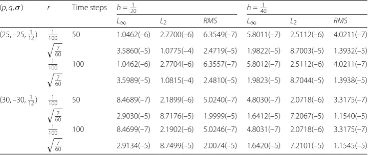
The computational results of this example for μ= 1 are tabulated in Tables 1 and2. Table 1 shows L∞, L2 and RMS errors for h= ₂₀1, ₄₀1; r= ₁₀₀1 ,

7 60; σ =

1

12 and time

steps = 50, 100 for diﬀerent values of parameterspandq. The comparison ofL∞ error

between our method and in [7] withp= 30, 75;r= 1; h= 0.1;σ =₁₂1; time steps = 100 forx= 0.1, 0.2, . . . , 0.9 is tabulated in Table2. Also the comparison between analytical and approximate solution forh=₃₂1,r=√1

6, and time steps = 100 is shown graphically in Fig.1.

Example 2 (Linear non-homogeneous case) Consider the following linear

non-homo-geneous dispersive equation [25]

∂y

∂t +μ

∂3_y

∂x3 = –π

3_cos₍_π_x₎_cos_t_–_sin₍_π_x₎_sin_t_, ₀_≤_x_≤_1,_t_≥_0,_μ_{> 0}

Table 1 L_∞,L2andRMSerrors for Example1

(p,q,σ) r Time steps h= 1

20 h=

1 40

L∞ L2 RMS L∞ L2 RMS

(25, –25,₁₂1) ₁₀₀1 50 1.0462(–6) 2.7700(–6) 6.3549(–7) 5.8011(–7) 2.5112(–6) 4.0211(–7)

7

60 3.5860(–5) 1.0775(–4) 2.4719(–5) 1.9822(–5) 8.7003(–5) 1.3932(–5) 1

100 100 1.0462(–6) 2.7704(–6) 6.3557(–7) 5.8012(–7) 2.5112(–6) 4.0211(–7)

7

60 3.5989(–5) 1.0815(–4) 2.4810(–5) 1.9823(–5) 8.7044(–5) 1.3938(–5)

(30, –30,₁₂1) ₁₀₀1 50 8.4689(–7) 2.1899(–6) 5.0240(–7) 4.8030(–7) 2.0718(–6) 3.3175(–7)

7

60 2.9030(–5) 8.7176(–5) 1.9999(–5) 1.6412(–5) 7.2067(–5) 1.1540(–5) 1

100 100 8.4699(–7) 2.1902(–6) 5.0246(–7) 4.8031(–7) 2.0718(–6) 3.3175(–7)

7

(9)

Table 2 Comparison ofL_∞error with [7] for Example1

Time steps r h x (p,q,σ) (30, –30,₁₂1)

(p,q,σ) (75, –75,₁₂1)

[7]

100 1 0.1 0.1 2.14(–6) 7.22(–5) 1.70(–3)

0.2 4.99(–5) 2.49(–5) 5.00(–4)

0.3 4.50(–5) 2.88(–5) 4.00(–4)

0.4 8.42(–5) 4.20(–5) 7.00(–4)

0.5 6.71(–5) 4.00(–5) 8.00(–4)

0.6 9.30(–5) 4.63(–5) 9.00(–4)

0.7 5.91(–5) 3.62(–5) 1.00(–3)

0.8 6.73(–5) 3.35(–5) 1.10(–3)

0.9 1.28(–5) 1.35(–5) 1.10(–3)

Figure 1Comparison between analytical and approximate solution

with

y(x, 0) =sin(πx), 0≤x≤1

and

y(0,t) = 0, ∂y

∂x(0,t) =πcost,

∂2y

∂x2(0,t) = 0, t≥0.

y(x,t) =sin(πx)cost.

The computational results of this example forμ= 1 are tabulated in Tables3and4. The

L∞,L2andRMSerrors are tabulated in Table3for the same values of parameters as taken

(10)

Table 3 L_∞,L2andRMSerrors for Example2

(p,q,σ) r Time steps h=₂₀1 h=₄₀1

L_∞ L2 RMS L_∞ L2 RMS

(25, –25,₁₂1) ₁₀₀1 50 6.4058(–6) 1.4539(–5) 3.3356(–6) 5.2848(–6) 2.0991(–5) 3.3613(–6)

7

60 1.4202(–4) 3.5828(–4) 8.2196(–5) 1.8686(–4) 7.2452(–4) 1.1601(–4) 1

100 100 6.4058(–6) 1.4539(–5) 3.3356(–6) 5.2848(–6) 2.0991(–5) 3.3613(–6)

7

60 1.4202(–4) 3.5828(–4) 8.2196(–5) 1.8686(–4) 7.2452(–4) 1.1601(–4)

(30, –30,₁₂1) ₁₀₀1 50 9.3013(–6) 2.1326(–5) 4.8926(–7) 3.9930(–6) 1.5921(–5) 2.5494(–6)

7

60 2.4187(–4) 6.1364(–4) 1.4078(–4) 1.4128(–4) 5.4912(–4) 8.7930(–5) 1

100 100 9.3013(–6) 2.1326(–5) 4.8926(–7) 3.9930(–6) 1.5921(–5) 2.5494(–6)

7

60 2.4187(–4) 6.1364(–4) 1.4078(–4) 1.4128(–4) 5.4912(–4) 8.7930(–5)

Table 4 L_∞error for Example2

Time steps r h x (p,q,σ)

(25, –25, 1 12)

(p,q,σ) (50, –50, 1

12)

100 1 0.05 0.1 2.19(–4) 6.94(–4)

0.3 2.72(–4) 8.63(–4)

0.5 1.28(–6) 1.58(–6)

0.7 2.74(–4) 8.66(–4)

0.9 2.20(–4) 6.96(–4)

0.1 0.1 1.20(–3) 1.37(–3)

0.3 2.81(–3) 3.29(–3)

0.5 6.59(–3) 7.21(–3)

0.7 1.60(–2) 1.77(–2)

0.9 1.43(–2) 1.57(–2)

1

12; time steps = 100 forx= 0.1, 0.3, 0.5, 0.7, 0.9. Figure2shows the graphical comparison

between analytical and approximate solution forh=₆₄1,r=₁₀₀1 and time steps = 100.

Example3 (Non-linear single soliton case) Consider a propagation of single solitary wave of non-linear KdV Eq. (1.4) withε= 6,μ= 1 [5,15,23,27] and

y(x, 0) =κ 2sech

2

√

κ

2 x–L

, a≤x≤b.

y(x,t) = κ 2sech

2

√

κ

2 (x–κt) –L

.

The functionsγ3(t) andγ4(t) are extracted from the analytical solution. The

computa-tional results are tabulated in Tables5–7. TheL∞,L2andRMSerrors withL= 7;κ= 0.5;

[a,b] = [0, 40];p= 25;k= 0.001, 0.0001;n= 40, 80, 120, 160, 200;σ=₁₂1 andt= 1, and the comparison ofL∞ error with [15,23,27] with changes p= 30;k= 0.01, 0.001;n= 200;

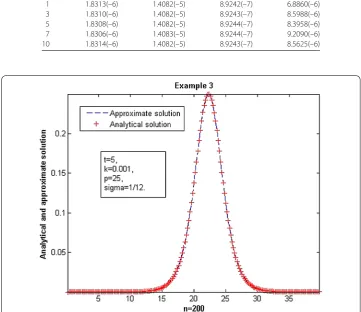
t= 1, 2, . . . , 5 are tabulated in Table5 and Table 6, respectively. Table7 shows L∞, L2

andRMSerrors and comparison with [5] withL= 10;κ= 0.14; [a,b] = [30, 80];p= 100;

(11)

Table 5 L_∞,L2andRMSerrors forp= 25,σ=₁₂1,t= 1,κ= 0.5,L= 7, [a,b] = [0, 40] for Example3

n k= 0.001 k= 0.0001

40 6.1192(–5) 1.1111(–4) 1.7793(–5) 6.7755(–6) 1.3143(–5) 2.1045(–6) 80 7.3626(–5) 1.7866(–4) 2.0101(–5) 7.3800(–6) 1.7870(–5) 2.0106(–6) 120 6.5572(–5) 1.9993(–4) 1.8327(–5) 6.5602(–6) 1.9994(–5) 1.8328(–6) 160 5.1806(–5) 2.1081(–4) 1.6718(–5) 5.1798(–6) 2.1082(–5) 1.6719(–6) 200 4.8556(–5) 2.5697(–4) 1.8216(–5) 4.8559(–6) 2.5697(–5) 1.8216(–6)

Table 6 Comparison ofL_∞error with [5,15,23,27] forp= 30,σ=₁₂1,κ= 0.5,L= 7,n= 200, [a,b] = [0, 40] for Example3

t Our method IMQQI [23] Our method [5] MQQI [27] MQ [15] IMQ [15]

k= 0.01 k= 0.001

1 4.2123(–4) 1.6728(–4) 4.2120(–5) 1.8048(–5) 1.5259(–3) 1.7923(–5) 6.9584(–5) 2 4.2238(–4) 2.3758(–4) 4.2235(–5) 3.0373(–5) 2.8677(–3) 3.0151(–5) 1.9553(–4) 3 4.2123(–4) 2.3758(–4) 4.2120(–5) 4.0088(–5) 4.1428(–3) 3.9839(–5) 3.8286(–3) 4 4.2237(–4) 3.1348(–4) 4.2234(–5) 4.8347(–5) 5.3859(–3) 4.7835(–5) 5.9098(–3) 5 4.2126(–4) 3.4136(–4) 4.2122(–5) 5.6090(–5) 6.8141(–3) 5.4599(–5) 8.3667(–3)

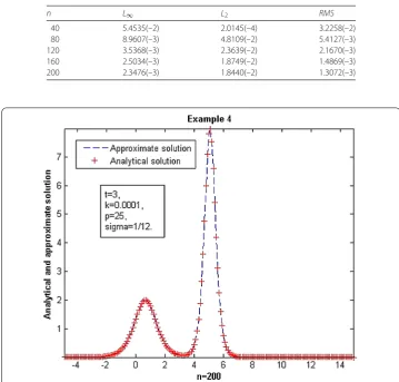
Example4 (Non-linear soliton interaction case) Consider a propagation of two solitary waves of non-linear KdV Eq. (1.4) withε= 6,μ= 1 [5,15,23,27] and

y(x, 0) = 12 3 + 4cosh(2x) +cosh(4x) {3cosh(x) +cosh(3x)}2

, –5≤x≤15.

y(x,t) = 12 3 + 4cosh(2x– 8t) +cosh(4x– 64t) {3cosh(x– 28t) +cosh(3x– 36t)}2

(12)

Table 7 L_∞,L2andRMSerrors forp= 100,σ=₁₂1,k= 0.001,κ= 0.14,L= 10,n= 250, [a,b] = [30, 80]

and comparison ofL_∞error with [5] for Example3

t Our method [5]

L∞ L2 RMS L∞

1 1.8313(–6) 1.4082(–5) 8.9242(–7) 6.8860(–6)

3 1.8310(–6) 1.4082(–5) 8.9243(–7) 8.5988(–6)

5 1.8308(–6) 1.4082(–5) 8.9244(–7) 8.3958(–6)

7 1.8306(–6) 1.4083(–5) 8.9244(–7) 9.2090(–6)

10 1.8314(–6) 1.4082(–5) 8.9243(–7) 8.5625(–6)

Table 8 Errors forp= 10,σ=₁₂1,k= 0.00001,h= 0.1 and comparison ofL_∞error with [5,15,27] for

Example4

t Our method [5] MQQI [27] MQ [15] IMQ [15]

L_∞ L2 RMS L_∞

0.01 3.9805(–4) 1.6355(–3) 1.1594(–4) – 7.7405(–3) 9.2114(–4) 2.2071(–2) 0.05 1.7221(–3) 4.4270(–3) 3.1382(–4) – 6.3762(–2) 2.9608(–2) 7.2316(–2) 0.1 2.8226(–3) 6.8615(–3) 4.8640(–4) 5.6353(–3) 1.6196(–1) 1.2806(–2) 1.0121(–1)

0.2 3.5029(–3) 8.2930(–3) 5.8787(–4) 2.3376(–2) – – –

0.3 3.5726(–3) 8.4542(–3) 5.9930(–4) 5.9437(–2) – – –

Similarly, the functionsγ3(t) andγ4(t) are extracted from the analytical solution. The

com-putational results are tabulated in Tables8–10. Table8and Table9show the comparison ofL∞,L2 andRMSerrors with [5,15,23,27] withp= 10;k= 0.0001, 0.00001;n= 200;

σ=₁₂1 andt= 0.01, 0.05, 0.10, 0.15, 0.20, 0.3. Also, theL∞,L2andRMSerrors withp= 100;

k= 0.0001;n= 40, 80, 120, 160, 200;σ= 1

12 andt= 1 are tabulated in Table10. Figure4

shows the graphical comparison between analytical and approximate solution forn= 200,

(13)

Table 9 Comparison ofL_∞,L2andRMSerrors with [23] forp= 10,σ=₁₂1,k= 0.0001,n= 200 for

Example4

t Our method [23]

0.01 4.0120(–3) 1.6335(–4) 1.1579(–3) 4.0579(–3) 9.9105(–3) 6.9903(–4) 0.05 1.7249(–2) 4.4265(–2) 3.1378(–3) 4.1003(–2) 1.0295(–1) 7.2619(–3) 0.10 6.5572(–2) 6.8612(–2) 4.8638(–3) 9.1691(–2) 2.3373(–1) 1.6486(–2) 0.15 5.1806(–2) 7.9154(–2) 5.6111(–3) 1.3257(–1) 3.4201(–1) 2.4124(–2) 0.20 4.8556(–2) 8.2929(–2) 5.8786(–3) 1.6644(–1) 4.3607(–1) 3.0758(–2)

Table 10 L_∞,L2andRMSerrors forp= 100,σ=121,k= 0.0001,t= 1 for Example4

n L∞ L2 RMS

40 5.4535(–2) 2.0145(–4) 3.2258(–2)

80 8.9607(–3) 4.8109(–2) 5.4127(–3)

120 3.5368(–3) 2.3639(–2) 2.1670(–3)

160 2.5034(–3) 1.8749(–2) 1.4869(–3)

200 2.3476(–3) 1.8440(–2) 1.3072(–3)

7 Conclusion

(14)

Funding

Jamia Millia Islamia, New Delhi, India.

Competing interests

The authors declare that they have no competing interests.

Authors’ contributions

All authors drafted the manuscript, and they read and approved the ﬁnal version.

Author details

1_{Department of Mathematics, Lakshmibai College, University of Delhi, New Delhi, India.}2_{Department of Mathematics,}

Jamia Millia Islamia, New Delhi, India.3_{Department of Mathematics, M. L. V. Textile and Engineering College, Bhilwara,} India.

Publisher’s Note

Springer Nature remains neutral with regard to jurisdictional claims in published maps and institutional aﬃliations.

Received: 16 May 2018 Accepted: 15 August 2018

References

1. Agarwal, R.P.: Boundary Value Problems for Higher Ordinary Diﬀerential Equations. World Scientiﬁc, Singapore (1986) 2. Ali, K.K., Raslan, K.R., El-Danaf, T.S.: Non-polynomial spline method for solving coupled Burgers’ equations. Comput.

Methods Diﬀer. Equ.3(3), 218–230 (2015)

3. Carey, G.F., Shen, Y.: Approximation of the KdV equation by least squares ﬁnite element. Comput. Methods Appl. Mech. Eng.93, 1–11 (1991)

4. Craig, W., Goodman, J.: Linear dispersive equations of airy types. J. Diﬀer. Equ.87, 38–61 (1990)

5. Dehgan, M., Shokri, A.: A numerical method for KdV equation using collation and radial basis functions. Nonlinear Dyn.50, 111–120 (2007)

6. Djidjeli, K., Price, W.G., Twizell, E.H., Wang, Y.: Numerical methods for the solution of the third and ﬁfth order dispersive Korteweg-de Vries equation. J. Comput. Appl. Math.58, 307–336 (1995)

7. Djidjeli, K., Twizell, E.H.: Global extrapolations of numerical methods for solving a third order dispersive partial diﬀerential equation. Int. J. Comput. Math.41, 81–89 (1999)

8. Dodd, R.K., Eilbeck, J.C., Gibbon, J.D., Morris, H.C.: Solitons and Nonlinear Wave Equations. Academic Press, New York (1982)

9. El-Danaf, T.S., Raslan, K.R., Ali, K.K.: Non-polynomial spline method for solving the generalized regularized long wave equation. Commun. Math. Model. Appl.2(2), 1–17 (2017)

10. Feng, B.F., Mitsui, T.: A ﬁnite diﬀerence method for the Korteweg-de Vries and the Kadomtsev–Petiashvili equation. J. Comput. Appl. Math.90, 95–116 (1998)

11. Gardner, C.S., Grrne, M.J., Kruskal, M.D.: Method for solving Korteweg-de Vries equation. Phys. Rev. Lett.19, 1095–1097 (1967)

12. Gardner, C.S., Marikawa, G.K.: The eﬀect of temperature of the width of a small amplitude solitary wave in a collision free plasma. Commun. Pure Appl. Math.18, 35–49 (1965)

13. Geyikli, T., Kaya, D.: An application for modiﬁed KdV equation by the decomposition method and ﬁnite element method. Appl. Math. Comput.69(2), 971–981 (2005)

14. Helal, A.M., Mehanna, M.S.: A comparison between two diﬀerent methods for solving KdV–Burgers equation. Chaos Solitons Fractals28(2), 320–326 (2006)

15. Islam, S., Khattak, A.J., Tirmizi, I.A.: A meshfree method for numerical solution of KdV equation. Eng. Anal. Bound. Elem.

32, 849–855 (2008)

16. Kaya, D.: On the solution of a Korteweg-de Vries like equation by the decomposition method. Int. J. Comput. Math.

72, 531–539 (1999)

17. Khan, A., Sultana, T.: Numerical solution of fourth order parabolic partial diﬀerential equation using parametric septic spline. Hacet. J. Math. Stat.45(4), 1067–1082 (2016)

18. Korteweg-de Vries, D.J., de Vries, G.: On the change in form of long waves advancing in rectangular canal and on a new type of long stationary waves. Philos. Mag.39, 422–443 (1895)

19. Mechee, M., Ismail, F., Hussain, Z.M., Siri, Z.: Direct numerical methods for solving a class of third order partial diﬀerential equations. Appl. Math. Comput.247, 663–674 (2014)

20. Mengzhao, Q.: Diﬀerence scheme for the dispersive equation. Computing31, 261–267 (1983)

21. Miller, J.H.: On the location of zeros of certain classes of polynomials with application to numerical analysis. J. Inst. Math. Appl.8, 397–406 (1971)

22. Refik, B.A.: Exponential finite-difference method applied to Korteweg-de Vries for small times. Appl. Math. Comput.

160, 675–682 (2005)

23. Sarboland, M., Aminataei, A.: On the numerical solution of nonlinear Korteweg-de Vries equation. Syst. Sci. Control Eng.3, 69–80 (2015)

24. Washimi, H., Taniuti, T.: Propagation of ion acoustic solitary waves of small amplitude. Phys. Rev. Lett.17, 996–998 (1966)

25. Wazwaz, A.M.: An analytic study on the third order dispersive partial diﬀerential equations. Appl. Math. Comput.142, 511–520 (2003)

26. Wijngaarden, L.V.: On the equation of motion for mixtures of liquid and gas bubbles. J. Fluid Mech.33, 465–474 (1968)

27. Xiao, M.L., Wang, R.H., Zhu, C.H.: Applying multiquadric quasi-interpolation to solve KdV equation. J. Math. Res. Exposition31, 191–201 (2011)