DOI: 10.1534/genetics.104.029686
The Genetic Architecture of Response to Long-Term Artificial Selection
for Oil Concentration in the Maize Kernel
Cathy C. Laurie,*
,1Scott D. Chasalow,* John R. LeDeaux,* Robert McCarroll,* David Bush,*
Brian Hauge,* Chaoqiang Lai,* Darryl Clark,
†Torbert R. Rocheford
†and John W. Dudley
†*Monsanto Company, St. Louis, Missouri 63167 and†Department of Crop Sciences, University of Illinois, Urbana, Illinois 61801 Manuscript received April 6, 2004
Accepted for publication August 16, 2004
ABSTRACT
In one of the longest-running experiments in biology, researchers at the University of Illinois have selected for altered composition of the maize kernel since 1896. Here we use an association study to infer the genetic basis of dramatic changes that occurred in response to selection for changes in oil concentration. The study population was produced by a cross between the high- and low-selection lines at generation 70, followed by 10 generations of random mating and the derivation of 500 lines by selfing. These lines were genotyped for 488 genetic markers and the oil concentration was evaluated in replicated field trials. Three methods of analysis were tested in simulations for ability to detect quantitative trait loci (QTL). The most effective method was model selection in multiple regression. This method detectedⵑ50 QTL accounting forⵑ50% of the genetic variance, suggesting that⬎50 QTL are involved. The QTL effect esti-mates are small and largely additive. About 20% of the QTL have negative effects (i.e., not predicted by the parental difference), which is consistent with hitchhiking and small population size during selection. The large number of QTL detected accounts for the smooth and sustained response to selection throughout the twentieth century.
T
HE genetic architecture of a quantitative trait con- tries. An objective of our study is to identify genes that sists of a set of parameters that explain the genetic may be used to increase the oil concentration of maize component of trait variation within or among popula- kernels through plant breeding or genetic engineering.tions. These parameters include the number of quanti- The experiment reported here originated in 1896
tative trait loci (QTL) affecting the trait, their locations when C. G. Hopkins began the Illinois long-term selec-in the genome, the frequencies of alternative genotypes tion lines, which have become a “textbook” example of segregating at the QTL, the pattern of linkage disequi- the power of artificial selection (see review byDudley
libria among QTL, and the magnitudes of additive, andLambert2004). From an open-pollinated variety
dominance, and epistatic effects. Knowledge of genetic of maize, Hopkins started two populations that were architecture has applications in two areas: (1) the identi- selected divergently for the percentage of kernel dry fication of genes with utility in agriculture and/or treat- weight that consists of oil (“oil concentration” or “per-ment of disease and (2) making inferences about the centage of oil”). These populations are called Illinois evolutionary processes that maintain genetic variation high oil (IHO) and Illinois low oil (ILO). In each gener-and those that cause divergence between populations.
ation and each population, bulked kernels from each Here we report a study of oil variation in maize that has
of a number of ears (half-sib families) were analyzed both types of application.
and the highest (or lowest) 20% of ears were selected to The kernels of a modern maize (Zea maysL.) hybrid
be parents of the next generation. This selection was typically containⵑ4% oil, 9% protein, 73% starch, and
carried on throughout the twentieth century at the Uni-14% other constituents (mostly fiber). The caloric
con-versity of Illinois and continues to this day for IHO with tent of oil is 2.25 times greater than that of starch on
no sign of a plateau in response. At generation 89, se-a weight bse-asis se-and livestock feeding studies hse-ave shown
lection in ILO was discontinued because of poor viability a greater rate of weight gain per pound of feed for
high-and an oil concentration so low that it cannot be measured oil (⬎7%) than for normal maize (reviewed byLambert
accurately. At this point, the populations had changed 1994 and Lambert et al. 2004). Therefore, high-oil
from 4.7% oil to 19.3% in IHO and 1.1% in ILO. maize is in demand as a source of animal feed, which
Currently, the oil concentration of IHO is ⵑ20%, is the primary use of maize grown in developed
coun-which is far greater than levels in commercial germ-plasm. Unfortunately, the yield and other agronomic characteristics of IHO are poor (Dudley et al. 1974;
1Corresponding author:14031 Shadow Oaks Way, Saratoga, CA 95070.
E-mail: [email protected] Lambert1994), so the population itself is not used in
commercial production. However, the genes that confer chromosomal regions that may be useful for increasing oil concentration in commercial maize germplasm. high oil in IHO may have utility in two ways. First, it
might be possible to separate the beneficial effects on oil from the negative effects on agronomic
characteris-MATERIALS AND METHODS
tics by focused introgression of oil alleles into
high-yielding germplasm through plant breeding. Second, Notation:r2
LDis a measure of linkage disequilibrium,R2TMis the coefficient of multiple determination for regression of
identification of the genes that actually cause oil
varia-trait value on the genotype scores of multiple markers, and
tion may provide good candidates for genetic
engi-R2
MMis the coefficient of multiple determination of the
regres-neering of high-yielding germplasm through plant
sion of the genotype score of one marker on the genotype
transformation. If variation in the sequence of a gene scores of multiple other markers.
causes variation in oil, it suggests that the system of Germplasm and field trials:The association study
popula-tion originated from a cross between IHO and ILO performed
oil production and storage in maize is sensitive to the
at generation 70 of selection when the oil concentrations were
structure and/or amount of the corresponding gene
estimated for IHO as 16.7% and for ILO as 0.4% (Dudley product. Therefore, even if the natural alleles of these
andLambert2004). Approximately five to seven individuals
genes have small effects, it is possible that artificial of each parental population were crossed to produce a hybrid changes in expression or amino acid sequence can pro- population, which was randomly mated for 10 generations.
During random mating,ⵑ200 plants per generation were used
duce larger effects of utility in agriculture.
(100 as male and 100 as female). One RM10:S1 line was
de-Here we report on QTL identification and
character-rived from each of 500 different RM10 plants in the following
ization in a population derived from the Illinois
long-way. Each RM10 plant was selfed to produce an ear of S1
ker-term selection lines. At generation 70 of selection, several nels (S1 ear). The kernels from one S1 ear were planted to-individuals each of IHO and ILO (both polymorphic gether in a single row and the plants were selfed to produce
ears containing S2 kernels (S2 ears). One S2 ear was selected
populations) were crossed to produce a hybrid
popula-at random to represent an RM10 plant. The kernels on this
tion, which was randomly mated for 10 generations
S2 ear (and their progeny) constitute an RM10:S1-derived line.
(RM10). The RM10 individuals were selfed to produce
Kernels from each of the S2 ears were divided into two parts:
500 RM10:S1 lines that constitute the study population. 50 kernels to be used for DNA extraction and the remaining These lines were genotyped for a set of 488 genetic kernels (ⵑ50) for additional crosses to produce material for
phenotypic analysis. For each line, the S2 kernels for
pheno-markers and oil was evaluated in replicated field trials
typic analysis were planted adjacent to a stiff stalk tester
(Mon-in the partially (Mon-inbred l(Mon-ines and (Mon-in hybrids produced
santo 7051) and two sets of crosses were made. The tester was
by crossing each line to an inbred tester. This design
fertilized with pollen from the S2 plants to produce hybrid
provides considerable power and resolution for QTL offspring and the S2 plants were intermated within each S1 detection and localization because the sample size is family to produce inbred offspring. The inbred and hybrid
kernels from each of 500 lines were planted in replicated field
relatively large, the trait was evaluated with replication
trials.
on a line basis (i.e., family mean rather than individual
The field layout was an ␣(0, 1) incomplete block design
measurements), and the 10 generations of random
mat-(PattersonandWilliams1976) with two replicates per
loca-ing provide multiple opportunities for recombination. tion. Each replicate consisted of one row each of 500 lines Standard methods of linkage analysis for quantitative arranged in 50 blocks of 10 lines each. The ␣(0, 1) design
specifies that each line occurs together in a block with any
traits, such as QTL interval mapping, are not directly
other line either 0 or 1 times. To produce kernels for
composi-applicable to this population because parental phases
tional analysis,ⵑ10 sib-matings were made within each row,
of the S1 individuals are unknown. However, this
popu-with one pollen parent per mating and each plant used as
lation is quite suitable for linkage disequilibrium (LD) pollen parent only once. This procedure yielded six to eight mapping and we have analyzed the experiment as an ears per line per replicate, from which kernels were bulked
for compositional analysis. Three locations were used in each
association study (LanderandSchork 1994). In this
of 2 years, for a total of 12 replicates each for inbred and
case, a single admixture event between IHO and ILO
hybrid seed. The locations were Urbana, Illinois; Monmouth,
created LD between genes with different allelic
frequen-Illinois; and Williamsburg, Iowa.
cies. The subsequent 10 generations of random mating Phenotypic trait measurements:Kernel composition was es-eliminated essentially all associations between unlinked timated by near-infrared spectroscopy (DyerandFeng1997).
For hybrids, whole-kernel samples were analyzed at Monsanto
markers and most of those between loosely linked
mark-by near-infrared transmittance with an Infratec Grain Analyzer
ers, yet retained associations between closely linked
instrument. For the inbred samples, kernels were dried to a
marker/QTL pairs.
relatively uniform moisture level, ground, and then analyzed
The study presented here has the following major ob- at the University of Illinois by near-infrared reflectance using jectives: (1) select a statistical method appropriate for a Dickey-John instrument (Hymowitzet al.1974;Dudleyand Lambert1992). Both methods provide estimates of the
per-multiple-QTL identification in an association study and
centage of kernel dry weight that consists of oil.
evaluate its performance in simulations; (2) describe
If there were no missing samples, the total number of
repli-the genetic architecture of oil variation in sufficient
cates for each line would be 12. The mean (SD) replicate
num-detail to provide insight into the population genetic bers are 11.9 (0.3) for hybrid and 11.0 (1.3) for inbred lines. processes involved in sustained response to long-term Markers and genotyping:For each RM10:S1 line, 50 S2
ker-nels were germinated and grown in the greenhouse. Then all
50 seedlings were lyophilized and bulked together for DNA level of association with A that is not missing inX(say locus B). Then the observed two-locus genotypic frequencies for extraction. The genotypes of individual S1 plants were inferred
from this bulk DNA sample. In addition, DNA was extracted loci A and B were used to estimate the frequencies of the three A locus genotypes conditional on the B locus genotype from individual plants of IHO and ILO of generation 70
(par-ents of the hybrid population). DNA was extracted by a stan- of individualX. The most frequent A locus genotype (condi-tional on B) was designated as the missing genotype. The dard procedure (Dellaportaet al.1983).
DNA samples were genotyped for a set of biallelic single- complete genotypic data matrix with 97.7% observed and 2.3% imputed calls is referred to as genotypic matrix C.
nucleotide polymorphism (SNP) markers using the 5⬘nuclease
Taqman assay described byLivak(2003). For quality control, Analysis of variance of phenotypic data: The model for analysis of variance of the phenotypic observations is standards of known genotype (six each of the three types)
and six negative controls were included in every set of 192
Yijkl⫽ ⫹ ␣i⫹ j⫹(␣)ij⫹ ␥k{j}⫹ ␦l{kj}⫹εijkl, (1) samples analyzed. Such standards were used to estimate the
accuracy of genotype calls in production runs at 0.996 (n⫽ where ␣i is the effect of theith line,jis effect of the jth
137,115). combination of location and year (locyr), (␣)
ijis the line⫻ The markers assayed in this experiment are from a set of
locyr interaction,␥k{j}is the effect of thekth replicate (rep) SNPs discovered in the parents of three mapping populations
nested within locyr,␦l{kj}is effect of thelth block nested within that are unrelated to the Illinois germplasm. The genetic map
locyr⫻rep, andεijklis the residual. All effects are considered distances provided are from a Monsanto reference map, which
to be random. Hybrid and inbred observations were analyzed is based on a composite of information from these three
popu-separately. ANOVA of theⵑ6000 observations for each trait lations.
(500 lines⫻3 locations⫻2 replicates) was done using PROC The primer and probe sequences for the Taqman
geno-MIXED in SAS with the REML option (SASInstitute1999). typing assays are available on request of J. R. LeDeaux at
Mon-This analysis provides variance component estimates and best santo. Access requires agreement that the sequences will be
linear unbiased predictors (BLUPs) of the line effects. Likeli-used only for noncommercial research and will not be trans- hood-ratio statistics were calculated to test the significance of ferred to a third party. the line⫻locyr interaction and the main effect of lines, as
To maximize the chances of detecting marker-trait associa- described by
Littellet al.(2002, p. 103). tions, markers run on the association study population were A broad-sense heritability
H2was estimated as the fraction selected to have a large allelic frequency difference between of the variation among line means within an experiment that the parental populations, IHO and ILO. These frequencies is due to genetic effects,
were estimated from 25 individuals each of IHO and ILO and markers were selected that have a frequency difference of at
H2⫽ ˆ
2
␣
ˆ2
␣⫹(1/b)ˆ2
␣⫹(1/bc)ˆ2 ε
, (2)
least 0.60 or, if one parental population was fixed, a difference of at least 0.40. This selection resulted in 472 markers (ⵑ30%
of those tested), to which 16 markers with smaller frequency whereˆ2is a variance component estimate,b⫽6 location⫻ differences were added to fill some gaps in the genetic map. year combinations, andc⫽2 replicates within each location⫻ This brings the total to 488 markers (in 470 different genes), year combination.
of which 440 are nonredundant in the sense that all pairs The relationship between phenotype and genotype was ana-haver2
LD⬍0.99, wherer2LDis defined below. The mean (SD) lyzed using the predicted line means (BLUP plus intercept of the allelic frequency differences for the 440 nonredundant from the random-model ANOVA).
markers is 0.76 (0.22). The expected heterozygosity in the Marker-trait associations:Initially, one-way ANOVAs were RM10:S1 population is high at most loci: the 0th, 25th, 50th, done to analyze the effect of each marker separately. The 500 75th, and 100th percentiles of the distribution of 2p(1⫺p), predicted line means of one type (hybrid or inbred) were wherepis the allelic frequency, are 0.04, 0.37, 0.45, 0.49, and analyzed with the phenotypic value as dependent variable and 0.50, respectively. the marker genotype (coded as a categorical variable with three Linkage disequilibrium estimation:A maximum-likelihood levels) as independent variable. The significance of an additive procedure was used to estimate linkage disequilibrium (LD) effect was tested as a contrast between the two homozygous in the RM10:S1 from unphased diploid genotypes. Solutions classes and that of a dominance effect as a contrast between to this problem for randomly mating populations have been the heterozygous class and the mean of the two homozygous well studied (WeirandCockerham1979;ExcoffierandSlat- classes. These single-marker ANOVA models were fit in S-PLUS
kin1995; Fallinand Schork2000). We modified this ap- with the “lm” function (S-PLUS 2000, 1999). Epistatic interac-proach to estimate LD for individuals obtained by selfing from tions between pairs of markers were tested in two-way ANOVA a randomly mated population. For details, see Section A and using PROC GLM of SAS.
The ANOVA indicated that dominance and epistatic inter-Figure S1 of supplemental materials (http://www.genetics.org/
supplemental/). Results are presented for a measure of LD, action effects are very small compared with additive effects (seeresults). Therefore, subsequent analyses of marker-trait
r2
LD, defined as follows. Consider two loci, locus A with alleles
Aanda, and locus B with allelesBandb. The allelic frequen- associations were done using regression analyses of strictly additive models (using PROC REG of SAS software). Three cies arePx(wherexrepresentsA, a,B, orb), the frequency
of the haplotypeABisPAB, andD⫽PAB⫺PAPB. Thenr2LD⫽ types of regression analyses, described in detail below, were done: (1) single-marker regression, (2) stepwise multiple
re-D2/(P APaPBPb).
Imputation of missing genotypes:In the association study, gression with MAXR/BIC, and (3) covariate regression. For stepwise regression, we used the option “MAXR” of 500 lines were genotyped for 488 SNP markers. One line had
an excessive number of missing genotypes and was dropped PROC REG in SAS, which is described in the following quota-tion (where “R2” isR2
TM). “The MAXR method begins by find-from the analysis. Among the remaining 499 lines, 2.3% of
scores were missing. The mean (SD) of the number of scores ing the one-variable model producing the highestR2. Then another variable, the one that yields the greatest increase in for each line is 477 (16).
Missing genotypes were imputed by using information from R2, is added. Once the two-variable model is obtained, each of the variables in the model is compared to each variable associated markers. To impute a missing genotype at locus A
determines if removing one variable and replacing it with Each simulated data set was analyzed by single-marker re-gression, MAXR/BIC, and covariate regression. In each case, the other variable increasesR2. After comparing all possible
switches, the MAXR method makes the switch that produces the analyses includedmmarkers that are assigned to be true QTL (m⫽40, 50, or 60) and 440⫺mmarkers that are not the largest increase inR2. Comparisons begin again, and the
process continues until the MAXR method finds that no switch QTL (but may be in linkage disequilibrium with QTL). For each simulated data set and each method of analysis, the best could increaseR2. Thus, the two-variable model achieved is
considered the ‘best’ two-variable model the technique can set ofkmarkers was selected. In the case of single-marker and covariate regressions, the best set consists of thek markers find. Another variable is then added to the model, and the
comparing-and-switching process is repeated to find the ‘best’ with lowestP-value (in thet-test that the regression coefficient equals zero). In the case of MAXR, the best set consists of the three-variable model, and so forth” (SASInstitute1999, p.
2948). MAXR was used to identify the best model of a given kmarkers that maximize R2
TM according to the MAXR algo-rithm. A total of 16 values of kwere used in the analysis of dimension (number of markers) for the range of 1–120
markers. each simulated data set. These values were set by 15 different
P-value thresholds and the BIC stopping rule. TheP-value The best model dimension was selected by minimizing a
criterion that is equivalent to a maximum likelihood with a pen- thresholds are 0.00001 (the Bonferroni criterion with ␣ ⫽ 0.05), 0.00005, 0.0001, 0.0005, 0.001, 0.003, 0.006, 0.01, 0.015, alty on model complexity. In general, the criterion is⫺2log
lik⫹py, where log lik is the maximized log-likelihood,p is 0.02, 0.025, 0.03, 0.04, 0.05, and 0.10. The number of markers having aP-value from single-marker regression less than or the number of parameters in the model (the number of
mark-ers plus one for the intercept), andyis a penalty factor. Here equal to the threshold determined the value ofk. Thus, for each simulated data set, 48 sets of markers were selected (3 we used the Bayesian information criterion (BIC; Schwarz
1978;Rawlingset al.1998): BIC⫽nln(SSR)⫹pln(n)⫺n methods⫻16 values ofk).
In the simulations, all 440 markers analyzed were classified ln(n), wherenis the sample size andSSRis the residual sum
of squares. In this casey⫽ln(n)⫽ln(499)⫽6.2. into one of five categories: (a) the marker is a true QTL, it was selected, and the estimated regression coefficient has the The covariate regression analysis provides a test focused on
each marker (say marker x) by regressing phenotypic value same sign as the effect of that QTL in the model; (b) the marker is a true QTL and it was selected, but the coefficient on marker x and a set of covariate markers. The covariate
markers were selected to account for variation in the trait, has the wrong sign; (c) the marker is a true QTL and was not selected; (d) the marker is a non-QTL and was selected; or but have small correlation with markerx, as follows. Start with
a potential set of covariates consisting of the set of markers (e) the marker is a non-QTL and was not selected. LetNxbe the number of markers in categoryx.
selected by the MAXR/BIC procedure. Do multiple regression
of the genotypic score of markerx on the genotypic scores The quality of selected markers was assessed in four ways: of the set of potential covariates. If the coefficient of multiple
1. The fraction of QTL selected was calculated asNa/(Na⫹ determination of this regression (R2
MM) is⬎0.10, remove the
Nb⫹Nc). marker that contributes the most toR2
MMand perform the
re-2. The fraction of markers selected that are considered as gression again. The process continues untilR2
MM⬍0.10. The
non-QTL was calculated as (Nb⫹Nd)/(Na⫹Nb⫹Nd). The covariate regression procedure is similar in concept to
com-contribution ofNbto this quantity is generally very small posite interval mapping (JansenandStam1994;Zeng1994).
unless the total number selected is very large. For example, Simulations:All simulated data sets are based on genotypic
the average ofNb/(Nb⫹Nd) is⬍0.6% for all three methods data matrix C (i.e., on the actual, not simulated, genotypes).
of regression when the number of markers selected is speci-The phenotypic value of theith individual (i⫽1, . . . , 499)
fied by BIC. was simulated as
3. The distance between each selected marker and the nearest QTL on the genetic map was calculated. This distance is
Yi⫽ ⫹
兺
mj⫽1
jXij⫹εi, (3)
zero when the marker is a QTL.
4. The degree of association between each selected marker where is the mean,mis the number of QTL,jis the ef- and the set of QTL was estimated as theR2
MMof the regres-fect of thejth QTL (partial regression coefficient),Xijis the sion of the genotypic score of that marker on the genotypic genotypic score at thejth QTL (⫺1, 0, or 1) and theεiare scores of the QTL. The value ofR2
MMis one when the marker independent and identically distributed N(0, 2). For each
is a QTL. model, 100 replicate data sets were simulated and analyzed.
The simulation models of phenotypic value are based on three key results of applying MAXR/BIC selection to the
ob-RESULTS served data set for the inbred lines: (1) 50 markers selected,
(2) a set of 50 partial regression coefficients, and (3) a residual
Linkage disequilibrium:Several different measures of
variance of 0.43. We refer to this set of results as model A. In
two-locus LD have been described (DevlinandRisch all simulation models, the residual variance (2) equals 0.43.
Four different types of models were simulated (sets B, C, D, 1995;Weir1996). In the context of detecting
marker-and E)—see Table 1. In all cases, a set ofnmarkers (n⫽40, trait associations, we prefer ther2
LDmeasure because of 50, or 60) was chosen at random from the total set of 440 to its relationship to the additive genetic variance. In a be QTL. In models of type E, no further constraints were
randomly mating population, the additive genetic
vari-imposed. In types B, C, and D, random marker sets were
re-ance associated with a neutral marker equals the
prod-jected unless they met certain constraints regarding
associa-tions between QTL and/or the magnitude of the variance of uct ofr2
LD(between marker and QTL) and the additive phenotypic values. In models of type B, only 50 QTL were genetic variance due to the QTL. This relationship fol-simulated and the effects of those QTL were selected at ran- lows algebraically from equations for the additive ge-dom without replacement from the set of 50 coefficients from
netic variance provided by Nielsenand Weir(1999).
model A. For all other models, the effects were assigned to
The RM10:S1 population studied here was derived by
QTL by random sampling with replacement from the
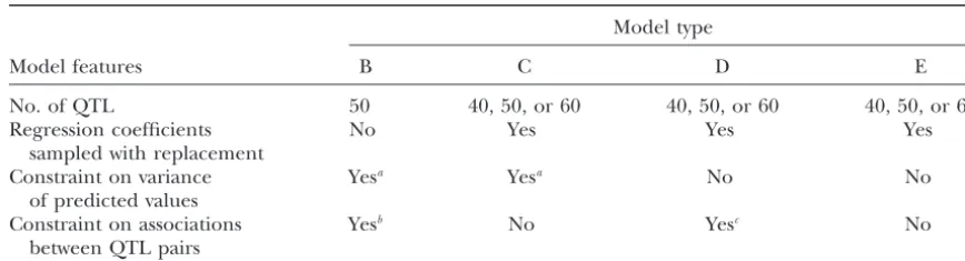
popu-TABLE 1
Summary of simulation models
Model type
Model features B C D E
No. of QTL 50 40, 50, or 60 40, 50, or 60 40, 50, or 60
Regression coefficients No Yes Yes Yes
sampled with replacement
Constraint on variance Yesa Yesa No No
of predicted values
Constraint on associations Yesb No Yesc No
between QTL pairs
Seematerials and methodsfor similarities among the models and further explanation of differences. aThe variance of predicted phenotypic values was constrained to be within 5% of the variance for model A (0.75).
bThe intrachromosomal distribution of LD between QTL pairs was constrained to match that of model A within bins of 0.1 (which has the effect of reducing the level of LD between QTL compared with randomly selected sets).
cNo pair of QTL was allowed to haver2
LDⱖ0.25.
lation. Although the relationship between additive ge- main effect of lines is extremely significant (P⬍10⫺16).
netic variance of a marker and that of an associated QTL The line⫻locyr (genotype-by-environment) interaction does not hold exactly for this population, numerical is also highly significant in both cases (P⫽4.7⫻10⫺5
calculations show that it is approximately correct (data for hybrids andP⫽ 2.0⫻10⫺14for inbreds).
not shown). If we assume that the pattern ofr2
LDvalues Variance component and broad-sense heritability
esti-between markers is similar to that esti-between markers and mates (Table 2) have three notable features: QTL, the former may serve as an indication of our ability
1. Despite being highly significant, the magnitude of to detect QTL through marker associations.
the variance component for the genotype-by-environ-Ther2
LDwas estimated for all pairs of the 488 markers
ment interaction is less than one-tenth that of the run on the association study population. For the 110,529
line component. pairs of unlinked markers (i.e., on different
chromo-2. The variance components for hybrids are much somes or⬎50 cM apart), the 0th, 25th, 50th, 75th, and
smaller than those for inbreds, but the heritability is 100th percentiles of the distribution ofr2
LDare 0, 0.0002,
about the same. Evidently, the phenotype of hybrids 0.001, 0.003, and 0.05. So, there is very little, if any, LD
between unlinked markers, as expected for a population that has undergone 10 generations of random mating. Therefore, any observed marker-trait association is al-most certainly due to linkage between the marker and a QTL.
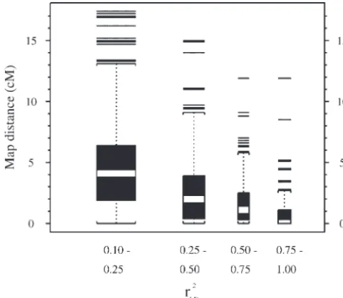
Figures 1 and 2 show the relationship between r2 LD
and genetic map distance between pairs of linked mark-ers (ⱕ50 cM apart). LD declines with map distance, as expected, and is very small for markers⬎20 cM apart (maximum is 0.07). The median map distance between loci with very highr2
LD values (0.75–1.00) is 0 cM and
75% of all suchr2
LDvalues occur between loci within 1.1
cM of each other. Among all pairs of linked markers, only 7.1% haver2
LD ⱖ 0.25 and the median and third
quartile of map distance for this group are 1 and 2.6 cM, respectively. Thus, if anr2
LD ⬎ 0.25 were required
to detect a significant marker-trait association, most of those associations would indicate a marker-QTL dis-tance of less than a few centimorgans.
Phenotypic data analysis:Analyses of variance of the Figure 1.—Relationship between linkage disequilibrium raw observations of percentage of oil were performed (r2
LD) and genetic map distance between 8299 linked marker pairs (⬍50 cM apart).
from 4.4 to 10.5% for inbreds and from 4.1 to 6.0% for hybrids. The corresponding ranges for most commer-cial inbreds and hybrids are from 3.4 to 5.4% and from 3.6 to 4.8%, respectively. This comparison indicates the potential of genes segregating in the study population to increase oil beyond the current norm of commercial germplasm.
Dominance and epistasis:The ordinary test for domi-nance is to contrast phenotypic values of the heterozy-gote with the mean of the two homozyheterozy-gotes. Such a test can be performed with the data from the RM10:S1 lines, but the interpretation is different from usual because the phenotypic data for each line are obtained from a pool of family members that will be a mixture of geno-types in families derived from a heterozygous parent. Therefore, the effect of any dominance that may exist is diluted. There is no true dominance in the hybrids because they are produced by crossing each line to a common inbred tester. Consequently, the heterozygous Figure2.—Distribution of genetic map distance for linked
lines produce hybrids that are an equal mixture of the
marker pairs (⬍50 cM apart) that occur in four bins with
genotypes produced by the two types of homozygous
respect to theirr2
LDvalues. In this “box plot” format, the solid
box extends from the first to the third quartiles (and thus lines.
contains 50% of the observations). The box is divided at the A total of 440 t-tests for dominance, one for each median by an open bar. A vertical line extends from the box to marker, were performed with each set of phenotypic the greatest (and smallest) observation within 1.5 interquartile
data (using the predicted line means). WithP ⬍0.05,
ranges. All observations outside these limits are plotted
indi-26 tests were significant in the hybrids and 25 in the
vidually. The width of each box is proportional to sample size, which is 499, 281, 141, and 166 from left to right. Ther2
LDbin inbreds, with an overlap of 10 markers significant in from 0.0 to 0.10 (not shown) has 7212 pairs for which the both. The expected number of significant tests is 22 first quartile equals 11.9 cM, the median equals 23.8 cM, and (5% of 440) if all tests are independent. Because of the third quartile equals 36.5 cM.
LD among markers, the tests are not all independent. Nevertheless, it appears that there is little or no evidence for dominance.
is more stable, but the total variance among line
Two-way analyses of variance were used to detect inter-means is less, as expected since all hybrids have one
actions between pairs of markers. All pairs of 440 mark-of their parents in common.
ers were tested in both inbreds and hybrids. In a total 3. The high heritability estimates (96% in both cases)
of 193,160 tests, 5.7% were significant at the 5% level, are very favorable for detecting marker-trait
associa-1.2% at the 1% level, and 0.15% at the 0.1% level. tions.
These numbers are similar when the tests are limited to markers with significant additive effects on the trait. The predicted line means of percentage of oil range
TABLE 2
Variance components and summary statistics for percentage of oil in the kernel
Inbreds Hybrids
Variance components Estimate 95% C.I.a Estimate 95% C.I.a
Locyr 1.05 0.40–6.92 0.029 0.011–0.191
Rep(locyr) 0.07 0.03–0.40 0.002 0.001–0.013
Block(locyr⫻rep) 0.20 0.18–0.24 0.010 0.009–0.013
Line 1.22 1.07–1.40 0.105 0.092–0.120
Locyr⫻line 0.10 0.08–0.13 0.004 0.003–0.008
Residual 0.47 0.44–0.50 0.049 0.047–0.052
Summary statistics
Variance of BLUPs 1.16 0.10
Heritability 0.96 0.96
Mean 7.06 4.92
Because many of the pairwise tests are not independent, the expectation that a fraction␣of tests are significant with P- value ⬍ ␣ does not necessarily apply precisely. Nevertheless, these results show very little evidence for two-locus epistatic interactions.
The results described so far suggest little genotype-by-environment interaction, dominance, or epistasis. Therefore, subsequent analyses of marker-trait associa-tions were done using regression analysis of the pre-dicted line means with strictly additive models and marker genotypes coded as 1 forAA, 0 forAa, and⫺1 foraa(whereAis the allele with the higher frequency in IHO).
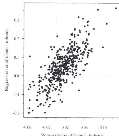
Single-marker regressions:A single-marker regression analysis was performed for each of 440 markers in both the hybrid and inbred data. A regression coefficient was estimated and the null hypothesis that the coefficient equals zero was evaluated with a standardt-test. Estab-lishing a threshold for declaring significance of thet-test requires a consideration of the multiple testing issue. Here we use the “false discovery rate” (FDR) approach described byStorey(2002) andStoreyand
Tibshir-ani(2003). The FDR is the expected proportion of null Figure3.—Relationship between inbreds and hybrids with hypotheses declared false (i.e., “significant”) that are respect to the coefficient (slope) estimated by single-marker
regression. Each point represents 1 of 440 markers.
not false. We use a threshold for significance that corre-sponds to an FDR of 5%, which means that we expect
ⵑ5% of the markers declared significant to be false
MAXR stepwise regression:Model selection for multi-leads (i.e., not associated with QTL).
ple regression proceeded according to the following For the inbreds, 66 of 440 markers (15%) have an
steps: FDRⱕ0.05 (andPⱕ0.014). For the hybrids, 54 of 440
markers (12%) have an FDRⱕ 0.05 (andP ⱕ0.010). a. A class of models was selected first—namely, linear models with only additive effects because of the weak Thirty markers were significant in both inbreds and
evidence for nonadditive effects. hybrids. The observation of a relatively large proportion
b. The search for a set of models within this class was of markers having significant association to the trait is
accomplished by the MAXR algorithm. Ideally, one not surprising, given that all markers were selected to
would like to examine all possible combinations of show a large frequency difference between the parental
a given number of regressors, but this is not feasible populations, which are very divergent in trait value.
for the large number of potential regressors in this The additive effect for the trait associated with each
experiment. The MAXR method is a compromise marker is estimated by the regression coefficient. The
between the exhaustive search and the more limited magnitude of this effect is expected to be greater in
search provided by standard forward, backward, or inbreds than in hybrids because the contrast between
stepwise methods (Hocking1976). homozygous lines in inbreds isAA vs. aa, whereas the
c. Models of the same dimension (number of re-corresponding contrast in hybrids isAA vs. Aa(for an
gressors) were compared and the one with maximum AA tester) or Aa vs. aa (for an aa tester). Figure 3
R2
TMwas selected as the best model of a given
dimen-shows that this is the case. Figure 3 also dimen-shows that the
sion. correlation between effects in inbreds and hybrids is
d. Models with different dimensions were compared high (r⫽ 0.75,P⬍0.0001). Similarly, the correlation
according to the value of the BIC and the model between predicted line means in inbreds and hybrids
with the minimum BIC value was selected as the best is also high (r⫽0.73,P⬍0.0001). Consistency in effect
model over all. between inbreds and hybrids is expected in the absence
of dominance and epistasis. For the inbreds, 50 markers were selected with
Significant markers occur on all 10 chromosomes and r2
TM⫽ 62%. Among the 50 coefficients, 38 are positive
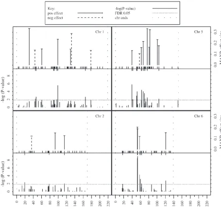
Figure4.—Summary of single-marker regression and MAXR/BIC analysis of inbred line data. Each quadrant contains a pair of plots of data for one chromosome (“Chr”). The top plot shows the MAXR/BIC analysis and the bottom plot shows the single-marker regressions. The MAXR/BIC plots give the estimated effect size for each single-marker selected (i.e., the magnitude of the partial regression coefficient). Some of the coefficients are positive (“pos effect”) and others are negative (“neg effect”). The single-marker regression plots give⫺log(P- value) for all markers (where theP- value is for thet- test that the coefficient equals 0). The dotted lines labeled “chr ends” represent the first and last markers on the Monsanto composite genetic map. The short vertical lines at the bottom of the MAXR-effect size plots are the positions of all markers analyzed. The short vertical lines at the top of the⫺log(P- value) plots are the positions of markers with aP- value that is less than the FDR 0.05 threshhold.
selected, which account for 43% of the trait variance. The markers selected by MAXR/BIC tend to be unas-sociated, since the procedure selects only markers that Among the 39 coefficients, 33 are positive and 6 are
negative. A total of 16 markers were selected in both increase the r2
TM in combination with other markers.
The level of association can be estimated by ther2 MMof
inbreds and hybrids and, in each of those cases, the
sign of the coefficient is the same. The distributions of regression of the genotype score of each selected marker on the others. The median value ofr2
MMis 0.16 for the
the 50 inbred and 39 hybrid coefficients are shown in
Figure 5. As expected, the range of values for hybrids 50-marker inbred model and 0.11 for the 39-marker hybrid model. The selected markers are also well distrib-(⫺0.09 to 0.08) is considerably smaller than the range
for inbreds (⫺0.34 to 0.34). These ranges are similar to uted on the genetic map. For the inbred data, the 50 selected markers are distributed across all 10 chromo-those for the coefficients from single-marker regression
important regressors and including extraneous ones (BromanandSpeed2002). No statistical theory applies directly to solving this problem, but simulations can be used to evaluate the performance of model selection procedures. Of course, the usefulness of simulation re-sults depends on the relevance of the simulation model to the biological situation at hand. Therefore, the mod-els simulated here have several features of the observed data set. The observed genotypic data were used in all of the simulations so that the complex pattern of linkage disequilibria would be preserved. To simulate the phe-notypic values, we assumed that the model derived by MAXR/BIC analysis of the observed data represents a rough approximation to the real biological situation. We then simulated variations of this model, analyzed the data by the MAXR/BIC and other methods, and compared results of the analysis to the model simulated. Four related questions are addressed:
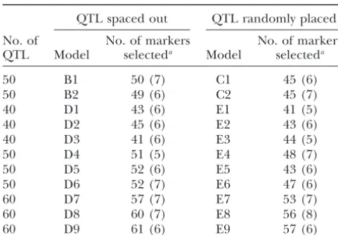
1. Can the MAXR/BIC procedure be used to estimate the number of different QTL? This question can be addressed by asking whether the BIC stopping rule designates a number of markers similar to the actual Figure5.—Distribution of effect size estimates for markers number of QTL in the simulated model. Table 3 selected by MAXR/BIC. The fraction of markers having a shows the results for 11 models in which 40, 50, or MAXR-effect size less than or equal to the value on the abscissa
60 QTL were “randomly placed” (in the sense that
is given. Each point represents a marker. MAXR-effect size is
there were no constraints on the LD between QTL)
the partial regression coefficient estimated by multiple
regres-sion of percentage of oil on the set of markers selected by and for 11 models in which the QTL were “spaced
MAXR/BIC analysis (50 markers for inbred and 39 for hybrid out” (in the sense that high values of LD were not data). allowed). Each model has a different set of markers
selected to be QTL. When the QTL are spaced out, the match between the true number of QTL and per chromosome (Figure S2 of supplemental materials,
the number selected is quite good. When they are http://www.genetics.org/supplemental/).
randomly placed (so that QTL may be associated Three comparisons between the single-marker
regres-with one another), there is still a reasonable corre-sion and MAXR/BIC results are notable:
spondence, but it appears that the number selected 1. For a given marker, the signs of the regression coef- tends to be less than the actual number of QTL when
ficients from MAXR/BIC and single-marker regres- there are 50 or 60 QTL. It should be noted also
sion are nearly always the same (4 exceptions of 89). that the standard deviation of the number selected Thus, the two methods are quite consistent in esti- is fairly high. These results indicate that the number
mating the direction of effect. of markers selected by MAXR/BIC is similar to the
2. Only about one-half of the markers selected by number of QTL, but provides a fairly imprecise
esti-MAXR/BIC are significant in the single-marker re- mate.
gression analysis (Figures 4 and S2). This observation
2. What is the fraction of the QTL in a model that is may reflect the expectation that multiple regression
selected by MAXR (“fraction of QTL selected”), and has greater power.
how does this fraction depend on the total number 3. Similarly, many of the markers that are significant in
of markers selected? To address this question, a set single-marker regression are not selected by MAXR/
of the bestkmarkers was selected for each simulated BIC, probably because the markers selected by
data set and scored as QTL or non-QTL. Figure 6 MAXR/BIC tend to be unassociated with each other.
shows plots ofk vs.the mean fraction of QTL selected If there are two highly associated markers that
ac-for 3 representative simulation models. The curves count for much the same variation in the trait, only
all have the same general shape [see also Figure 7 one will be selected by MAXR/BIC, whereas both
and Figure S3 in supplemental materials (http:// may be significant in single-marker regression.
www.genetics.org/supplemental/)]. The fraction of QTL selected increases and then plateaus at a point Simulations:Determining whether the MAXR/BIC
pro-very close to the value ofkspecified by the BIC (and cedure selects an appropriate set of markers is a difficult
TABLE 3 differences between the three methods at the BIC-determined value ofkfor all 22 models. The
superi-The number of markers selected by MAXR/BIC
ority of MAXR at the BIC-determined value of k is
from simulated data sets
very consistent. Eventually, when a large number of markers is selected (well exceeding the number of
QTL spaced out QTL randomly placed
QTL), the other methods find a greater fraction of
No. of No. of markers No. of markers
the QTL (e.g., model D3 in Figure 7). However, this
QTL Model selecteda Model selecteda
occurs only when there is a great excess of non-QTL
50 B1 50 (7) C1 45 (6)
markers in the selected set. Similarly, the difference
50 B2 49 (6) C2 45 (7)
between the fraction of QTL selected and the
frac-40 D1 43 (6) E1 41 (5)
tion of markers selected that are not QTL is greater
40 D2 45 (6) E2 43 (6)
for MAXR than for the other two methods, except
40 D3 41 (6) E3 44 (5)
50 D4 51 (5) E4 48 (7) when the number of markers selected exceeds the
50 D5 52 (6) E5 43 (6) number of QTL by a wide margin. Some additional 50 D6 52 (7) E6 47 (6) comparisons among the regression methods are
de-60 D7 57 (7) E7 53 (7)
scribed in Section B and Figure S5 of supplemental
60 D8 60 (7) E8 56 (8)
materials (http://www.genetics.org/supplemental/).
60 D9 61 (6) E9 57 (6)
The simulation results discussed so far are based on
aThe mean (SD) over 100 replicate simulations.
a complete genotypic data matrix with no missing values (i.e., matrix C). Missing values are a serious problem for multiple regression because just one missing marker BIC is a good stopping rule in the sense that substan- score eliminates all data for that individual. To perform tial gains in the fraction of QTL selected occur up to multiple regression on real data sets, missing genotypes that point, but there is very little to gain by selecting can be imputed. Here we used simulations to assess additional markers. The fraction of QTL selected the potential impact of imputation on the results of with MAXR/BIC varies somewhat among the 22 dif- multiple-regression analyses. In this study, only 2.3% of ferent simulation models. The mean (SE) over 100 genotype calls were missing and the simulation results replicates ranges from 0.56 (0.009) to 0.75 (0.007). indicate that imputation of this small fraction of geno-The mean of the means for the 22 models is 0.65. types has very little effect on the results. Details are 3. What is an appropriate balance between selection provided in Section C and Figure S3 of supplemental
of QTL and non-QTL? The answer to this question materials (http://www.genetics.org/supplemental/). depends on the goals of the experiment. In many Simulations also were used to assess bias in the estima-cases, it is desirable to have the greatest possible tion ofr2
TMand the regression coefficients for markers
difference between the fraction of QTL selected and selected by MAXR/BIC. Details of these analyses are the fraction of markers selected that are not QTL. provided in Section D and Figure S6 of supplemental This difference is maximal or nearly so when the materials (http://www.genetics.org/supplemental/). As number of markers selected is determined by the BIC, expected,r2
TMtends to be overestimated, but the
simula-as suggested by Figure 6 and quantified in the following tion results allow the observed value of 0.62 for inbreds way. The mean difference (over 100 replicate simula- to be corrected to ⵑ0.54. Also, MAXR/BIC tends to tions) was calculated for each of 16kvalues in each underestimate the fraction of positive coefficients by a model. The rank of the mean difference was averaged small amount. For the inbred data, 76% of the 50 mark-over the 22 models and thekvalue with highest mean ers selected have positive coefficient estimates, which rank is that specified by the BIC (14.7 out of 16). can be corrected to a value of ⵑ83%. There is also
4. How does the MAXR/BIC method compare with evidence that the absolute values of the regression
coef-single-marker and covariate regressions? The frac- ficients are overestimated to a small extent, but no cor-tion of QTL found in the selected set of markers is rections were attempted in this case because of other considerably greater for MAXR than for the other biases explained in thediscussion.
two methods for most values ofkand appears to be greatest when k equals the BIC-determined value. This result is illustrated in Figure 7 for 3 models,
DISCUSSION
which are very similar in this regard to all of the
Lessons from the simulation studies:The simulation other 19 models analyzed (see also Figure S3). The
studies reported here assess the performance of three performance of covariate regression is a little better
regression methods for identifying QTL in an associa-than that of single-marker regression, but not
mark-tion study with a quantitative trait and a large number edly so. Figure S4 (supplemental materials, http://
Figure6.—MAXR analysis of simulated data for three
mod-Figure7.—Analysis by three methods of simulated data for els. These plots show the relationship between the mean
num-three models. These plots show the relationship between the ber of markers in a selected set and two measures of the quality
mean number of markers in a selected set and the fraction of those markers. One measure is the fraction of known QTL
of known QTL that are found in the set. The mean of each that are found in the set and the other measure is the fraction
variable is over 100 replicate simulations. The standard errors of markers in the set that are not QTL. The mean of each
(SE) of the means are small (maximum value of 0.01 for all variable is over 100 replicate simulations. The standard errors
three methods for the fraction found and 1 for the number (SE) of the means are small (maximum value of 0.01 for both of markers).
quality measures and 1 for number selected). The dotted line is the mean number of markers selected by the BIC.
the simulated model, except when the number of markers selected exceeds the number of QTL by a has three key advantages over the other two methods
wide margin. MAXR/BIC also yields a greater differ-(covariate regression and single-marker regression):
ence between the fraction of QTL detected and the fraction of markers selected that are not QTL. 1. MAXR/BIC can be used to obtain a rough estimate
3. Because MAXR/BIC detects more QTL, the markers of the number of QTL. It is not clear how to approach
selected generally have better quality in terms of this problem with the other two methods.
to the nearest QTL. Therefore, we conclude that of simulations of a highly polygenic trait in a population with a complex pattern of linkage disequilibrium. Fur-MAXR/BIC is the best of the three methods for QTL
identification in this setting. thermore, the number of markers analyzed is large
rela-tive to the sample size. These features apply to many associ-However, there are two issues to consider in the inter- ation studies in man and perhaps eventually to other
pretation of the results of MAXR/BIC: organisms, so the results may have some general
implica-tions. In this regard, there are two notable results: 1. As noted earlier, the MAXR procedure adds very few
new QTL to the model beyond the BIC stopping 1. Model selection by multiple-regression methods
per-rule. Adding more markers tends to rapidly include forms much better in QTL identification than does ones that are not very closely related to QTL. This single-marker regression. In human association stud-is not necessarily a problem, except that the number ies of complex disease traits, the standard approaches of markers specified by the BIC has a fairly large deal with one marker at a time and do not consider
standard deviation (Table 3). Therefore, one may multiple-QTL models. Multilocus models of
associa-wish to select a number of markers less than the BIC tion may provide more reliable results.
specification if the goals of the experiment indicate 2. When a trait is highly polygenic, with all QTL having that it is better to miss detecting some QTL than to similar magnitudes of effect, the QTL are difficult
include extraneous markers. to detect reliably even under very favorable
circum-2. There is no established method to assess the statisti- stances. Our simulation studies involved a large sam-cal significance of markers selected by MAXR/BIC ple size, a high heritability, and the actual QTL
in-or other stepwise regression methods.Bromanand cluded within the set of markers analyzed. Under
Speed(2002) suggest using a modified BIC criterion these circumstances, and using the best method we
in which the model complexity penalty is multiplied found, ⵑ63% of the QTL are detected and ⵑ33%
by a factor␦, where the value of␦would be chosen of markers selected are not QTL (although they may (by simulation) to correspond to the LOD threshold be associated with QTL). In human studies, the usual for single-marker ANOVA under the hypothesis of situation may be low heritability and very few of the
no QTL. In this case, the modified BIC criterion actual QTL included as markers in the study. Thus,
should, in the case of no QTL, result in the selection it is not surprising that more than half of the markers of one or more “extraneous” lociⵑ␣% of the time. detected as significant in human association studies
However, Broman and Speed also note that the per- are not repeatable (Lohmuelleret al 2003).
formance of a procedure in the presence of QTL
Genetic architecture of oil variation:The association may be rather different from its performance under
study reported here leads to several conclusions about the null hypothesis of no QTL. In the experiment
the genetic architecture of oil variation in the study reported here, there is no question that multiple
population: the trait is highly polygenic, the inheritance QTL exist, so it is not clear that establishing the value
is largely additive, the magnitudes of individual QTL of␦in the suggested fashion would be useful. Instead,
effects appear to be relatively small, and most QTL have we rely on the performance of MAXR/BIC in
com-positive effects (i.e., in the direction predicted by the parison with single-marker regression, for which
parental difference). Discussion of these results and statements of statistical significance can be made.
their relationship to other QTL studies focuses on the For example, in the analysis of the inbred line data,
inbred line results, since the simulations were based on MAXR/BIC selects 50 markers. The 50 markers with
results from that data set and the hybrid lines appear lowest probability in the single-marker regressions
to have very similar genetic effects. have a maximumP-value of 0.01, which corresponds
Although oil variation in our study population is to an FDR of 0.04. Our simulation studies indicate
highly polygenic, it is difficult to estimate the number that a marker set selected by MAXR/BIC has better
of QTL with confidence. Nevertheless, the following argu-biological properties (e.g., contains more QTL) than
ments suggest that⬎50 QTL may be involved. a set of the same size selected by the smallestP-values
The MAXR/BIC multiple-regression analysis selects in single-marker regression. This comparison
pro-50 markers from the analysis of the inbred lines and vides some indirect level of biological confidence in
the correspondingr2
TMis 0.62. The simulations suggest
the importance of the markers selected by MAXR/
that the number of markers selected by MAXR/BIC BIC, despite our inability to provide a rigorous
state-provides a rough estimate of the actual number of QTL. ment of statistical confidence.
Furthermore, it seems likely that most of the 50 markers Additional comments regarding the use of BIC as a selected represent different QTL because they are well stopping rule in model selection are given in Section E dispersed on the genetic map and they tend to be unas-of supplemental materials (http://www.genetics.org/ sociated with each other. The simulations also indicate
supplemental/). thatr2
TMtends to be overestimated by MAXR/BIC and
of 0.54. The 96% heritability suggests that nearly all of Evidently, the improved resolution is most important, because an earlier study of an F2 population derived
the variance of predicted line means is genetic. So, there
is direct evidence that markers associated withⵑ50 dif- from IHO and ILO detected 11 QTL regions with 80 markers (BerkeandRocheford1995).
ferent QTL account forⵑ50% of the genetic variance
in oil concentration. The absence of detectable epistasis in this study is
notable. The literature contains many reports of epi-Three types of factors may account for the ⵑ50% of
genetic variation that is not explained by the estimated static interactions between QTL in various traits and species, but at least as many reports of no interaction number and magnitude of QTL effects:
(see reviews byMackay2001;Orr2001;Bartonand 1. Some of the unexplained variation may be due to
Keightley2002). It has been suggested that failure to the ⵑ50 QTL detected in the experiment, but not
find epistasis may represent low power or inadequate accounted for in the fitted model because of
imper-experimental design (Frankel and Schork 1996;
fect associations between markers and QTL. This
Mackay2001). In our study, the large sample size, the imperfect association causes the additive effects to
very high heritability, and the large number of QTL be underestimated.
detected indicate an unusually high power to detect 2. Epistatic interactions among the QTL detected could
genetic effects. Nevertheless, even large populations account for some of the unexplained variation. We
may contain few individuals in the least-frequent two-noted earlier thatⵑ␣% of tests are significant with
locus genotype classes and segregation of other QTL a P-value ⬍␣% in testing all pairs of markers for
may interfere with detection of epistasis between indi-interaction in two-way ANOVA, suggesting very little
vidual pairs of loci (Mackay2001). In any case, because evidence for epistasis. The same result is found when
additive effects for oil variation predominate in our only those markers selected by MAXR/BIC are
con-population, a simplified approach to modeling trait vari-sidered. Thus, it appears that epistatic effects are
ation can be effective. With any luck, the same situation minimal at best.
may prevail for many complex traits in human and other 3. Another possibility is QTL that were not detected
populations so that “fear of epistasis” (Frankel and because either their effects are too small or they
Schork1996) is unnecessary (but understandable be-are not associated with markers in this study. The
cause of the huge increase in complexity of models that markers were selected to show a large frequency
dif-must be considered). ference between IHO and ILO, thereby increasing
The response to artificial selection:The response to the probability of proximity to a QTL. However, only
artificial selection for oil concentration in IHO and
ⵑ60% of the total map length lies within 2.5 cM of
ILO was very smooth and continuous for 89 generations a marker and onlyⵑ50% of marker pairs within that
(DudleyandLambert1992).BartonandKeightley
distance haver2
LDⱖ 0.25. (2002) note that sustained responses to selection must
be based on a large number of minor variants present In conclusion, while it is formally possible that
under-estimation of individual QTL effects is responsible for in the base population and/or new mutations. The large number of QTL detected and inferred by this study all of the unexplained genetic variation, it seems likely
that more than theⵑ50 QTL detected here are involved. (⬎50) can account easily for the smooth and prolonged selection response.
The number of QTL detected in this study is much
larger than that in previous QTL mapping studies in BartonandKeightley(2002) cite experimental
evi-dence that spontaneous mutation rates at QTL in vari-maize or other species. For example, few plant studies
report more than one QTL per chromosome (Kearsey ous species are high enough to make a substantial con-tribution to selection responses. Furthermore,Walsh
and Farquhar 1998), whereas the mean is 5 in our
study. There are two reasons for this difference. First, (2004) used population genetics theory to suggest that the majority of response in IHO and ILO was due to new our population is derived from parental lines that are
very divergent for the trait because of 70 generations mutation, primarily because most of the initial variation would be rapidly fixed by selection and/or random drift of artificial selection. This selection, and the subsequent
cross, provided an opportunity for many QTL effects to in the small population sizes experienced by the selec-tion lines (Neⵑ10). However,Keightley(2004) notes
be concentrated in one population. Second, the
resolu-tion of the study is considerably greater than that of that responses due to new mutation often involve sud-den changes in mean performance, while those due to most other QTL studies because of the large number
of markers, the large sample size, and especially the standing variation tend to be relatively smooth (like the Illinois selection responses). Unfortunately, the genetic 10 generations of random mating. Most QTL studies
involve a single generation of recombination and have architecture results do not seem to have a direct bearing on the importance of new mutations.
a resolution of 10–30 cM (Kearsey and Farquhar
1998). In this study, the resolution is probably on the Walsh(2004) also examined the question of whether selection on QTL can overpower random drift in IHO order of 2–3 cM, since pairs of markers any farther apart
favorable allele from estimates of the effective popula- The highly polygenic nature of oil variation in the tion size, initial frequency in the base population (from study reported here may suggest that it will be difficult selection limit theory by Dudley 1977), and selection to make substantial improvements in oil concentration coefficient (which requires estimates of additive effect by engineering a single gene. However, an example (a), selection intensity, and phenotypic standard devia- from the evolution of pesticide resistance in insects is tion). He used 2a ⫽ 0.39, which is based on a rough instructive (RoushandMcKenzie1987). The response estimate of the number of effective factors (54) from to selection in small laboratory populations usually ap-a biometricap-al method (Dudley 1977), and an initial pears to involve many genes of small effect whereas the frequency estimate (0.20) based on response at 100 response in large natural populations often involves a generations. IfNe⫽6, the probability of fixation is 0.80 single gene of major effect. This difference is expected
and if Ne⫽ 12, it is 0.96. We get essentially the same if beneficial mutations with large effect are much rarer
answer using an estimate ofa⫽0.16 (the median value than those of small effect (Fisher 1930). In any case, of positive coefficients in this study) and an initial fre- the rare occurrence of major gene effects on resistance quency estimate (0.26) based on response at 70 genera- shows that it is possible to make large changes in the tions. These probability estimates are consistent with trait when the right mutation comes along. Finding our observation thatⵑ20% of QTL effect estimates are genes that have some effect on oil in maize should help negative (i.e., a low-oil allele fixed or at higher frequency a great deal to focus the effort of finding the right in IHO than in ILO). Hitchhiking, due to close linkage mutation (or engineered sequence).
between QTL with opposite effects, may also contribute We gratefully acknowledge the assistance of Jason Bull, Yongwei to this observation. Among the 12 QTL with negative Cao, Merce Crosas, Dawn Dionne, Fenggao Dong, Sam Eathington, effect estimates from MAXR/BIC, 4 are within 5 cM of Elizabeth Frias, Alistair Kerr, Jie-Yi Lin, Mark Magid, Don Nelson, Patricia Price, Christina Read, Randy Rich, James Rogers, Monica
a QTL with positive effect.
Ravanello, Thomas Savage, and Xiao Yang. We thank Lyle Crossland
Applications in agriculture:A major objective of the
for his help in initiating and maintaining financial support. We also
study reported here was to identify oil QTL for
improve-thank Zhao-Bang Zeng for some helpful suggestions on the simulation
ment of commercial maize germplasm. One potential approach and Bruce Weir for pointing out the relationship between approach to improvement is focused introgression of r2
LDand additive genetic variance. Zhao-Bang Zeng, Bruce Weir, and
Bruce Walsh gave many useful comments on a draft of the manuscript.
high-oil alleles from IHO into high-yielding inbred lines
Financial support for this project was provided by Renessen LLC.
using molecular markers. In this way, it might be possi-ble to separate the beneficial effects on oil from negative effects on agronomic characteristics. The genetic
archi-tecture reported here suggests that this approach would LITERATURE CITED
be very difficult. A large number of genes contribute to
Barton, N. H., andP. D. Keightley, 2002 Understanding
quantita-high oil in IHO and none that we detected have a large tive genetic variation. Nat. Rev. Genet.3:11–21.
effect. Berke, T. G., andT. R. Rocheford, 1995 Quantitative trait loci for
flowering, plant and ear height, and kernel traits in maize. Crop
Another approach is to identify individual genes that
Sci.35:1542–1549.
cause oil variation and then use genetic engineering Broman, K. W., andT. P. Speed, 2002 A model selection approach with plant transformation to increase oil. The resolution for the identification of quantitative trait loci in experimental
crosses. J. R. Stat. Soc. B64:641–656.
of the study reported here is not at the level of single
Dellaporta, S. L., L. WoodandJ. B. Hicks, 1983 A plant DNA
genes. We have suggested that the resolution may be minipreparation: version II. Plant Mol. Biol. Rep.1:19–21. on the order of a few centimorgans. In maize, there may Devlin, B., andN. Risch, 1995 A comparison of linkage
disequilib-rium measures for fine-scale mapping. Genomics29:311–322.
beⵑ30 genes/cM (assuming 50,000 genes in 1600 cM).
Dudley, J. W., 1977 Seventy-six generations of selection for oil and
Although the degree of resolution varies in different protein percentage in maize, pp. 459–473 in
Proceedings of the chromosomal regions and may be ⬍1 cM in certain International Conference on Quantitative Genetics, edited by E. Pol-lak, O.Kempthorneand T. B.Bailey, Jr. Iowa State University
regions, the genetic association evidence alone is not
Press, Ames, IA.
sufficient to identify individual QTL. However, in
com-Dudley, J. W., andR. J. Lambert, 1992 Ninety generations of
selec-bination with other types of evidence, a significant ge- tion for oil and protein in maize. Maydica37:1–7.
netic association may be sufficient to warrant transgenic Dudley, J. W., andR. J. Lambert, 2004 100 Generations of selection for oil and protein in corn. Plant Breed. Rev.24(Pt. 1): 79–110.
testing. In this study, 60 of the 440 markers are in
candi-Dudley, J. W., R. J. LambertandD. E. Alexander, 1974 Seventy
date genes identified by methods such as transcriptional generations of selection for oil and protein concentration in the profiling, metabolic pathway analysis, mutational effects, maize kernel, pp. 181–212 inSeventy Generations of Selection for Oil
and Protein in Maize, edited by J. W.Dudley. Crop Science Society
and functional genomics in Arabidopsis. Among the 60
of America, Madison, WI.
candidate markers, 12 were selected by the MAXR/BIC Dyer, D, andP. Feng, 1997 NIR destined to be a major analytical method in inbreds and/or hybrids, and several of those influence. Feedstuffs69:16–25.
Excoffier, L., andM. Slatkin, 1995 Maximum-likelihood
estima-are also significant in single-marker regression. Some
tion of molecular haplotype frequencies in a diploid population.
of these candidates have been selected for genetic
engi-Mol. Biol. Evol.12:921–927.
neering to construct alleles that may have large effects Fallin, D., andN. J. Schork, 2000 Accuracy of haplotype frequency
estimation for biallelic loci, via the expectation-maximization