Volume 2006, Article ID 40960, Pages1–12 DOI 10.1155/ASP/2006/40960
On Building Immersive Audio Applications Using Robust
Adaptive Beamforming and Joint Audio-Video
Source Localization
J. A. Beracoechea, S. Torres-Guijarro, L. Garc´ıa, and F. J. Casaj ´us-Quir ´os
Departamento de Se˜nales, Sistemas y Radiocomunicaciones, Universidad Polit´ecnica de Madrid, 28040 Madrid, Spain
Received 20 December 2005; Revised 26 April 2006; Accepted 11 June 2006
This paper deals with some of the different problems, strategies, and solutions of building true immersive audio systems oriented to future communication applications. The aim is to build a system where the acoustic field of a chamber is recorded using a micro-phone array and then is reconstructed or rendered again, in a different chamber using loudspeaker array-based techniques. Our proposal explores the possibility of using recent robust adaptive beamforming techniques for effectively estimating the original sources of the emitting room. A joint audio-video localization method needed in the estimation process as well as in the rendering engine is also presented. The estimated source signal and the source localization information drive a wave field synthesis engine that renders the acoustic field again at the receiving chamber. The system performance is tested using MUSHRA-based subjective tests.
Copyright © 2006 J. A. Beracoechea et al. This is an open access article distributed under the Creative Commons Attribution License, which permits unrestricted use, distribution, and reproduction in any medium, provided the original work is properly cited.
1. INTRODUCTION
The history of spatial audio started almost 70 years ago. In a patent filled in 1931 Blumlein [1] described the basics of stereo recording and reproduction which can be consid-ered as the first true spatial audio system. At that time, the possibility of creating “phantom sources” supposed a major breakthrough over monaural systems. Some years later, it was finally determined that the effect of adding more than two channels did not produce so much better results to justify the additional technical and economical efforts [2]. Besides, at that time, it was very difficult and expensive to develop si-multaneous recording of many channels so stereophony be-came the most used sound reproduction system in the world until our days.
In the 1970’s some efforts tried to enhance the spatial quality by adding 2 more channels (quadraphony) but the results were so poor that the system was abandoned. Lately, we have seen the development of a number of sound repro-duction systems that use even more channels to further in-crease the spatial sound quality. Originally designed for cin-emas, the five-channel stereo (or 5.1) adds 2 surround chan-nels and a center channel to enhance the spatial perception of the listeners. Although well received by industry and gen-eral public, results with these systems range from excellent
to poor depending on the recorded material and the way of reproduction.
In general, all stereo-based systems suffer from the same problems. First of all, the position of the loudspeakers is very strict and any change in the setup distorts the sound field. Secondly, the system can only render virtual sources between loudspeaker positions or further but not in the gap between the listener and the loudspeakers. Finally, perhaps the most important problem is that the system suffers from the so-called “sweet spot” effect. That means that there is only a very particular (and small) area with good spatial quality (Figure 1).
Figure1: Sweet spot in 5.1 systems.
Source
Emitting room Receiving room
Figure2: Acoustic opening concept.
Nowadays, with the advent of powerful multichannel perceptual coders, (like MPEG4) this kind of schemes is much more feasible and the “acoustic opening” concept is again being revisited [4].
Using as much as 64 Kbps/channel it is possible to trans-parently codify these signals before transmission, efficiently reducing the overall bandwidth. Furthermore, some recent work [5], that exploits the correlation between microphone signals, obtains a 20% reduction over those values. Clearly, when the number of sources is high (like in a live orches-tra orches-transmission) this is the way to go. However, the acoustic window concept can be used to build several other applica-tions where the number of sources is low (or even one like in teleconference scenarios). In those speech-based applica-tions, sending as many signals as microphones seems to be really redundant.
Over the last 5–10 years a new way of dealing with this problem has attracted the attention of the audio community. Basically the new framework [6,7] explores the possibility of using microphone array processing methods to make an estimation of the original dry sources in the emitting room. Once obtained, the acoustic field is rendered again at recep-tion using wave field synthesis (WFS) techniques.
WFS is a sound reproduction technique based on the Huygens principle. Originally proposed by Berkhout [8] the synthetic wave front is created using arrays of loudspeakers that substitute individual loudspeakers. Again, there is no “sweet spot” as the sound field is rendered all over the lis-tening area (simulation inFigure 3). Being a well-founded wave theory, WFS replaces somehow the intuitive “acoustic opening” concept of the past.
Source
0 0.5 1 1.5
X(m)
1.5 1 0.5 0 0.5 1 1.5
10 8 6 4 2 0 2 4 6 8 10
Y
(m)
(a)
Loudspeakers WFS Source
Position
0 0.5 1 1.5
X(m)
1.5 1 0.5 0 0.5 1 1.5
10 8 6 4 2 0 2 4 6 8 10
Y
(m)
(b)
Figure3: Wave field synthesis simulation. (a) Acoustic field pri-mary monochromatic source. (b) Rendered acoustic field with WFS using a linear loudspeaker array.
The advantages of this scheme over the previous systems are enormous. First of all, the number of channels to be sent is dramatically reduced. Instead of sending as many channels as microphones we just need to send as many channels as simultaneous sources in the emitting room. Secondly, rever-beration and undesirable noises can be greatly reduced in the estimation process as we will see in next sections. Finally, the ability of being capable of rebuilding with fidelity an entire acoustic field has enormous advantages for developing fu-ture speech communication systems [9,10] in terms of over-all quality and intelligibility.
WFS Source separation
S1
S2
Figure4: Source separation + WFS approach.
describes the different strategies we are using in our imple-mentation. Sections3to7focus on the different blocks of our scheme.Section 8shows some subjective tests of the sys-tem followed by conclusions and future work.
2. GENERAL FRAMEWORK
As mentioned in the previous section, within this approach, the idea is to send only the dry sources and recreate the wave field at reception. This leads us to the problem of obtaining the dry sources given that we only know the signals captured with the microphone array. As you can see, basically, this is a source separation problem (Figure 4)
From a mathematical point of view, the problem to solve can be resumed in expression (1). There areP statistically independent wideband speech sources (S1,. . .,SP) recorded from an M-microphone array (P < M). Each microphone signal is produced as a sum of convolutions between sources andHi jwhich represent a matrix ofz-transfer functions be-tweenPsources andMmicrophones. This transfer function set contains information about the room impulse response and the microphone response.
We make the assumption that source signalsSare sta-tistically independent processes, so the minimum number of generating signalsΓwill be the same as the number of sources
P. We needΓto be as similar as possible toS. IdeallyJwould be the pseudo-inverse ofH; however, we may not know the exact parameterization ofH. In the real world spatial separa-tion of sources from an output of a sensor array is achieved using beamforming techniques [11]:
⎡ ⎢ ⎢ ⎢ ⎢ ⎢ ⎣
X1(z)
X2(z) .. .
XM(z)
⎤ ⎥ ⎥ ⎥ ⎥ ⎥ ⎦=
⎡ ⎢ ⎢ ⎢ ⎢ ⎢ ⎣
H11(z) H1P(z) H21(z) H2P(z)
..
. ... ...
HM1(z) HMP(z)
⎤ ⎥ ⎥ ⎥ ⎥ ⎥ ⎦ ⎡ ⎢ ⎢ ⎢ ⎢ ⎢ ⎣
S1(z)
S2(z) .. .
SP(z)
⎤ ⎥ ⎥ ⎥ ⎥ ⎥ ⎦,
X=HS,
Γ=JHS.
(1)
The fundamental idea of beamforming is that prior knowl-edge of the sensor and source geometry can be exploited in our favor. However, as we will see inSection 4 beamform-ing algorithms need localization and trackbeamform-ing of the sound sources in order to steer the array to the right position. Our solution (described inSection 5) employs a joint audio-video-based localization and tracking to avoid the inherent reverberation problems associated with acoustic-only source
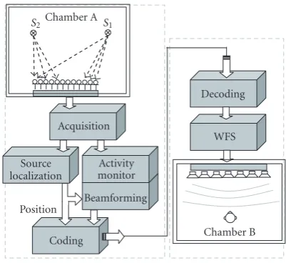
WFS Source
localization
Activity monitor Chamber A
S2 S1
Acquisition
Beamforming
Coding Position
Chamber B Decoding
Figure5: General architecture of the system.
localization. The full block diagram of the system can be seen inFigure 5.
The acquisition block receives the multichannel signals from the microphone array through a data acquisition (DAQ) board and captures digital audio samples to form multichannel audio streams.
Theactivity monitor basically consists in a vocal activ-ity detector that readjusts to the noise level and stops the adaptation process when necessary to avoid the appearance of sound artifacts.
The source localization (SL) block uses both acoustical (steered response power-phase transform (SRP-PHAT)) and video (face tracking) algorithms to obtain a good estimation of the position of the source. This information is needed by the beamforming component and the WFS synthesis block.
The beamforming algorithm employs a robust gener-alized sidelobe canceller (RGSC) scheme. For the adap-tive algorithms several alternaadap-tives have been tested in-cluding constrained-NLMS, frequency domain adaptive fil-ters (xFDAF), and conjugate gradient (CG) algorithms to achieve a good compromise between computational com-plexity, convergence speed, and latency.
Thecodingblock codifies the signal using two standard perceptual coders (MPEG2-AAC or G.722) to prove the com-patibility between the estimation process and the use of stan-dard codecs.
Finally, the acoustic field is rendered again in the receiv-ing room usreceiv-ing WFS techniques and a 10-loudspeaker array. Next sections give more details on the precise implementa-tion of each of these blocks.
3. ACQUISITION
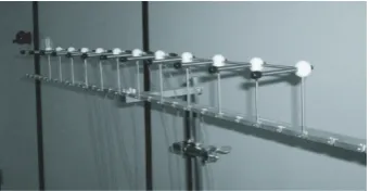
Figure6: Microphone array.
0 2000
4000
0
2000 4000
6000 0
500 1000 1500 2000 2500
y-position (mm) x-position (mm)
z
-position
(mm)
v46
v45
v44
v43
v42
v37
v36
v35
v34
v33
v32
v31
v27
v26
v25
v24
v23
v22
v21
v17
v16
v15
v14
v13
v12
v11
v06
v05
v04
v03
v02
Microphones
Figure7: Bell labs chamber.
of several parameters such as sampling frequency and No points to capture. The microphone array (Figure 6) has 12 linearly placed (8 cm separation) PCB Piezotronics omni-directional microphones (for our tests only eight were em-ployed) with included preamplifiers. The test signals were recorded at midnight to avoid disturbing ambient sounds like the air conditioned system.
As the chamber used in our tests shows low reverberation (RT60 <70 ms), to obtain the microphone signals we have also used some impulse response recordings of a varechoic chamber in Bell Labs [12] which offers higher reverberation values (RT60=380 ms). In that case the IRs were recorded from different audio locations (Figure 7) using a 22-linear omnidirectional microphone array (10 cm separation).
4. BEAMFORMING
4.1. Current beamforming alternatives
The spatial properties of microphone arrays can be used to improve or enhance the captured speech signal. Many adap-tive beamforming methods have been proposed in the lit-erature. Most of them are based on the linearly constrained minimum variance (LCMV) beamformer [11] which is often implemented using the generalized sidelobe canceller (GSC) developed by Griffiths and Jim [13]. The GSC (Figure 8) is based on three blocks: a fixed beamformer (FB) that en-hances the desired signal using some kind of delay-and-sum
n τ n
FB
d(n)
τ d
¼(
n) e(n)
n 1
n 1
BM MC
Figure8: GSC block diagram.
strategy (and the direction of arrival (DOA) estimation pro-vided by the SL block), the blocking matrix (BM) that blocks the desired signal and produces the noise/interference-only reference signal, and the multichannel canceller (MC) which tries to further improve the desired signal at the output of the FB using the reference provided by the BM.
The GSC scheme can obtain a high interference reduc-tion with a small number of microphones arranged on a small space. However, it suffers from several drawbacks and a number of methods to improve the robustness of the GSC have been proposed over the last years to deal with the array imperfections.
Probably, the biggest concern with the GSC is related to its sensibility to steering errors and/or the effect of reverber-ation. Steering-vector errors often result in target signal leak-age into the BM output. The blocking of the target signal be-comes incomplete and the output suffers from target signal cancellation. A variety of techniques to reduce the impact of this problem has been proposed. In general, these systems re-ceive the name of robust beamformers. Most approaches try to reduce the target signal leakage over the blocking matrix using different strategies. The alternatives include inserting multiple constraints in the BM to reject signals coming from several directions [14], restraining the coefficient growth in the MC to minimize the effect that eventual BM-leakage could cause [15], or using an adaptive BM [16] to enhance the blocking properties of the BM. Some recent strategies go even further, introducing a Wiener filter after the FB to try to obtain a better estimation [17]. Most implementations use some kind of voice activity detector [18] to stop the adap-tation process when necessary and avoid the appearance of sound artifacts.
Apart from dealing with target signal cancellation, there are some other key elements to take into account for our ap-plication.
(i) Convergence speed. In a quick time varying environ-ment, where small head movements of the speaker can change the response of the filter that we have to syn-thesize, the algorithm has to converge, necessarily, in a short period of time.
(ii) Computational complexity. The application is ori-ented towards building effective real-time communi-cation systems so efficient use of computational re-sources has to be taken into account.
Table1
NLMS FDAF PBFDAF CG Processing time (s) <0.70 <0.09 <0.19 >5 s Latency (samples) 1 128 32 1
The convergence speed problem is related to the kind of al-gorithm employed in the adaptive filters. Originally, typical GSC schemes use some kind of LMS filters due to its low computational cost. This algorithm is very simple but it suf-fers from not-so-good convergence time, so some GSC im-plementations use affine projection algorithms (APA) [19], conjugate gradient techniques [20, 21], or wave domain adaptive filtering (WDAF) [22] which speed up the conver-gence time at the cost of increasing the computational com-plexity. This parameter can be reduced using subband ap-proaches [23], with efficient complex valued arithmetic [24] or operating in the frequency domain (FDAF) [25,26].
4.2. Beamformer design: RGSC with mPBFDAF for MC
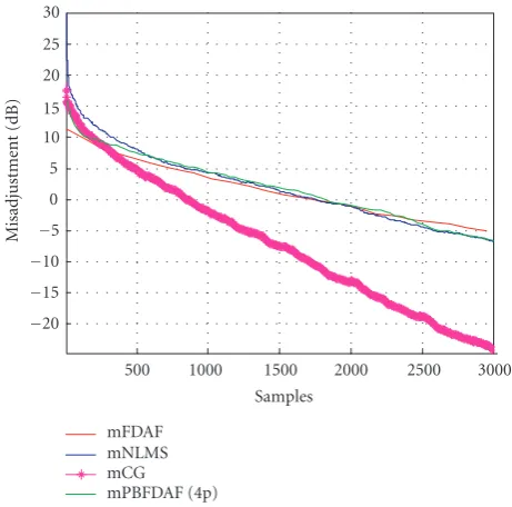
Figure 10shows our current implementation which uses the adaptive BM approach to reduce the target signal cancel-lation problem and a VAD to control the adaptation pro-cess. After considering several alternatives we decided to develop multichannel partitioned block frequency domain adaptive filters (mPBFDAF) [27] for the MC (as they show a good tradeoffbetween convergence speed, complexity, and latency) and a constrained version of a simple NLMS fil-ter for the BM. Subband conjugate gradient algorithms [28] were also tested but, although they showed really good con-vergence speed, they were discarded due to the enormous computational power they needed (two orders of magnitude higher compared to FDAF implementations, seeTable 1and
Figure 9).
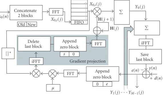
4.2.1. mPBFDAF (multichannel canceller)
PBFDAF filters take advantage of working in the frequency domain greatly reducing the computational complexity. Moreover, the filter partitioning strategy reduces the over-all latency of the algorithm making it very suitable for our interests.
Figure 11shows the multichannel implementation of the PBFDAF filter that we have developed for using in the MC. Assuming a filter with a long impulse responseh(n), it can be sectioned inLadjacent, equal length, and non-overlapping sections as
hk(n)= L 1
l=0
hk,l(n), (2)
wherehk,l(n)=hk(n) forn=lN,. . .,lN+N1,Lthe num-ber of partitions,kthe channel number (k=0,. . .,M1), andNthe length of the partitioned filter. This can be seen as a bank of parallel filters working in the full spectrum of the input signal.
500 1000 1500 2000 2500 3000 20
15 10 5 0 5 10 15 20 25 30
Samples
M
isadjust
m
ent
(dB)
mFDAF mNLMS mCG mPBFDAF (4p)
Figure 9: Convergence speed. System identification problem: 3 channels, 128 tap filters (PBFDAF using 4 partitionsL=4,N=32).
The output,y(n), can be obtained as the sum ofLparallel
N-tap filters with delayed inputs:
yk(n)=xk(n) L 1
l=0
hk,l(n)= L 1
l=0
xk(n)hk,l(n)
= L 1
l=0
xk(nlN)hk,l(n+lN)= L 1
l=0
yk,l(n). (3)
This way, using the appropriate data sectioning procedure theLlinear convolutions (per channel) of the filter can be independently carried in the frequency domain with a total delay ofNsamples instead of theNLsamples needed in stan-dard FDAF implementations.
After a signal concatenation block (2N-length blocks, necessary for avoiding undesired overlapping effects and to assure a mathematical equivalence with the time domain lin-ear convolution), the signal is transformed into the frequency domain. The resulting frequency block is stacked in a FIFO memory at a rate ofN samples. The final equivalent time output (with the contributions of every channel) is obtained as
y(n)=IFFT M 1
k=0 L 1
l=0
Xlk(jl)H l k
, (4)
where “j” represents the time index. Notice that we have al-tered the order of the final sum and IFFT operations as
IFFT M 1
k=0 L 1
l=0
Xlk(jl)H l k
= M 1
k=0 L 1
l=0
IFFTXlk(jl)H l k
.
x0(n)
xM 1(n)
BM
τ1
τ2
τM
τP
τP
τP
FB
d(n)
cNLMS0
cNLMS1
cNLMSM 1
x0(n P)
xM 1(n P)
τL
x¼
0(n)
x¼
1(n)
x¼
M 1(n)
d¼(
n)
..
.
PBFDAF0
PBFDAF1
PBFDAFM 1
e(n)
FFT
iFFT
Y0(w)
Y1(w)
YM 1(w)
Y(w)
MC
+
+
+
+
d(n)
x¼
0(n)
P
P Thresholdλ
Adaptation control
Comparator
Activity monitor .
. .
. . .
Figure10: General diagram RGSC implementation.
This way, we save (N1)(M1) FFT operations in the complete filtering process.
As in any adaptive system the error can be defined as
e(n)=d(n)y(n). (6)
On the other hand, as the filtering operation is done in the frequency domain, the actualization of the filter coefficients is performed in every frequency bin (i=0,. . ., 2N1)
Hkl,i(j+ 1)=Hkl,i(j)
+μl k,i(j) Prj
Ei(j)
Xk,i(jl+ 1)
£
, (7)
whereEiis the corresponding frequency bin, the asterisk de-notes complex conjugation, andμlk,idenotes the adaptation step. The “Prj” gradient projection operation is necessary for implementing the constrained version of the PBFDAF. This version adds two FFTs more (seeFigure 11) to the computa-tional burden but speeds up the convergence.
Finally, the adaptation step is computed using the spec-tral power information of the input signal:
μl k,i(j)=
u γ+ (L+ 1)Pki(j)
, (8)
whereurepresents a fixed step size parameter,γa constant to prevent the updating factor from getting too large, andPthe power estimate of theith frequency bin:
Pi
k(j)=λPki(j1) + (1λ)Xk,i(j) 2
. (9)
Beingλa small factor for the updating equation for the signal energy in the subbands.
4.2.2. cNLMS (blocking matrix)
Concatenate 2 blocks
x0(n)
Old New
FFT
X0,i(j) FIFO
X0,i(j)
H(j+ 1)
H(j)
Y0(j)
iFFT Save last block
y(n)
d(n)
e(n)
+
Y1(j)YM 1(j)
Append zero block
0 e
FFT
μ
iFFT Delete last block []
Append zero block
s 0
FFT
Gradient projection
Figure11: PBFDAF implementation.
adaptation process can be described as
h¼
n(j+ 1)=hn(j) +μ x ¼ n(j) d(j)Td(j)d(j),
hn(j+ 1)=
⎧ ⎪ ⎪ ⎪ ⎪ ⎨ ⎪ ⎪ ⎪ ⎪ ⎩
φn forh
¼
n(j+ 1)> φn,
ψn forh
¼
n(j+ 1)< ψn, h¼
n(j+ 1) otherwise,
(10)
where ψn and φn represent the lower and upper vector bounds for coefficients.
4.2.3. Activity monitor
The activity monitor is based on the measure of the local power of the incoming signals and tries to detect the pauses of the target speech signal. The MC weightings are estimated only during pauses of the desired signal and the BM weight-ings during the rest of the time. Basically, the pause detection is based on the estimation of the target signal-to-interference ratio (SIR). We are using the approach presented in [29] where the power ratio between the FB output and one of the outputs of the BM is compared to a threshold.
4.3. Source separation evaluation results
The full RGSC algorithm has been implemented in Mat-lab andC and runs in real time (8 channels, Fs = 16 kHz, BM = 32 taps, MC = 256 taps) in a 3.2 GHz Pentium IV. The behavior of the adaptive algorithm was tested in a real environment.
Two signals (Fs = 16 kHz, 4 s excerpts) were placed in positions v21 (speech signal) and v27 (white noise) (see
Figure 7) to see the performance of the algorithm in recov-ering the original dry speech signal.
Figure 12shows the SNR gain of each algorithm once the convergence time is over. The RGSC uses 16 tap filters at BM and 128 or 256 at the MC (2 configurations). As expected the longer the filter at the MC is, the better the results are; at SNR (input)=5 dB more than 20 dB of gain is achieved in
0 2 4 6 8 10 12 14 16 18 20
Input SNR (dB) 8
10 12 14 16 18 20 22 24
SNR
gain
(dB)
RGSC (256) FB RGSC (128)
10 channels
Figure12: SNR gain versus input SNR using 10 microphones.
contrast with the mere 9 dB gain with a standard fixed beam-former.
5. SOURCE LOCALIZATION
As mentioned in previous sections, source localization is nec-essary in the source separation process as well as in the sound field rendering process. From an acoustical point of view, there are three basic strategies when dealing with the source localization problem. Steered response power (SR) locators basically steer the array to various locations and search for a peak in the output power [30]. This method is highly depen-dant on the spectral content of the source signal; many im-plementations are based on a priori knowledge of the signals involved in the system making the scheme not very practical in real speech scenarios.
demanding as the SR methods but tend to be less robust when working with wideband signals although some recent work has tried to address this issue [32].
Finally, time-difference-of-arrival- (TDOA-) based lo-cators use time delay estimation (TDE) of the signals in different microphones usually employing some version of the generalized cross correlation (GCC) function [33]. This approach is computationally undemanding but suffers in high reverberant environments. This multipath channel dis-tortion can be partially solved making the GCC function more robust using a phase transform (PHAT) [34] to de-emphasize the frequency dependant weightings.
We have decided to use the SRP-PHAT method described in [35] that combines the inherent robustness of the steered response power approach with the benefits of working with PHAT transformed signals. The method is quite simple and starts with the computation of the generalized cross correla-tions between every microphone-pair signals:
R12(τ)= 1 2π
½
½
ψ12(ω)X1(w)X £
2(w)ejwτdω, (11)
whereX1(ω) andX2(ω) represent the signals in the micro-phones 1 and 2 andψ12the PHAT weighting defined by (12). The PHAT function emphasizes the GCC function at the true DOA values over the undesirable local maximums and improves the accuracy of the method,
ψ12(ω)= 1 X1(w)X£
2(w).
(12)
After computing the GCC of each microphone pair, as in any steered response method, a search between potential source location starts. For every location under test, the theoretical delays of each microphone pair have been previously calcu-lated. Using those delay values, for each position, the con-tribution of cross correlations is accumulated. The position with the highest score is chosen.
Figure 13 shows the method in action. Using the Bell chamber environment, a male speech (Fs =16 kHz, 4 s ex-cerpt, 8 microphones28 pairs) was placed in v46. Candi-date positions were selected using a 0.01 m2resolution. Fig-ures13(a)and13(b)(2D projection) show the result of run-ning the SRP-PHAT algorithm (whiterhigher values, win-dow512 taps 30 ms) where the “+” symbol marks the correct position and the “” the estimated one. As you can see, in these single speaker situations the DOA estimation is good but the problems arise when working in multiple source environments. In the test shown inFigure 13(c)a sec-ond (white noise) source was placed in v42 and the algorithm clearly had problems to identify the target source location. In those heavy competing noise situations acoustical methods (especially SRP-PHAT) suffer from high degradation.
To circumvent this problem we have used a second source of information: video-based source localization. Video-based source localization is not a new concept and has been exten-sively studied, especially in three-dimensional computer vi-sion [36]. Recently, we have seen an effort to mix the audio and video information for building robust location systems in low SNR environments. Those systems relay on Kalman
filtering [37] or Bayesian networks [38] for effective data fu-sion. We propose a very simple approach where video lo-calization is used as a first rough estimation that basically discards nonsuitable positions. The remaining potential lo-cations are tested using the SRP-PHAT algorithm in what we could call a visually guided acoustical source localization system. This position-pruning scheme is, most of the time, enough for rejecting problematic second source situations. Besides, the computational complexity associated to video signal processing is somehow compensated with a smaller search space for the SRP-PHAT algorithm.
Our video source location system is a real-time face tracker using detection of skin-color regions based on the machine perception toolbox (MPT) [39]. A sample result of face detection can be seen inFigure 14.
6. CODING/DECODING
After the estimation process, the signal must be codified prior to be sent. We have tested two different codification schemes, MPEG2-AAC (commonly used for wideband audio) and G-722 (very used in teleconference scenarios), to see if the es-timation process has any impact in the behavior of these al-gorithms. Luckily, in the informal subjective test comparing the original estimated signal (the same work situation as in
Section 4) with the coded/decoded signal (Figure 15), the lis-teners were unable to distinguish between both situations neither when using AAC (64 kbps/channel) nor when work-ing with G.722 (64 kbps/channel).
7. WAVE FIELD SYNTHESIS
The last process involves rebuilding the acoustic field again at reception. The sound field rendering process is based on well-known WFS techniques. We are using a 10-loudspeaker array situated in a different chamber than the ones used for signal capturing. The synthesis algorithm is based on [40], although no room compensation was applied. Derivation of the driving signals for a line of loudspeakers is found in [41] and can be summarised with the expression:
Qrn,ω
=S(ω)cosθn
Gφn
jk
2π
1 2
e jkrn
rn
, (13)
whereQ(rn,ω) is the driving signal of the loudspeaker,S(ω) the virtual estimated source,θn the angle between the vir-tual source and the main axis of thenth loudspeaker, and
G(φn,ω) the directivity index of the virtual source (omnidi-rectional in our tests). Also notice that no special method was applied to override the maximum spatial aliasing frequency problem (around 1 kHz). However, it seems [42] that the hu-man auditory system is not so sensitive to these aliasing arti-facts.
8. SUBJECTIVE EVALUATION
0
1000 2000
3000 4000
5000 6000 70005000 4000
3000 2000
1000
x
y
0 0.2 0.4 0.6
SRP
-P
H
A
T
val
u
e
Microphones
(a)
Clear DOA
+ 1000 2000 3000 4000 5000 6000 5000
4500 4000 3500 3000 2500 2000
x y
(b)
Error! 2 sources
+ +
1000 2000 3000 4000 5000 6000 5000
4500 4000 3500 3000 2500 2000
x y
(c)
Figure13: Source localization using SRP-PHAT. (a) Single source, (b) single source (2D projection), and (c) multiple sources.
Figure14: Face tracking.
MOS experiments have been carried out to see how well the system performed. Two signals, speech in v21 and white noise in v27 (SNRin = 5 dB), were recorded by the micro-phone array in the emitting room. After the beamforming process the estimated signal was used to render again the
AAC/G.722 coder
AAC/G.722 decoder
COMP Estimated
source
Figure15: Comparison: estimated signal versus coded/decoded sig-nal.
Figure16: Loudspeaker array.
Low ref. FB RGSC128 RGSC256 Up ref. 0
20 40 60 80 100 120
M
ean
opinion
sc
o
re
(MUSHRA)
13.7
38.9
63.3
75
100
Figure17: Mean opinion score (MUSHRA test) after WFS.
codification schemes. Fifteen listeners took part in the test;
Figure 16shows the relative position of the subjects to the array (centred position distance: 1.5 m).
In this kind of tests, the listener is presented with all dif-ferent processed versions of the test item at the same time. This allows the subject to easily change between different ver-sions of the test item and to come to a decision about the relative quality of the different versions. The original, unpro-cessed version (identified as the reference version) of the test item is always available to the subject to give him the idea how the item should really sound. In our case, the reference version was the sound field recreated (via WFS) using the original dry signal (as if all the noise had disappeared and the estimation of the source was perfect). This version is also presented to the subject as a hidden upper reference to ensure that the top of the scale is used. On the other side, to ensure that the low part of the scale is used, the standard proposes to employ a 3.5 kHz filtered version of the original reference which is not applicable to our situation as it lacks from the effect of the ambient noise. In our case we decided to use the sound field rendered using the sound captured by the central microphone of the array (without any noise reduction). We refer to this version as the hidden lower reference. Using both hidden anchors, we ensure that the full range of the scale is used and the system obtains more realistic values.
The subjects are required to assign grades giving their opinion of the quality under test and the hidden anchors. In
our case, the subjects were instructed to pay special atten-tion not only to overall quality, intelligibility, signal cancella-tion, or sound artifact appearance but they were also asked to concentrate on any displacements of the localization of the source. Any source movement should obtain a low score. The scale is numerical and goes from 100 to 0 (100–80: ex-cellent, 80–60 good, 60–40 fair, 40–20 poor, 20–0 bad). Sub-jects were instructed to score 30 audio excerpts (6 different sentences, 5 situations per sentence: hidden upper reference, RGSC (256 taps in the MC), RGSC (128), fixed beamformer, hidden lower reference). The original dry sentences were se-lected from the Albayzin speech database [45] (Fs=16 kHz, Spanish language). As the way the instructions are given to the listeners can significantly affect the way a subject per-forms the test, all the listeners were instructed the same way (using a 2-page documentation).
The results are shown inFigure 17where the number on each bar represents the mean score obtained by each method and the vertical hatched box indicates a 95% confidence interval. Nearly all the listeners were able to describe the de-sired source coming from the right position and almost none of them described any target signal cancellation or the ap-pearance of disturbing sound artifacts.
9. CONCLUSIONS AND FUTURE WORK
In this paper we have seen some of the challenges that fu-ture immersive audio applications have to deal with. We have presented a range of solutions that behave quite well in nearly every area. Partitioned block frequency domain-based robust adaptive beamforming significantly enhances the speech sig-nals at the same time that keeps low computational require-ments allowing a real time implementation.
On the other side, visually guided acoustical source local-ization is capable of dealing with not-so-low reverberation chambers and multiple source situations and provides with good localization estimations both the beamforming block and the WFS block. The WFS-based rendered acoustical field shows good spatial properties as the MUSHRA-based sub-jective tests have assessed. However, there is margin for im-provement in many areas.
ACKNOWLEDGMENTS
This work was supported by project PCT-350100-04 and by Spanish Science and Technology Department through projects TIC 2003-09061-c03-01 and “Ramon y Cajal.” The authors would also like to thank Mariano Garc´ıa for his valu-able comments.
REFERENCES
[1] A. Blumlein, “Improvements in and relating to sound trans-mission, sound-recording and sound reproduction systems,” patent no. 394325 December 1931.
[2] W. B. Snow, “Basic principle of stereophonic sound,”Journal of SMPTE, vol. 61, pp. 567–589, 1953.
[3] W. B. Snow, “Auditory perspective,”Bell Laboratories Record, vol. 12, pp. 194–198, 1934.
[4] A. H¨arm¨a, “Coding principles for virtual acoustic openings,” inProccedings of the Audio Engineering Society 22nd Conference on Virtual, Synthetic and Entertainment Audio (AES22 ’02), pp. 159–165, Espoo, Finland, June 2002.
[5] S. Torres, J. A. Beracoechea, I. P´erez-Garc´ıa, et al., “Coding strategies and quality measure for multichannel audio,” in Pro-ceedings of the 116th Audio Engineering Society Convention, Berlin, Germany, May 2004.
[6] H. Teutsch, S. Spors, W. Herbordt, W. Kellermann, and R. Rabesnstein, “An integrated real-time system for immersive audio aplications,” inProceedings of IEEE Workshop on Appli-cations of Signal Processing to Audio and Acoustics (WASPAA ’03), New Paltz, NY, USA, October 2003.
[7] W. Kellermann, “Acoustic signal processing for next gener-ation human/machine interfaces,” in Proceedings of the 8th International Conference on Digital Audio Effects (DAFx ’05), Madrid, Spain, September 2005.
[8] A. J. Berkhout, “Holographic approach to acoustic control,” Journal of the Audio Engineering Society, vol. 36, no. 12, pp. 977–995, 1988.
[9] M. M. Boone and W. P. J. Bruijn, “Improving speech intelli-gibility in teleconferencing by using Wave Field Synthesis,” in Proceedings of the 114th Audio Engineering Society Convention, Amsterdam, The Netherlands, March 2003.
[10] W. P. J. Bruijn and M. M. Boone, “Application of Wave Field Synthesis in life-size videoconferencing,” inProceedings of the 114th Audio Engineering Society Convention, Amsterdam, The Netherlands, March 2003.
[11] B. D. Van Veen and K. M. Buckley, “Beamforming: a versa-tile approach to spatial filtering,”IEEE ASSP magazine, vol. 5, no. 2, pp. 4–24, 1988.
[12] Bell Labs’s Varecoic Chamberhttp://www.bell-labs.com/org/ 1133/Research/Acoustics/VarechoicChamber.html.
[13] L. J. Griffiths and C. W. Jim, “Alternative approach to linearly constrained adaptive beamforming,”IEEE Transactions on An-tennas and Propagation, vol. 30, no. 1, pp. 27–34, 1982. [14] B. Widrow and J. M. McCool, “Comparison of adaptive
al-gorithms based on the methods of steepest descent and ran-dom search,”IEEE Transactions on Antennas and Propagation, vol. 24, no. 5, pp. 615–637, 1976.
[15] Y. Liu, Q. Zou, and Z. Lin, “Generalized sidelobe cancellers with leakage constraints,” inProceedings of IEEE International Symposium on Circuits and Systems (ISCAS ’05), Kobe, Japan, May 2005.
[16] O. Hoshuyama, A. Sugiyama, and A. Hirano, “Robust adaptive beamformer for microphone arrays with a blocking matrix
using constrained adaptive filters,”IEEE Transactions on Sig-nal Processing, vol. 47, no. 10, pp. 2677–2684, 1999.
[17] A. Abad and J. Hernando, “Integrated adaptive beamform-ing and Wiener filterbeamform-ing for a robust microphone array,” in IEEE Sensor Array and Multichannel Signal Processing Work-shop (SAM ’04), pp. 367–371, Barcelona, Spain, July 2004. [18] Z. M. Saric and S. T. Jovicic, “Adaptive microphone array
based on pause detection,”Acoustic Research Letters Online, vol. 5, no. 2, pp. 68–74, 2004.
[19] Y. Zheng and R. Goubran, “Adaptive beamforming using Affine Projection Algorithms,” in Proceedings of 5th Inter-national Conference on Signal Processing (ICSP ’00), Beijing, China, August 2000.
[20] J. A. Apolin´ario Jr., M. L. R. De Campos, and C. P. O. Bernal, “Constrained conjugate gradient algorithm,”IEEE Signal Pro-cessing Letters, vol. 7, no. 12, pp. 351–354, 2000.
[21] J. A. Beracoechea, S. Torres, L. Garc´ıa, et al., “Source sepa-ration for microphone arrays using conjugate gradient tech-niques,” inProceedings of the 8th International Conference on Digital Audio Effects (DAFx ’05), Madrid, Spain, September 2005.
[22] H. Buchner, S. Spors, and W. Kellermann, “Wave-domain adaptive filtering: acoustic echo cancellation for full-duplex systems based on wave-field synthesis,” inProceedings of IEEE International Conference on Acoustics, Speech and Signal Pro-cessing (ICASSP ’04), vol. 4, pp. 117–120, Montreal, Quebec, Canada, May 2004.
[23] S. Low, S. Nordholm, and N. Grbic, “Subband generalized Sidelobe approach—a constrained region approach,” in Pro-ceedings of IEEE Workshop on Applications of Signal Processing to Audio and Acoustics (WASPAA ’03), New Paltz, NY, USA, October 2003.
[24] G. Glentis, “Implementation of adaptive generalized side-lobe cancellers using complex valued arithmetic,” Interna-tional Journal of Applied Mathematics and Computer Science, vol. 13, no. 4, pp. 549–566, 2003.
[25] W. Herbordt and W. Kellermann, “Efficient frequency-domain realization of robust generalized sidelobe cancellers,” in Pro-ceedings of IEEE 4th Workshop on Multimedia Signal Processing, pp. 377–382, Cannes, France, October 2001.
[26] Z. L. Yu and M. H. Er, “An extended generalized sidelobe can-celler in time and frequency domain,” inProceedings of IEEE International Symposium on Circuits and Systems (ISCAS ’05), vol. 3, pp. 629–632, Vancouver, BC, Canada, May 2004. [27] J. M. P´aez Borrallo and M. Garc´ıa Otero, “On the
implemen-tation of a partitioned block frequency domain adaptive filter (PBFDAF) for long acoustic echo cancellation,”Signal Process-ing, vol. 27, no. 3, pp. 301–315, 1992.
[28] L. Garc´ıa, S. Torres, J. A. Beracoechea, et al., “Conjugate Gra-dient techniques for Multichannel acoustic echo cancellation,” inProceedings of the 8th International Conference on Digital Audio Effects (DAFx ’05), Madrid, Spain, September 2005. [29] O. Hoshuyama, B. Begasse, A. Sugiyama, and A. Hirano,
“Re-altime robust adaptive microphone array controlled by an SNR estimate,” inProceedings of IEEE International Conference on Acoustics, Speech and Signal Processing (ICASSP ’98), vol. 6, pp. 3605–3608, Seattler, Wash, USA, May 1998.
[30] N. Strobel, T. Meier, and R. Rabenstein, “Speaker localiza-tion using a steered filter-and-sum beamformer,” inErlangen Workshop ’99: Vision, Modeling and Visualization, Erlangen, Germany, November 1999.
[31] S. Haykin,Adaptive Filter Theory, Prentice Hall, Englewood Cliffs, NJ, USA, 1991.
inProceedings of IEEE International Conference on Acoustics, Speech, and Signal Processing (ICASSP ’05), Philadelphia, Pa, USA, March 2005.
[33] C. H. Knapp and G. C. Carter, “Generalized correlation meth-od for estimation of time delay,”IEEE Transactions on Acous-tics, Speech, and Signal Processing, vol. 24, no. 4, pp. 320–327, 1976.
[34] H. Wang and P. Chu, “Voice source localization for automatic camera pointing system in videoconferencing,” inProceedings of IEEE International Conference on Acoustics, Speech and Sig-nal Processing (ICASSP ’97), vol. 1, pp. 187–190, Munich, Ger-many, April 1997.
[35] J. DiBiase, H. Silverman, and M. Brandstein, “Robust local-ization in reverberant rooms,” inMicrophone Arrays; Signal Processing Techniques and Applications, pp. 157–180, Springer, Berlin, Germany, 2001.
[36] O. Faugeras,Three-Dimensional Computer Vision. A Geometric Viewpoint, MIT press, Cambridge, Mass, USA, 1993. [37] N. Strobel, S. Spors, and R. Rabenstein, “Joint audio-video
signal processing for object localization and tracking,” in Mi-crophone Arrays: Signal Processing Techniques and Applications, M. S. Brandstein and D. B. Ward, Eds., pp. 197–219, Springer, Berlin, Germany, 2001.
[38] F. Asano, K. Yamamoto, I. Hara, et al., “Detection and separa-tion of speech event using audio and video informasepara-tion fusion and its application to robust speech interface,”EURASIP Jour-nal on Applied SigJour-nal Processing, vol. 2004, no. 11, pp. 1727– 1738, 2004.
[39] I. Fasel, B. Fortenberry, and J. Movellan, “A generative frame-work for real-time object detection and classification,” Com-puter Vision and Image Understanding, vol. 98, pp. 182–210, 2005.
[40] S. Bleda, J. J. L ´opez, and B. Pueo, “Software for the simulation, performance analysis and real time implementation of Wave Field Synthesis systems for 3D Audio,” inProceedings the 6th International Conference on Digital Audio Effects (DAFx ’03), London, UK, September 2003.
[41] D. De Vries, “Sound reinforcement by wavefield synthesis: adaptation of the synthesis operator to the loudspeaker direc-tivity characteristics,”Journal of the Audio Engineering Society, vol. 44, no. 12, pp. 1120–1131, 1996.
[42] M. M. Boone, “Acoustic rendering with wave field systhesis,” inProceedings of the ACM Siggraph and Eurographics Camp-fire on Acoustic Rendering for Virtual Environments, pp. 37–45, Snowbird, Utah, USA, May 2001.
[43] MUSHRA (MUlti Stimulus test with Hidden Reference and Anchor, ITU-R BS.1534).
[44] ITU-R BS.1116-1, “Methods for the subjective assessment of small impairments in audio systems including multichannel sound systems”.
[45] Albayzin. Spanish Speech Database. Universidad Polit´ecnica de Catalu˜na. Proyecto TIC91-1488-C06.
[46] S. Spors, H. Buchner, and R. Rabenstein, “A novel approach to active listening room compensation for wave field synthe-sis using wave-domain adaptive filtering,” inProceedings of IEEE International Conference on Acoustics, Speech and Signal Processing (ICASSP ’04), vol. 4, pp. 29–32, Montreal, Quebec, Canada, May 2004.
J. A. Beracoecheareceived the Telecom En-gineer degree from Universidad Europea de Madrid (UEM) in 2001. He is currently working towards the Ph.D. degree at the Signal Processing Group at the Universi-dad Polit´ecnica de Madrid (UPM). His re-search interests include multichannel au-dio coding, microphone and loudspeaker arrays, beamforming, and source tracking with particular emphasis on the application
of the virtual acoustic opening for creating immersive audio sys-tems.
S. Torres-Guijarroreceived the M.Eng. and Ph.D. degrees in telecommunication engi-neering from the Universidad Polit´ecnica de Madrid, Spain, in 1992 and 1996, respec-tively. Dr. Torres worked as a teacher at the Universidad de Valladolid, Universidad Car-los III de Madrid, and Universidad Europea de Madrid. Since 2002 she has been work-ing as a Researcher of the Ram ´on y Cajal program at the Universidad Polit´ecnica de
Madrid, first, and at the Universidad de Vigo, at the moment. Her main research interest includes digital signal processing applied to speech, audio, and acoustics.
L. Garc´ıareceived the Automatic Control Engineer degree from Instituto Superior Polit´ecnico JAE., Havana, Cuba, in 1985, the Signals, System, and Radiocommunication Masters and the Ph.D. degrees in technolo-gies and systems of communications from Universidad Polit´ecnica de Madrid, Spain, in 1994 and 2006, respectively. From 1986 to 1990 he was a Solution Developer in the Company of Development of Automated
Systems Direction of Cuban Industry Ministry. From 1991 to 1993 he was a Researcher and Professor of multimedia in Superior Art Institute of Havana, Cuba. From 1995 to 1997 he was a Re-searcher in the Spanish Council for Scientific Research. From 1999 to 2002 he was a Professor in the Universidad Pontificia Comillas of Madrid, Spain. Since 2003 he is a Professor in Universidad Europea de Madrid, Spain. His technical interests are in the areas of signal processing and artificial intelligence.
F. J. Casaj ´us-Quir ´os received the M.Eng. and Ph.D. degrees in telecommunica-tion engineering from the Universidad Polit´ecnica de Madrid (Technical University of Madrid), Spain, in 1982 and 1988, re-spectively. He has been an Associate Profes-sor in that University since 1989, where he is Vice-Head of the Signals, System, and Ra-diocommunications Department. His main research interests are in digital signal