R E S E A R C H
Open Access
A variable-parameter normalized mixed-norm
(VPNMN) adaptive algorithm
Azzedine Zerguine
Abstract
Since both the least mean-square (LMS) and least mean-fourth (LMF) algorithms suffer individually from the problem of eigenvalue spread, so will the mixed-norm LMS-LMF algorithm. Therefore, to overcome this problem for the mixed-norm LMS-LMF, we are adopting here the same technique of normalization (normalizing with the power of the input) that was successfully used with the LMS and LMF separately. Consequently a new normalized variable-parameter mixed-norm (VPNMN) adaptive algorithm is proposed in this study. This algorithm is derived by exploiting a time-varying mixing parameter in the traditional mixed-norm LMS-LMF weight update equation. The time-varying mixing parameter is adjusted according to a well-known technique used in the adaptation of the step-size parameter of the LMS algorithm. In order to study the theoretical aspects of the proposed VPNMN adaptive algorithm, our study also addresses its convergence analysis, and assesses its performance using the concept of energy conservation. Extensive simulation results corroborate our theoretical findings and show that a substantial improvement, in both convergence time and steady-state error, can be obtained with the proposed algorithm. Finally, the VPNMN algorithm proved its usefulness in a noise cancellation application where it showed its superiority over the normalized least-mean square algorithm.
Keywords:LMS algorithm, NLMS algorithm, LMF algorithm, mixed-norm algorithms, normalized mixed-norm algorithms
1 Introduction
Due to its simplicity, the least mean-square (LMS) [1,2] algorithm is the most widely used algorithm for adaptive filters in many applications. The least mean-fourth (LMF) [3] algorithm was also proposed later as a special case of the more general family of steepest descent algo-rithms [4] with 2k error norms, k being a positive integer.
But for both of these algorithms, the convergence behavior depends on the condition number, i.e., on the ratio of the maximum to the minimum eigenvalues of the input signal autocorrelation matrix, R=E[xnxTn]
where xnis the input signal. This is clearly seen from their respective time constants [1,3]
τiLMS=
1
μλi
, i= 0, 1,. . .,N−1, (1)
and
τiLMF=
1 6μσ2
ηλi
, i= 0, 1,. . .,N−1, (2)
whereση2is the noise power,liis theitheigenvalue of the autocorrelation matrix of the input signal,µ is the step size used in the adaptation scheme and N is the number of coefficients in the adaptive filter. As seen
from (1) and (2), the ratio of
τ
max
τmin
is constant for
both algorithms and is given by the eigenvalue spread
(i.e., condition number),λmax
λmin i.e.,
τmax
τmin
= λmax
λmin
. (3)
To remove the dependency of the convergence of the LMS algorithm on the condition number, the normal-ized least-mean square (NLMS) [5] was introduced. As reported in [5], a great improvement in convergence is Correspondence: [email protected]
Electrical Engineering Department, King Fahd University of Petroleum & Minerals, Dhahran 31261, Saudi Arabia
obtained through the use of the NLMS algorithm over that of the LMS algorithm at the expense of a larger steady-state error. Similar results were obtained for the case of the normalized LMF (NLMF) algorithm [6-8].
A mixed-norm algorithm [9-11], combining both the LMS and the LMF algorithms, will suffer as well from the problem of the eigenvalue spread dependency. Since both of these algorithms suffer individually from this problem, to circumvent this problem for the mixed-norm LMS-LMF, we are adopting here the same techni-que of normalization that was successfully used with the LMS and LMF separately.
It is well known that fast convergence and lower steady-state error are two conflicting parameters in general adap-tive filtering. When compared to the LMS algorithm, the NLMS algorithm results in a faster convergence but only at the expense of a higher steady-state error [12,13]. A promising solution to this conflict is a time-varying nor-malized norm LMS-LMF algorithm. In this mixed-norm algorithm and during the transient state, the NLMS algorithm is used to speed up the algorithm’s convergence. However when steady-state is reached, the algorithm auto-matically switches from the NLMS to the NLMF [7], thanks to a built-in“gear shifting”property, to secure a lower steady-state error.
In this work, the performance of a variable-parameter normalized mixed-norm (VPNMN) LMS-LMF algorithm is evaluated. It will be shown that a better performance in both convergence and steady-state error will be achieved by the VPNMN algorithm than either the NLMS or the NLMF algorithm.
The rest of the article is organized as follows. Section 2 deals with a more explicit development of the proposed algorithm, and Section 3 treats its convergence analysis. The steady-state analysis of the proposed algorithm is detailed in Section 4, while its tracking analysis is given in Section 5. Performance evaluation of the resulting algorithm is carried out in Section 6. Finally, the conclu-sion section summarizes this work.
2 Algorithm development
The mixed-norm LMS-LMF algorithm is based on the minimization of the following cost function [9,10]:
Jn=αE[e2n] + (1−α)E[e4n], (4)
whereais a positive mixing parameter in the interval [0, 1] and the errorenis defined as
en=dn+ηn−xTnwn, (5)
where dn is the desired value, wn is the filter coeffi-cient of the adaptive filter,xnis the input signal andhn is the additive noise.
A major drawback of this algorithm is, however, the choice of the mixing parameter that is hard to fix a priorifor an unknown system. In [14], a self-adapting LMS-LMF algorithm with a time-varying weighting fac-tor was proposed. This time-variation of the weighting factor was achieved by allowing for a variable mixing factor that is updated every iteration using the modified variable step-size (MVSS) algorithm proposed in [15]. The variable weight mixed-norm LMS-LMF algorithm was defined to minimize the following performance measure [14]:
Jn=αnE[e2n] + (1−αn)E[e4n], (6)
wherean, chosen in [0, 1] such that the unimodal char-acter of the above cost is preserved, is a time-varying parameter updated according to [15]
αn+1=δαn+γp2n, (7)
and
pn=βpn−1+ (1−β)enen−1. (8)
The parametersδandb, both confined to the interval [0,1], are exponential weighting parameters that govern the averaging time constant, i.e., the quality of estima-tion of the algorithm, andg>0. Note that the algorithm defined by (4) is restored when δ=1 andg= 0, which forcesanto have a fixed value.
Based on this motivation, the weight mixed-norm LMS-LMF algorithm for recursively adjusting the coeffi-cients of the system is expressed in the following form:
wn+1=wn+μ[αnen+ 2(1−αn)e3n]xn, (9)
whereμis the step size.
As mentioned earlier and because of its reliance on the LMS and the LMF, the algorithm defined by (9) will be affected by the eigenvalue spread of the autocorrela-tion matrix of the input signal. To overcome this depen-dency, a VPNMN adaptive algorithm is introduced and its weight update recursion is given by the following expression:
wn+1=wn+μ[αnen+ 2(1−αn)e3n]
xn
xn2
, (10)
where║xn║2is the Euclidean norm of the input signal
xn. In the case of zero input, the ε-VPNMN algorithm defined as follows:
wn+1=wn+μ[αnen+ 2(1−αn)e3n]
xn
ε+xn2
, (11)
3 Convergence analysis of the VPNMN algorithm
In this section, the convergence analysis of the proposed VPNMN algorithm is carried out. Both the mean and the mean-square behaviors of the weight error vector are presented in the ensuing analysis.
3.1 Mean behavior
In the ensuing analysis, the following assumptions are used in the derivations of the convergence in the mean for the normalized mixed-norm LMS-LMF algorithm. These are quite similar to what is usually assumed in lit-erature [2-4,16] and which can also be justified in sev-eral practical instances
A.1 The noise sequence {hn} is statistically indepen-dent of the input signal sequence {xn} and both sequences have zero mean.
A.2The weight error vector (vn), to be defined later, is independent of the inputxn.
A.3The mixing parameter is independent of both the input signal and the error.
Examining the mean behavior of (10) under the above assumptions, sufficient conditions for convergence of the proposed algorithm in-the-mean can be derived and are stated as follows.
Proposition 1For the algorithm defined by(10)to con-verge in-the-mean, a sufficient condition is thatμbe cho-sen in the following range:
0< μ < 2
¯
αn+ 3(1− ¯αn)(ση2+C)
, (12)
where ση2is the noise power, α¯n=E[αn]is the mean of
the mixing parameter, andCis is the Cramer-Rao bound associated with the problem of estimating the random quantityxT
nwoptby using xTnwn.
Proof:The mean convergence of the proposed
algo-rithm is now studied by taking the expectation of the weight error vector, vn= wn - wopt. In this regard, the
errorencan be set up in the following way:
en=ηn−xTnvn, (13)
and hence (10) becomes
vn+1=vn+μ[αnen+ 2(1−αn)e3n]
xn
xn2
. (14)
Consequently, taking the expectation on both sides of (14), underA.1-A.3, the mean weight-error vector of the proposed algorithm evolves as
E[vn+1] =E[vn] +μ
¯ αnE
en xn
xn2
+ (1− ¯αn)E
e3
n xn
xn2
. (15)
Now, considering the second expectation in the above equation, This will be especially true when the filter is
long enough. Consequently, the independence assump-tion can be invoked to obtain the following:
E
en xn
xn2
≈ E[enxn]
tr(R) . (16)
To solve the expectationE[enxn] we use the technique of [17], and thus it results in
E[enxn] =−tr(R)E[vn]. (17)
Now, considering the second expectation in the above equation, This will be especially true when the filter is long enough. Consequently, the independence assump-tion can be invoked to obtain the following:
E
e3n xn
xn2
≈ E[e3nxn]
tr(R) . (18)
To solve the expectationEe3nxn we use the technique
of [17,18], which does not employ any linearization ofe3
n
As a result,E[e3nxn]is found to be
E[e3nxn] =−3(ση2+ζn)RE[vn]. (19)
Ultimately, (15) can be set up in the following form:
E[vn+1]≈
I−μ
¯
αn+ 3(1− ¯αn)
(σ2 η +ζn)
tr(R) R
E[vn].(20)
IfC≤ζnis the Cramer-Rao bound associated with the
problem of estimating the random quantity xT nwoptby using xT
nwn, then after taking into account the fact that
the eigenvalues ofRare all real and positive,lmaxbeing
the largest eigenvalue of Rand in general lmax<tr(R)
[19], it follows that a sufficient condition for conver-gence of the proposed algorithm is that the step-size parameterμsatisfies (12).▪
Two extreme scenarios can be considered here for the value of the mixing parameteran
(1) Scenario 1: Whenan = 0, the VPNMN algorithm reduces to the NLMF algorithm [6], and it can be shown that (12) becomes
0< μ < 2
3(σ2 η +C)
. (21)
(2) Scenario 2: Whenan = 1, both the NLMS algo-rithm and its step size range, that is 0 < μ < 2, are recovered.
Remarks:
(1) It can be seen from (10) that the VPNMN algo-rithm can be viewed as a variable step-size LMS-LMF algorithm with time varying step size.
signal power,║xn║2, will act as a threshold to avoid taking large step sizes when the error converges to a minimum in the recursive updating equation.
(3) The bound for the step-size (μ) of the proposed algorithm that guarantees convergence of the mean weight-vector, given by (12), shows that the mean-weight-vector stability depends on the Cramer-Rao bound. Therefore, the convergence of the weight-vector of the proposed algorithm depends on its mean-square stability. A similar fact was observed in [18] for the LMF algorithm.
3.2 Mean square behavior
In this section the performance of the VPNMN algorithm in the mean-square sense is analyzed. Here, we have used a unified approach to the transient analysis of adaptive filters with error nonlinearities. This approach does not restrict the regression data to be Gaussian and avoids the need for explicit recursions for the covariance matrix of the weight-error vector. This approach assumes that the adaptive filter is long enough to justify the following assumptions which are realistic for longer adaptive filters: A.4 The residual or a priori error ean, to be defined
later, can be assumed to be Gaussian.
A.5 The norm of the input regressor (║xn║2) can be assumed to be uncorrelated withf2(en) (f(en) is defined in (23)).
The framework is based on the concept of energy con-servation relation which was first noted in [20] and in general the adaptation scheme defined in (14) can be written in the following form:
vn+1=vn+μxnf(en), (22)
wheref(en)denotes a general scalar function of the output estimation errorenand in our case it is given by
f(en) = αnen+ 2(1−αn)e
3
n
xn2
. (23)
We are interested in studying the time-evolution and the steady-state values of E[|e2
an|]and E[║vn║2] which represent the error and the mean-square-deviation performances of the filter, respectively, whereas their time-evolution relate to the learning or the transient behavior of the filter.
Then, for some symmetric positive definite weighting matrixAto be specified later, the weighteda prioriand a posteriori estimation errors are, respectively, defined as [21]
eAan=xTnAvn, and eApn =xTnAvn+1. (24)
For the special case whenA=I, the weighteda priori and a posteriori estimation errors defined above are
reduced to standard a priorianda posterioriestimation errors, respectively, that is,
ean=eIan=x T
nvn, and epn=eIpn=x T
nvn+1. (25) It can be shown that the estimation error, en, and the a priori error, ean, are related via en= ean +hn. Also, using (10) and (24), it can be shown that
eApn=eAan− xn2Aμf(en), (26)
where the notation xn2A denotes the weighted
squared Euclidean normxn2A=xTnAxn.
The performance measure in the analysis is the excess mean-square-error (EMSE), denoted by ζn, and is defined as follows:
ζn=E[|en|2]−ση2. (27)
Sinceean=xTnvn, the EMSE can also be written as
fol-lows:
ζn=E[|ean|2] =E[vn2R|.
(28)
Next, the fundamental weighted-energy conservation relation given in [21] is presented to develop the frame-work for the transient analysis of the proposed algo-rithm. Thus, by substituting (26) in (22), the following relation can be obtained:
vn+1=vn−
xn
xn2A
[eAan−eApn]. (29)
Ultimately, the fundamental weighted-energy conser-vation relation can be shown to be
vn+12A+ 1
xn2A
|eAan|2=vn2A+ 1
xn2A
|eApn|2. (30)
This relation shows how the weighted energies of the error quantities evolve in time. It has been shown that different choices ofAallow us to evaluate different per-formance measures of an adaptive filter.
3.2.1 Time evolution of the weighted varianceE[vn2A]
In this section, the time evolution of the weighted var-iance E[vn2A]is derived for the proposed algorithm
using the fundamental weighted-energy conservation relation (30). Substituting the expression fora posteriori error from (26) in (30) and taking expectation on both sides to obtain the following relation:
E[vn+12A] =E[vn2A]−2μE[eAanf(en)] +μ2E[xn2Af2(en)]. (31)
Now, evaluating the two expectations in second and third terms on the right hand side of the above equa-tion, that is,E[eA
for these two quantities are given next. First, we will use the following assumption which was adopted in [21], that is,
A.6For any constant matrix Aand for all n, ean and
eAanare jointly Gaussian.
This assumption is reasonable for longer filters using the concept of central limit arguments [21]. Moreover, a similar assumption was used in [22]. Hence, we can sim-plify the expectation E[eA
anen]using Price’s Theorem
[23,24] and assumptionsA.4andA.6 asfollows:
E[eAanf(en)] =E[eAanf(en)]
=E[eAanean]
E[eanf(en)] E[e2
an]
. (32)
SinceeAan=xTnAvnandean=xTnIvnwe can simplify the
expectationE[eA
anean]as follows:
E[eAanean] =E[xTnAvnxTnIvn] =E[vn2AxT
nxnI]
=E[vn2AR].
(33)
Ultimately, (32) can be written as
E[eAanf(en)] =E[vn2AR]
E[eanf(en)]
E[eA
an]
. (34)
The term E[eanf(en)]
E[e2 an]
for the case of proposed
algo-rithm, can be shown to be
E[eanf(en)]
E[e2 an]
= 1
N
¯
αn+ 6(1− ¯αn)(ζn+ση2) ,
–Zn.
(35)
Second, to solve the expectationE[xn2Af2(en)], we
will resort to the following assumption [21]:
A.7 The adaptive filter is long enough such that xn2Aandf
2
(en) are uncorrelated.
This assumption is found to be more realistic as the fil-ter gets longer [21] and unweighted version of this assumption was used in [22,25]. The assumption enable us to split the expectationE[xn2Af2(en)]as follows:
E[xn2Af2(en)] =E[xn2A]E[f2(en)], (36)
whereE[f2(en)] can be shown to be (withα2
n =E[αn2])
E[f2(e
n)] =1
N2
α2
n(ζn+σ2
η) + 60(1−2¯αn+α2
n)(ζn+σ2
η)3+ 4(¯αn−α2n)(3ζn2+ 6ζnση2+ 3ση2),
Fn. (37)
Ultimately, we can rewrite (31) as follows:
E[vn+12A] =E[vn2A]−2μE[vn2AR]–Zn+μ2E[xn2A]Fn. (38)
The above equation shows the time evaluation or the transient behavior of the weighted variance E[vn2A]
for any constant weight matrix A. Different performance measures can be obtained by the proper choice of the weight matrixA.
3.2.2 The EMSE and the MSD learning curves
The learning curves for the EMSE and MSD can be obtained using the fact that E[e2an] =E[vn2R]while MSD =E[vn2I]. If we choose A =IR...R
N-1
, a set of relations can be obtained from (38) which is given by
⎧ ⎪ ⎪ ⎪ ⎪ ⎪ ⎨ ⎪ ⎪ ⎪ ⎪ ⎪ ⎩
E[vn+12I] =E[vn2I]−2μ–ZnE[vn2R] +μ2E[xn2I]Fn,
E[vn+12R] =E[vn2R]−2μ–ZnE[vn2R2] +μ2E[xn2R]Fn,
.. .
E[vn+12RN−1] =E[vn2RN−1]−2μZ–nE[vn2RN] +μ2E[xn2RN−1]Fn.
(39)
Now, using Cayley-Hamilton theorem, we can write
RN=−p0I−p1R− · · · −pN−1RN−1, (40)
where
p(x)det(xI−R) =p0+p1x+· · ·+pN−1xN−1+xN,(41)
is the characteristic polynomial ofR. Consequently, the following relation is obtained:
E[vn+12RN−1] =E[vn2RN−1]−2μ(p0E[vn2I] +p1E[vn2R] +· · ·
+pN−1E[vn+12RN−1])–Zn+μ2E[xn2RN−1]Fn. (42)
Ultimately, using (39) and (42), the transient behavior of the proposed algorithm can be shown to be governed by the following recursion:
Wn+1=AnWn+μ2Y, (43)
where
Wn=
E[vn2]E[vn2R]. . . E[vn2RN−1]
T
, (44)
Y =E[xn2]E[xn2R]. . .E[xn2RN−1]
T
Fn, (45)
and
An= ⎡ ⎢ ⎢ ⎢ ⎢ ⎢ ⎣
1 −2μ–Zn 0 . . . 0 0
0 1 −2μ–Zn. . . 0 0
..
. ... ... ... ... ...
0 0 0 . . . 1 −2μ–Zn
2μp0–Zn2μp1–Zn2μρ2–Zn. . .2μpN−2–Zn1 + 2μpN−1–Zn ⎤ ⎥ ⎥ ⎥ ⎥ ⎥ ⎦ (46)
It can be noticed that the learning curves for the MSD and the EMSE can be obtained from the first and sec-ond elements of vectorWn, respectively.
3.2.3 Mean-square stability
Starting from (31) withA=I and using the Gaussian behavior ofean, it can be shown that the proposed
algo-rithm will be mean-square stable provided that
E[vn+12]≤E[vn+12]
μE[xn2f2(en)]≤2E[eanf(en)].
(47)
The above inequality, upon substituting the values of the two expectations (E[eanf(en)] andE[║xn║2f2(en)]), will lead us to get the following bound:
μ≤ [¯αn+ 6(1− ¯αn)(C+ση2)]NC
α2
n(C+ση2) + 60(1−2¯αn+α2n)(C+ση2)3+ 4(¯αn−α2n)(3C2+ 6Cση2+ 3ση2)
tr(R). (48)
4 Steady-state analysis of the VPNMN algorithm
The purpose of the steady state analysis of an adaptive filter is to study the behavior of steady state EMSE. Now, analyzing (31) for the limiting case whenn® ∞. Assuming that the weight error vector reaches a steady-state mean square error value, i.e.,
lim
n→∞E[vn+ 1
2
A] = limn→∞E[vn2A]. (49)
Consequently, for a unity weight matrix (A=I), (31) reduces to the following:
lim n→∞E[e
2 an] =
μ
2n→∞limE[xn
2]limn→∞Fn limn→∞–zn
. (50)
Now, using the definition of the EMSE given by (28), its steady-state value denoted byζ∞is found to be
ζ∞= μ2limlimn→∞Fn
n→∞–Zntr(R). (51)
The terms limn®∞Znand limn®∞ℱncan be obtained from (35) and (37), respectively.
Since, the EMSE is very close to zero at steady state, therefore, the higher powers of ζ∞can be ignored. Ulti-mately, the steady-state EMSE of the proposed algo-rithm can be shown to be
ζ∞= μ
α2
∞ση2+ 60(1−2α¯∞+σ2
∞)ση6+ 12(α¯∞−α2
∞)ση2
tr(R) 2Nα¯∞+ 12N(1− ¯α∞)σ2
η−μ
α2
∞+ 180(1−2α¯∞+α2
∞)ση4+ 24(¯α∞−σ2
∞z)σ2
η
tr(R) . (52)
5 Tracking analysis of the VPNMN algorithm
Cyclic and random system nonstationarities are a common impairment in communication systems and especially in applications that involve channel estimation, channel equalization, and inter-symbol-interference cancellation. Random nonstationarity is present due to variations in channel characteristics which is true in most of cases, par-ticularly in the case of a mobile communication environ-ment [26]. Cyclic system nonstationarities arise in communication systems due to mismatches between the transmitter and receiver carrier generator.
The ability of adaptive filtering algorithms to track such system variations is not yet fully understood. In this regard, Rupp [27] presented a first-order analysis of the performance of the LMS algorithm in the presence of the carrier frequency offset. In [21,25,28,29] a general framework for the tracking analysis of adaptive algo-rithms was developed. It can handle both cyclic as well as random system nonstationarities simultaneously. This framework, based on an energy conservation principle [20], holds for all adaptive algorithms whose recursions are of the form
wn+1=wn+μx∗nf(en). (53)
In the ensuing analysis, the tracking analysis of the proposed algorithm is carried out in the presence of both random and acyclic nonstationarities. It should be noted here that in this case, unlike the convergence ana-lysis which is a linear process, the tracking anaana-lysis is a nonlinear one due to the presence of the term (ejΩn) in (54). This therefore justifies our use of complex signals, instead of real ones, in the (tracking) analysis.
A general system model is presented here which includes both types of nonstationarities, that is random and cyclic ones. To start, consider the noisy measure-mentdnthat arises in a model of the form:
dn=xHnwonejn+ηn, (54)
where hn is the measurement noise and wo nis the
unknown system to be tracked. The multiplicative term ejΩn accounts for a possible frequency offset between the transmitter and the receiver carriers in a digital communication scenario. Furthermore it is assumed that the unknown system vector wo
nis randomly changing
according to:
won=wo+qn, (55)
where wo is a fixed vector, and qnis assumed to be a zero-mean stationary random vector process with a positive definite autocorrelation matrixQn=E[qnqHn]
Moreover, it is also assumed that the sequence {qn} is mutually independent of the sequences {xn} and {hn}. Thus, from the generalized system model given by (54) and (55), it can be seen that the effects of both cyclic and random system nonstationarities are included in this system model.
In the tracking analysis of adaptive algorithms, an important measure of performance is their steady-state tracking EMSE and is given by
ζtracking= lim
n→∞E{|x
H
nv˜n|2}, (56)
where v˜nis the weight-error vector for tracking
˜
vn=wonejn−wn. (57)
Using (53), (55) and (57) the following recursion is obtained:
˜
vn+1=v˜n−μxn∗f(en) +cnejn, (58)
where cnis defined as
cn=wo(ej−1) +qn+1ej−qn. (59)
Now, let us define the followinga priori estimation error, ean=xHnv˜n and a posteriori estimation error, epn=xHn(v˜n+1−cnejn)Then, it is very easy to show that the estimation error and thea priori error are related viaen= ean+hn. Also, from (26) whenA=I, thea pos-teriori error is defined in terms of thea priori error as follows:
epn=ean− μ
ˆ
μn
f(en), (60)
whereμˆn= 1/xn2Substituting (60) into (58) results
into the following update relation:
˜
vn+1=v˜n− ˆμnx∗n
ean−epn +cnejn. (61)
By evaluating the energies of both sides of the above equation (taking into account thatμˆnxn2= 1) the
fol-lowing relation is obtained:
˜vn+1−cnejn2+μˆn|ean|2= ˜vn2+μˆn|epn|2. (62)
It can be seen that if Ω=0 (i.e., no frequency offset between the transmitter and the receiver), the above equation reduces to the basic fundamental energy con-servation relation.
The energy relation (62) will be used to evaluate the excess-mean-square error at steady state. But before starting the analysis, first the following assumptions are stated:
A.8 In steady-state, the weight error vector v˜ntakes
the generic formznejΩnwith the stationary random pro-cessznindependent of the frequency offsetΩ.
Using (60), assumptionA.8, and taking expectation of both sides of (62) and the fact that at steady state
Ev˜n+1 =E
˜
vn the following relation can be obtained:
Eμˆnean2 = 2tr{Qn}+wo2|1−ej|2−2Re
Eq∗n(zn−μxn∗f(en)e−jn)
−2Re(1−ej)∗wo∗Ez
n−μx∗nf(en)e−jn +E
ˆ μn
ean−μ
ˆ μn
f(en)
2
. (63)
The above equation can be used to solve for the steady-state EMSE. To find the value of z=E[zn], (58) is used where it is multiplied by the terme-jΩnand then expectation is taken on both sides to get
(1−ej)z=μEx∗nf(en)e−jn +wo(1−ej), (64)
which yields the following value ofzat steady-state:
z=
I− μγo
(1−ej)R
−1
wo, (65)
wheregois defined as
γo=
¯
αn+ 6(1− ¯αn)ση2 1
tr{R} . (66)
Ultimately, the steady-state excess-mean-square error of the proposed algorithm, ζtracking, is obtained from (63):
ζtracking= a
a−μb
tr{QnR} +
βO 2μγO
+cμ a
, (67)
where
βo=|1−ej|2Re
tr(wo2(I−2X)), (68)
X= (I−μγoR)
I−μγoR−ejI −
1
, (69)
and
a= 2{ ¯αn+ 6(1− ¯αn)ση2},
b=Eα2 n + 12E
αn(1−αn) ση2+ 36E
(1−αn)2
χ4
η
,
c=Eα2 n ση2+ 4E
αn(1−αn) χη4+ 4E
(1−αn)2
χ6 η , χ6
η =E
η6
n ,
χ4
η =Eη4n .
It can be seen from the above result that the steady-state tracking EMSE of the NLMS algorithm [28] and the NLMF algorithm [29] can be recovered by substitut-ingan=1 andan=0, respectively, in (67).
For a white Gaussian input signal, the autocorrelation of the input signalR=σx2I, and therefore (67) will look
like the following:
ζtracking = a
a−μb
σ2
xtr{Qn}+
N2σ2
x(4N−μa)2
μ2a2 w
o2 +cμ
a
. (70)
6 Simulation results
noise,hn, is a zero-mean. The signal to noise ratio is set to be equal to 20 dB and the performance measure con-sidered is the normalized weight error norm 10log10║wn -wopt║
2
/║wopt║ 2
. Results are obtained by averaging over 500 independent runs. The proposed algorithm is imple-mented with the parameters8 = 0.97,b=0.98, g= 10
-2a
0=0.8 andp0 = 0. In the ensuing, different aspects of
the performance are considered during the course of this study.
6.1 Convergence behavior
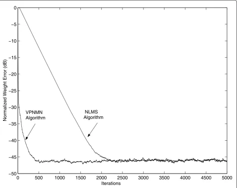
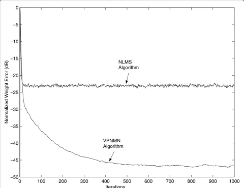
Figure 1 compares the fastest convergence characteris-tics of both the proposed algorithm and the NLMS algo-rithm. It can be seen from this figure that the proposed algorithm converges as fast as the NLMS algorithm but results in a lower weight mismatch. An improvement of 25 dB is obtained through the use of the proposed algo-rithm. Also, as shown in Figure 2, the proposed
algorithm outperforms the NLMS algorithm, for the lowest steady-state error reached by the later, thanks to its built-in gear-shifting mechanism which gives it an extra degree of freedom in this region.
The fast convergence obtained by the proposed algo-rithm can be justified by the fact that when far from the optimum solution, this algorithm exhibits faster conver-gence than the NLMS algorithm by automatically increasing the step size (gear-shifting property).
Figure 3 summarizes the performance of the proposed VPNMN algorithm in the three different noise environ-ments with an SNR of 20 dB when the input signal is white. As can be depicted from this figure that the best performance is obtained when the noise statistics are uniform while the worst performance is obtained when the noise statistics are laplacian.
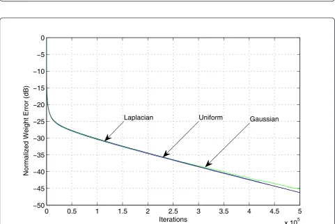
Similarly, Figure 4 depicts the results for the proposed VPNMN algorithm when the input signal is highly
0 500 1000 1500 2000 2500 3000 3500 4000 4500 5000
−50
−45
−40
−35
−30
−25
−20
−15
−10
−5 0
Iterations
Normalized Weight Error (dB)
NLMS Algorithm VPNMN
Algorithm
correlated and as can seen from this figure that almost equal performance is obtained by the VPNMN algo-rithm for the different noise statistics.
In order to verify the stability bound on step-size given in (48), we investigate it in a Gaussian environ-ment and an SNR of 20 dB. Here, we choose a misad-justment of five which results in the Cramer-Rao bound to be C≤ 0.05. Thus, choosing a tr(R) = 5, the upper bound given in (48) is found to be 0.95. It is observed from the various performed simulations that the NCLMF algorithm is stable whileµis less than 1.0 and thus, eventually validating the derived stability bound.
Finally, from the viewpoint of computational load the proposed algorithm requires an additional seven multi-plications and three additions when compared to the fixed mixed-norm algorithm defined by (4), and only eleven multiplications and six additions when compared to the NLMS algorithm. The small computational over
head of the proposed algorithm is therefore well worth the gain in the steady-state error reduction it brings about.
6.2 Results for the MSE learning curve
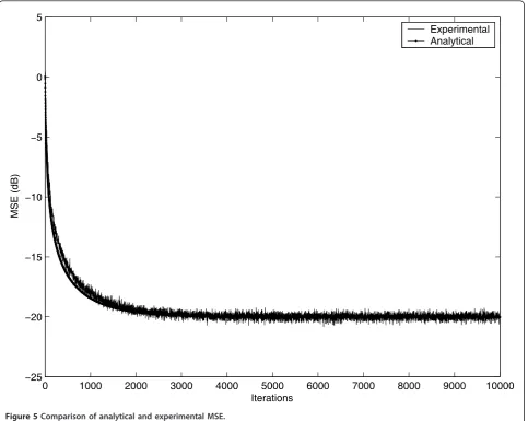
Figure 5 depicts the time evolution of the MSE obtained for both the theoretical analysis, the second entry of (44), and the simulations. Excellent agreement between theory and simulation results is obtained; hence, a con-sistency in performance is obtained by the proposed VPNMN algorithm.
6.3 Results for tracking
For tracking, the simulations are carried out for a sys-tem identification problem, where the unknown syssys-tem, having an FIR model, is given by [1.0119 - j0.7589, -0.3796 +j0.5059]T, while the system characteristics are time-varying according to the system model (54) and
0 100 200 300 400 500 600 700 800 900 1000
−50
−45
−40
−35
−30
−25
−20
−15
−10
−5 0
Iterations
Normalized Weight Error (dB)
VPNMN Algorithm
NLMS Algorithm
0 1 2 3 4 5 6 7 8 9 10 x 104
−60
−50
−40
−30
−20
−10 0
Iterations
Normalized Weight Error (dB)
Laplacian Gaussian Uniform
Figure 3Convergence behaviour of the VPNMN algorithm when the input signal is white.
0 0.5 1 1.5 2 2.5 3 3.5 4 4.5 5
x 105
−50
−45
−40
−35
−30
−25
−20
−15
−10
−5 0
Iterations
Normalized Weight Error (dB)
Laplacian Uniform Gaussian
(55). Results for the proposed algorithm are presented to validate the theoretical findings for different values ofΩ and different values of µ. The input signal xn to both the unknown system and the adaptive filter is a zero-mean white Gaussian sequence. The signal to noise ratio is set to be equal to 30 dB two values are consid-ered for tr{Qn}: a very small value of tr{Qn} = 10-7, and a very large one of tr{Qn} = 10-2.
Figure 6 depicts the comparison of the theory to the simulation results for three different values ofΩ, i.e.,Ω =0.001, 0.002, and 0.003. As can be seen from this fig-ure, close agreement between theory and simulation results are obtained. Furthermore, it is observed from this figure that degradation in performance is obtained by increasing the frequency offsetΩand unlike the sta-tionary case, the steady-state EMSE is not a monotoni-cally increasing function of the step-size µ, that is the steady-state EMSE is smaller at larger values of the step-sizeµ.
0 1000 2000 3000 4000 5000 6000 7000 8000 9000 10000
−25
−20
−15
−10
−5 0 5
Iterations
MSE (dB)
Experimental Analytical
Figure 5Comparison of analytical and experimental MSE.
0.1 0.2 0.3 0.4 0.5 0.6 0.7 0.8 0.9 1
−25
−20
−15
−10
−5 0 5
Steady state EMSE (dB)
=0.002
=0.003
=0.001
Figure 6 is obtained for the case when tr{Qn} = 10-7 which is represents a small value. Increasing this value to 10-2, the results depicted in Figure 7 for three larger values ofΩ, i.e., 0.01, 0.02, and 0.03, still show that the
previously stated observations are similar to those obtained for a smaller value of tr{Qn}.
Finally, the consistency in the performance of the steady-state EMSE of the proposed algorithm is observed in both cases (two different values of tr{Qn}) and different values ofΩ.
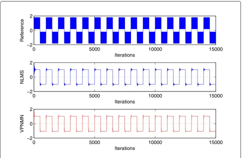
6.4 Noise cancelation using VPNMN algorithm
In this example, we study the performance of the VPNMN algorithm for the application of noise cancela-tion. A pure sinusoidal noise generated by the process (un = 0.8 sin (ωn + 0.5π)) with ω = 0.1 π is to be removed from a square wave generated by (sn = 2 × ((mod(n, 1000) <1000/2) - 0.5)) where mod (n, 1000) computes the modulus ofnover 1,000. Summingunand sn gives us the reference signal to the adaptive filter. The input to the adaptive filter is a sinusoidal signal generated by!xn=√2 sin(ωn)"with ω = 0.1 π. The resulting output error signalenwill, in time, converge to the desired signal which will be noiseless.
Figure 8 depicts the reference response and the pro-cessed results by the VPNMN algorithm and NLMS
0.1 0.2 0.3 0.4 0.5 0.6 0.7 0.8 0.9 1
−14
−12
−10
−8
−6
−4
−2 0
Steady state EMSE (dB)
=0.01
=0.02
=0.03
Figure 7Analytical (-) and experimental (Δ) steady-state EMSE forΩ=0.01,Ω=0.02, andΩ=0.03, and tr{Qk} = 10
-2 .
0 5000 10000 15000
−2 0 2
Iterations
Reference
0 5000 10000 15000
−2 0 2
Iterations
NLMS
0 5000 10000 15000
−2 0 2
Iterations
VPNMN
algorithm. It is clear that both algorithms are able to remove the noise component but VPNMN algorithm exhibits better noise cancelation capabilities as com-pared to the NLMS algorithm.
7 Conclusion
In this study, a normalized VPNMN algorithm is pro-posed where a combination of the LMS and the LMF algorithms is incorporated using the concept of variable step-size LMS adaptation. It is found that the proposed algorithm has the fast convergence property of the NLMS algorithm while resulting in a lower steady-state error, therefore eliminating the conflict between these two parameters, i.e., fast convergence and low steady-state error. Moreover, the consistency of the perfor-mance of the proposed algorithm has been confirmed by many simulation results which are reported here.
The analytical results of the tracking steady-state EMSE are derived for the proposed algorithm in the presence of both random and cyclic nonstationarities. The results, show that unlike in the stationary case, the steady-state EMSE is not a monotonically increasing function of the step-sizeµ, while the ability of the algo-rithm to track the variations in the environment degrades by increasing the frequency offsetΩ.
Finally, the VPNMN algorithm proved its usefulness in a noise cancelation scenario where it showed its superiority over the NLMS algorithm.
Acknowledgements
The author acknowledges the support of the Deanship of Scientific Research at King Fahd University of Petroleum & Minerals. This research work is funded by the King Fahd University of Petroleum & Minerals under Research Grants (FT090016) and (SB101024).
Competing interests
The author declares that they have no competing interests.
Received: 1 August 2011 Accepted: 5 March 2012 Published: 5 March 2012
References
1. B Widrow, JM McCool, MG Larimore, CR Johnson, Stationary and nonstationary learning characteristics of the LMS adaptive filter. Proc IEEE.
64(8), 1151–1162 (1976)
2. O Macchi,Adaptive Processing: The LMS Approach with Applications in TransmissionWiley, New York, (1995)
3. E Walach, B Widrow, The least mean fourth (LMF) adaptive algorithm and its family. IEEE Trans Inf Theory.30, 275–283 (1984). doi:10.1109/ TIT.1984.1056886
4. S Haykin,Adaptive Filter Theory, 3rd edn. (Prentice-Hall, Englewood Cliffs, 1996)
5. JI Nagumo, A Noda, A learning method for system identification. IEEE Trans Automat Control.12, 282–287 (1967)
6. A Zerguine, Convergence and steady-state analysis of the normalized least mean fourth algorithm. Digital Signal Process.17(1), 17–31 (2007). doi:10.1016/j.dsp.2006.01.005
7. A Zerguine, Convergence behavior of the normalized least mean fourth algorithm, inProc 34th Annual Asilomar Conf Signals, Syst Comput, 245–278 (2000)
8. MK Chan, CFN Cowan, Using a normalised LMF algorithm for channel equalisation with co-channel interference, inXI Euro Sig Process Conf Eusipco 2002.2, 49–51 (Sept. 2002)
9. O Tanrikulu, JA Chambers, Convergence and steady-state properties of the least mean mixed-norm (LMMN) adaptive filtering, inIEEE Proc.-Vis. Image Signal Process.143(3), 137–142 (June 1996)
10. A Zerguine, CFN Cowan, M Bettayeb, LMS-LMF adaptive scheme for echo cancellation. Electron Lett.32(19), 1776–1778 (1996). doi:10.1049/ el:19961202
11. TY Al-Naffouri, A Zerguine, M Bettayeb, Convergence properties of mixed-norm algorithms under general error criteria, inIEEE ISCAS‘99, 211–214 (1999)
12. M Tarrab, A Feuer, Convergence and performance analysis of the normalized LMS algorithm with uncorrelated gaussian data. IEEE Trans Inf Theory.34, 680–691 (1988). doi:10.1109/18.9768
13. AI Sulyman, A Zerguine, Convergence and steady-state analysis of a variable step-size NLMS algorithm. Signal Process.83(6), 1255–1273 (2003). doi:10.1016/S0165-1684(03)00044-6
14. A Zerguine, T Aboulnasr, Convergence analysis of the variable weight mixed-norm LMS-LMF adaptive algorithm, inProc 34th Annual Asilomar Conf Signals, Syst, Comput, 249–282 (2000)
15. T Aboulnasr, K Mayyas, A robust variable step-size LMS-type algorithm: analysis and simulations. IEEE Trans Signal Process.45(3), 631–639 (1997). doi:10.1109/78.558478
16. JE Mazo, On the independence theory of equalizer convergence. Bell Syst Tech J.58, 963–993 (1979)
17. SH Cho, SD Kim, KY Jean, Statistical convergence of the adaptive least mean fourth algorithm, inProceedings of the ICSP’96, 610–613 (1996) 18. PI Hubscher, JCM Bermudez, An improved statistical analysis of the least
mean fourth (LMF) adaptive algorithm. IEEE Trans Signal Process.51(3), 664–671 (2003). doi:10.1109/TSP.2002.808126
19. JG Proakis,Digital Communications, 4th edn. (McGraw-Hill, Singapore, 2001) 20. M Rupp, AH Sayed, A time-domain feedback analysis of filtered-error
adaptive gradient algorithms. IEEE Trans Signal Process.44, 1428–1439 (1996). doi:10.1109/78.506609
21. AH Sayed,Adaptive FiltersWiley, NJ, (2008)
22. NJ Bershad, M Bonnet, Saturation effects in LMS adaptive echo cancellation for binary data. IEEE Trans Acoust Speech Signal Process.38(10), 1687–1696 (1990). doi:10.1109/29.60100
23. A Papoulis,Probability, Random Variables, and Stochastic Processes (McGraw-Hill, New York, 1991)
24. SC Douglas, TH-Y Meng, Stochastic gradient adaptation under general error criteria. IEEE Trans Signal Process.42(6), 1352–1365 (1994). doi:10.1109/ 78.286952
25. NR Yousef, AH Sayed, A unified approach to the steady-state and tracking analysis of adaptive filters. IEEE Trans Signal Process.49, 314–324 (2001). doi:10.1109/78.902113
26. TS Rappaport,Wireless Communications(Prentice-Hall, Upper Saddle River, 1996)
27. M Rupp, LMS tracking behavior under periodically changing systems, in EUSIPCO-1998, Island of Rhodes, Greece, 1253–1256 (Sept 1998) 28. M Moinuddin, A Zerguine, Tracking analysis of the NLMS algorithm in the
presence of both random and cyclic nonstationarities. IEEE Signal Process Lett.10(9), 256–258 (2003)
29. M Moinuddin, A Zerguine, AUH Sheikh, Tracking analysis of the NLMF algorithm in the presence of both random and cyclic nonstationarities, in ISSPA 2005, Sydney, Australia, 755–758 (Aug 2005)
doi:10.1186/1687-6180-2012-55