Guide to NumPy
Travis E. Oliphant, PhD
Dec 7, 2006
Contents
I
NumPy from Python
12
1 Origins of NumPy 13
2 Object Essentials 18
2.1 Data-Type Descriptors . . . 20
2.2 Basic indexing (slicing). . . 23
2.3 Memory Layout ofndarray . . . 26
2.3.1 Contiguous Memory Layout . . . 26
2.3.2 Non-contiguous memory layout . . . 28
2.4 Universal Functions for arrays. . . 30
2.5 Summary of new features . . . 32
2.6 Summary of differences with Numeric . . . 34
2.6.1 First-step changes . . . 34
2.6.2 Second-step changes . . . 37
2.6.3 Updating code that uses Numeric using alter codeN . . . 38
2.6.4 Changes to think about . . . 39
2.7 Summary of differences with Numarray . . . 40
2.7.1 First-step changes . . . 41
2.7.1.1 Import changes. . . 41
2.7.1.2 Attribute and method changes . . . 42
2.7.2 Second-step changes . . . 43
2.7.3 Additional Extension modules. . . 43
3 The Array Object 45 3.1 ndarrayAttributes . . . 45
3.1.1 Memory Layout attributes. . . 46
3.1.3 Other attributes . . . 51
3.1.4 Array Interface attributes . . . 52
3.2 ndarrayMethods . . . 55
3.2.1 Array conversion . . . 55
3.2.2 Array shape manipulation . . . 60
3.2.3 Array item selection and manipulation . . . 62
3.2.4 Array calculation . . . 66
3.3 Array Special Methods . . . 72
3.3.1 Methods for standard library functions. . . 72
3.3.2 Basic customization . . . 73
3.3.3 Container customization . . . 75
3.3.4 Arithmetic customization . . . 76
3.3.4.1 Binary . . . 76
3.3.4.2 In-place . . . 78
3.3.4.3 Unary operations . . . 79
3.4 Array indexing . . . 80
3.4.1 Basic Slicing . . . 80
3.4.2 Advanced selection . . . 82
3.4.2.1 Integer . . . 82
3.4.2.2 Boolean . . . 84
3.4.3 Flat Iterator indexing . . . 85
4 Basic Routines 86 4.1 Creating arrays . . . 86
4.2 Operations on two or more arrays. . . 91
4.3 Printing arrays . . . 94
4.4 Functions redundant with methods . . . 95
4.5 Dealing with data types . . . 96
5 Additional Convenience Routines 98 5.1 Shape functions . . . 98
5.2 Basic functions . . . 102
5.3 Polynomial functions . . . 110
5.4 Set Operations . . . 113
5.5 Array construction using index tricks. . . 114
5.6 Other indexing devices . . . 117
5.8 More data type functions . . . 120
5.9 Functions that behave like ufuncs . . . 123
5.10 Miscellaneous Functions . . . 123
5.11 Utility functions . . . 126
6 Scalar objects 128 6.1 Attributes of array scalars . . . 129
6.2 Methods of array scalars . . . 131
6.3 Defining New Types . . . 132
7 Data-type (dtype) Objects 133 7.1 Attributes . . . 134
7.2 Construction . . . 136
7.3 Methods . . . 139
8 Standard Classes 141 8.1 Special attributes and methods recognized by NumPy . . . 142
8.2 Matrix Objects . . . 143
8.3 Memory-mapped-file arrays . . . 145
8.4 Character arrays (numpy.char) . . . 146
8.5 Record Arrays (numpy.rec) . . . 147
8.6 Masked Arrays (numpy.ma) . . . 151
8.7 Standard container class . . . 152
8.8 Array Iterators . . . 152
8.8.1 Default iteration . . . 153
8.8.2 Flat iteration . . . 153
8.8.3 N-dimensional enumeration . . . 154
8.8.4 Iterator for broadcasting. . . 154
9 Universal Functions 156 9.1 Description . . . 156
9.1.1 Broadcasting . . . 157
9.1.2 Output type determination . . . 157
9.1.3 Use of internal buffers . . . 158
9.1.4 Error handling . . . 158
9.1.5 Optional keyword arguments . . . 159
9.2 Attributes . . . 160
9.4 Methods . . . 162
9.4.1 Reduce . . . 164
9.4.2 Accumulate . . . 164
9.4.3 Reduceat . . . 165
9.4.4 Outer . . . 166
9.5 Available ufuncs . . . 167
9.5.1 Math operations . . . 167
9.5.2 Trigonometric functions . . . 170
9.5.3 Bit-twiddling functions. . . 171
9.5.4 Comparison functions . . . 172
9.5.5 Floating functions . . . 174
10 Basic Modules 177 10.1 Linear Algebra (linalg) . . . 177
10.2 Discrete Fourier Transforms (fft) . . . 180
10.3 Random Numbers (random) . . . 184
10.3.1 Discrete Distributions . . . 185
10.3.2 Continuous Distributions . . . 187
10.3.3 Miscellaneous utilities . . . 194
10.4 Matrix-specific functions (matlib) . . . 194
10.5 Ctypes utiltity functions (ctypeslib) . . . 194
11 Testing and Packaging 196 11.1 Testing . . . 196
11.2 NumPy Distutils . . . 199
11.2.1 misc util. . . 199
11.2.2 Other modules . . . 206
11.3 Conversion of .src files . . . 208
11.3.1 Fortran files . . . 208
11.3.1.1 Named repeat rule . . . 208
11.3.1.2 Short repeat rule. . . 208
11.3.1.3 Pre-defined names . . . 209
11.3.2 Other files. . . 209
II
C-API
211
12.1 New Python Types Defined . . . 213
12.1.1 PyArray Type . . . 214
12.1.2 PyArrayDescr Type . . . 215
12.1.3 PyUFunc Type . . . 223
12.1.4 PyArrayIter Type . . . 226
12.1.5 PyArrayMultiIter Type . . . 227
12.1.6 PyArrayFlags Type . . . 228
12.1.7 ScalarArrayTypes . . . 228
12.2 Other C-Structures . . . 229
12.2.1 PyArray Dims . . . 229
12.2.2 PyArray Chunk. . . 230
12.2.3 PyArrayInterface . . . 230
12.2.4 Internally used structures . . . 232
12.2.4.1 PyUFuncLoopObject . . . 232
12.2.4.2 PyUFuncReduceObject . . . 232
12.2.4.3 PyUFunc Loop1d . . . 232
12.2.4.4 PyArrayMapIter Type . . . 232
13 Complete API 233 13.1 Configuration defines . . . 233
13.1.1 Guaranteed to be defined . . . 233
13.1.2 Possible defines . . . 234
13.2 Array Data Types . . . 235
13.2.1 Enumerated Types . . . 235
13.2.2 Defines . . . 236
13.2.2.1 Max and min values for integers . . . 236
13.2.2.2 Number of bits in data types . . . 236
13.2.2.3 Bit-width references to enumerated typenums. . . . 237
13.2.2.4 Integer that can hold a pointer . . . 237
13.2.3 C-type names . . . 237
13.2.3.1 Boolean . . . 237
13.2.3.2 (Un)Signed Integer . . . 237
13.2.3.3 (Complex) Floating point . . . 238
13.2.3.4 Bit-width names . . . 238
13.2.4 Printf Formatting . . . 238
13.3 Array API . . . 239
13.3.1.1 Data access. . . 240
13.3.2 Creating arrays . . . 241
13.3.2.1 From scratch . . . 241
13.3.2.2 From other objects. . . 244
13.3.3 Dealing with types . . . 249
13.3.3.1 General check of Python Type . . . 249
13.3.3.2 Data-type checking . . . 251
13.3.3.3 Converting data types . . . 254
13.3.3.4 New data types . . . 256
13.3.3.5 Special functions for PyArray OBJECT . . . 257
13.3.4 Array flags . . . 258
13.3.4.1 Basic Array Flags . . . 258
13.3.4.2 Combinations of array flags. . . 259
13.3.4.3 Flag-like constants . . . 259
13.3.4.4 Flag checking. . . 260
13.3.5 Array method alternative API . . . 261
13.3.5.1 Conversion . . . 261
13.3.5.2 Shape Manipulation . . . 263
13.3.5.3 Item selection and manipulation . . . 265
13.3.5.4 Calculation . . . 268
13.3.6 Functions . . . 270
13.3.6.1 Array Functions . . . 270
13.3.6.2 Other functions . . . 272
13.3.7 Array Iterators . . . 273
13.3.8 Broadcasting (multi-iterators). . . 274
13.3.9 Array Scalars . . . 276
13.3.10 Data-type descriptors . . . 278
13.3.11 Conversion Utilities . . . 280
13.3.11.1 For use withPyArg ParseTuple . . . 280
13.3.11.2 Other conversions . . . 282
13.3.12 Miscellaneous . . . 283
13.3.12.1 Importing the API. . . 283
13.3.12.2 Internal Flexibility. . . 284
13.3.12.3 Memory management . . . 285
13.3.12.4 Threading support. . . 285
13.3.12.5 Priority . . . 287
13.3.12.7 Other constants . . . 287
13.3.12.8 Miscellaneous Macros . . . 288
13.3.12.9 Enumerated Types. . . 289
13.4 UFunc API . . . 289
13.4.1 Constants . . . 289
13.4.2 Macros . . . 290
13.4.3 Functions . . . 290
13.4.4 Generic functions . . . 293
13.5 Importing the API . . . 295
14 How to extend NumPy 297 14.1 Writing an extension module . . . 297
14.2 Required subroutine . . . 298
14.3 Defining functions . . . 299
14.3.1 Functions without keyword arguments . . . 300
14.3.2 Functions with keyword arguments . . . 301
14.3.3 Reference counting . . . 302
14.4 Dealing with array objects . . . 303
14.4.1 Converting an arbitrary sequence object . . . 304
14.4.2 Creating a brand-new ndarray . . . 307
14.4.3 Getting at ndarray memory and accessing elements of the ndarray . . . 308
14.5 Example . . . 309
15 Beyond the Basics 311 15.1 Iterating over elements in the array. . . 311
15.1.1 Basic Iteration . . . 311
15.1.2 Iterating over all but one axis . . . 313
15.1.3 Iterating over multiple arrays . . . 313
15.1.4 Broadcasting over multiple arrays . . . 314
15.2 Creating a new universal function. . . 315
15.3 User-defined data-types . . . 318
15.3.1 Adding the new data-type . . . 319
15.3.2 Registering a casting function . . . 319
15.3.3 Registering coercion rules . . . 320
15.3.4 Registering a ufunc loop . . . 321
15.4.1 Creating sub-types . . . 322
15.4.2 Specific features of ndarray sub-typing . . . 323
15.4.2.1 The array finalize method . . . 323
15.4.2.2 The array priority attribute . . . 324
15.4.2.3 The array wrap method . . . 324
16 Using Python as glue 325 16.1 Calling other compiled libraries from Python . . . 326
16.2 Hand-generated wrappers . . . 327
16.3 f2py . . . 327
16.3.1 Creating source for a basic extension module . . . 328
16.3.2 Creating a compiled extension module . . . 328
16.3.3 Improving the basic interface . . . 329
16.3.4 Inserting directives in Fortran source. . . 330
16.3.5 A filtering example . . . 331
16.3.6 Calling f2py from Python . . . 332
16.3.7 Automatic extension module generation . . . 333
16.3.8 Conclusion . . . 333
16.4 weave . . . 334
16.4.1 Speed up code involving arrays (also see scipy.numexpr) . . . 334
16.4.2 Inline C-code . . . 335
16.4.3 Simplify creation of an extension module . . . 337
16.4.4 Conclusion . . . 338
16.5 Pyrex . . . 338
16.5.1 Pyrex-add. . . 340
16.5.2 Pyrex-filter . . . 341
16.5.3 Conclusion . . . 342
16.6 ctypes . . . 343
16.6.1 Having a shared library . . . 344
16.6.2 Loading the shared library . . . 345
16.6.3 Converting arguments . . . 346
16.6.4 Calling the function . . . 347
16.6.5 Complete example . . . 348
16.6.6 Conclusion . . . 352
16.7 Additional tools you may find useful . . . 353
16.7.1 SWIG . . . 353
16.7.3 Boost Python. . . 354
16.7.4 Instant . . . 355
16.7.5 PyInline . . . 356
16.7.6 PyFort. . . 356
17 Code Explanations 357 17.1 Memory model . . . 357
17.2 Data-type encapsulation . . . 358
17.3 N-D Iterators . . . 359
17.4 Broadcasting . . . 359
17.5 Array Scalars . . . 360
17.6 Advanced (“Fancy”) Indexing . . . 361
17.6.1 Fancy-indexing check. . . 361
17.6.2 Fancy-indexing implementation . . . 362
17.6.2.1 Creating the mapping object . . . 362
17.6.2.2 Binding the mapping object . . . 362
17.6.2.3 Getting (or Setting) . . . 363
17.7 Universal Functions . . . 363
17.7.1 Setup . . . 364
17.7.2 Function call . . . 365
17.7.2.1 One Loop. . . 366
17.7.2.2 Strided Loop . . . 366
17.7.2.3 Buffered Loop . . . 366
17.7.3 Final output manipulation. . . 367
17.7.4 Methods. . . 367
17.7.4.1 Setup . . . 367
17.7.4.2 Reduce . . . 368
17.7.4.3 Accumulate. . . 369
List of Tables
2.1 Built-in array-scalar types corresponding to data-types for an ndar-ray. The bold-face types correspond to standard Python types. The object type is special because arrays with dtype=’O’ do not return an array scalar on item access but instead return the actual object referenced in the array.. . . 22
3.1 Attributes of thendarray. . . 47
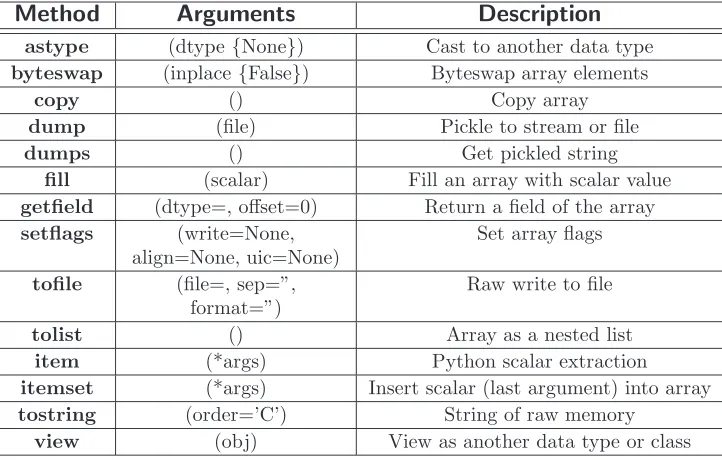
3.2 Array conversion methods . . . 59
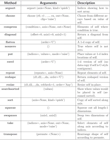
3.3 Array item selection and shape manipulation methods. If axis is an argument, then the calculation is performed along that axis. An axis value of None means the array is flattened before calculation proceeds. 67
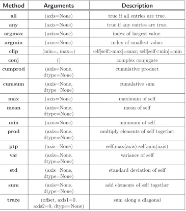
3.4 Array object calculation methods. If axis is an argument, then the calculation is performed along that axis. An axis value of None means the array is flattened before calculation proceeds. All of these meth-ods can take an optional out= argument which can specify the output array to write the results into. . . 71
6.1 Array scalar types that inherit from basic Python types. The intc array data type might also inherit from the IntType if it has the same number of bits as the int array data type on your platform.. . . 129
9.1 Universal function (ufunc) attributes. . . 161
Part I
Chapter 1
Origins of NumPy
A complex system that works is invariably found to have evolved from a simple system that worked
—John Gall
Copy from one, it’s plagiarism; copy from two, it’s research.
—Wilson Mizner
NumPy builds on (and is a successor to) the successful Numeric array object. Its goal is to create the corner-stone for a useful environment for scientific com-puting. In order to better understand the people surrounding NumPy and (its library-package) SciPy, I will explain a little about how SciPy and (current) NumPy originated. In 1998, as a graduate student studying biomedical imaging at the Mayo Clinic in Rochester, MN, I came across Python and its numerical extension (Numeric) while I was looking for ways to analyze large data sets for Magnetic Resonance Imaging and Ultrasound using a high-level language. I quickly fell in love with Python programming which is a remarkable statement to make about a programming language. If I had not seen others with the same view, I might have seriously doubted my sanity. I became rather involved in the Numeric Python com-munity, adding the C-API chapter to the Numeric documentation (for which Paul Dubois graciously made me a co-author).
when a task I needed to perform was not available in the core language, or in the Numeric extension, I looked around and found C or Fortran code that performed the needed task, wrapped it into Python (either by hand or using SWIG), and used the new functionality in my programs.
Along the way, I learned a great deal about the underlying structure of Numeric and grew to admire it’s simple but elegant structures that grew out of the mechanism by which Python allows itself to be extended.
NOTE
Numeric was originally written in 1995 largely by Jim Hugunin while he was a graduate student at MIT. He received help from many people including Jim Fulton, David Ascher, Paul Dubois, and Konrad Hinsen. These individuals and many others added comments, criticisms, and code which helped the Numeric exten-sion reach stability. Jim Hugunin did not stay long as an active member of the community — moving on to write Jython and, later, Iron Python.
By operating in this need-it-make-it fashion I ended up with a substantial li-brary of extension modules that helped Python + Numeric become easier to use in a scientific setting. These early modules included raw input-output functions, a special function library, an integration library, an ordinary differential equation solver, some least-squares optimizers, and sparse matrix solvers. While I was doing this laborious work, Pearu Peterson noticed that a lot of the routines I was wrap-ping were written in Fortran and there was no simplified wrapwrap-ping mechanism for Fortran subroutines (like SWIG for C). He began the task of writing f2py which made it possible to easily wrap Fortran programs into Python. I helped him a little bit, mostly with testing and contributing early function-call-back code, but he put forth the brunt of the work. His result was simply amazing to me. I’ve always been impressed with f2py, especially because I knew how much effort writing and main-taining extension modules could be. Anybody serious about scientific computing with Python will appreciate that f2py is distributed along with NumPy.
code to SciPy including Ed Schofield, Robert Cimrman, David M. Cooke, Charles (Chuck) Harris, Prabhu Ramachandran, Gary Strangman, Jean-Sebastien Roy, and Fernando Perez. Others such as Travis Vaught, David Morrill, Jeff Whitaker, and Louis Luangkesorn have contributed testing and build support.
At the start of 2005, SciPy was at release 0.3 and relatively stable for an early version number. Part of the reason it was difficult to stabilize SciPy was that the array object upon which SciPy builds was undergoing a bit of an upheaval. At about the same time as SciPy was being built, some Numeric users were hitting up against the limited capabilities of Numeric. In particular, the ability to deal with memory mapped files (and associated alignment and swapping issues), record arrays, and altered error checking modes were important but limited or non-existent in Numeric. As a result, numarray was created by Perry Greenfield, Todd Miller, and Rick White at the Space Science Telescope Institute as a replacement for Numeric. Numarray used a very different implementation scheme as a mix of Python classes and C code (which led to slow downs in certain common uses). While improving some capabilities, it was slow to pick up on the more advanced features of Numeric’s universal functions (ufuncs) — never re-creating the C-API that SciPy depended on. This made it difficult for SciPy to “convert” to numarray.
Many newcomers to scientific computing with Python were told that numarray was the future and started developing for it. Very useful tools were developed that could not be used with Numeric (because of numarray’s change in C-API), and therefore could not be used easily in SciPy. This state of affairs was very discouraging for me personally as it left the community fragmented. Some developed for numarray, others developed as part of SciPy. A few people even rejected adopting Python for scientific computing entirely because of the split. In addition, I estimate that quite a few Python users simply stayed away from both SciPy and numarray, leaving the community smaller than it could have been given the number of people that use Python for science and engineering purposes.
It should be recognized that the split was not intentional, but simply an out-growth of the different and exacting demands of scientific computing users. My describing these events should not be construed as assigning blame to anyone. I very much admire and appreciate everyone I’ve met who is involved with scientific computing and Python. Using a stretched biological metaphor, it is only through the process of dividing and merging that better results are born. I think this concept applies to NumPy.
to see what could be done to add the missing features to make SciPy work with it as a core array object. After a couple of days of studying numarray, I was not enthusiastic about this approach. My familiarity with the Numeric code base no doubt biased my opinion, but it seemed to me that the features of Numarray could be added back to Numeric with a few fundamental changes to the core object. This would make the transition of SciPy to a more enhanced array object much easier in my mind.
Therefore, I began to construct this hybrid array object complete with an en-hanced set of universal (broadcasting) functions that could deal with it. Along the way, quite a few new features and significant enhancements were added to the array object and its surrounding infrastructure. This book describes the result of that year-and-a-half-long effort which culminated with the release of NumPy 0.9.2 in early 2006 and NumPy 1.0 in late 2006. I first named the new package, SciPy Core, and used the scipy namespace. However, after a few months of testing under that name, it became clear that a separate namespace was needed for the new package. As a result, a rapid search for a new name resulted in actually coming back to the NumPy name which was the unofficial name of Numerical Python but never the actual namespace. Because the new package builds on the code-base of and is a successor to Numeric, I think the NumPy name is fitting and hopefully not too confusing to new users.
This book only briefly outlines some of the infrastructure that surrounds the basic objects in NumPy to provide the additional functionality contained in the older Numeric package (i.e. LinearAlgebra, RandomArray, FFT). This infrastructure in NumPy includes basic linear algebra routines, Fourier transform capabilities, and random number generators. In addition, the f2py module is described in its own documentation, and so is only briefly mentioned in the second part of the book. There are also extensions to the standard Python distutils and testing frameworks included with NumPy that are useful in constructing your own packages built on top of NumPy. The central purpose of this book, however, is to describe and document the basic NumPy system that is available under the numpy namespace.
NOTE
The following table gives a brief outline of the sub-packages contained in numpy package.
Sub-Package Purpose Comments
core basic objects all names exported to numpy
lib additional utilities all names exported to numpy linalg basic linear algebra old LinearAlgebra from Numeric
fft discrete Fourier transforms old FFT from Numeric random random number generators old RandomArray from Numeric distutils enhanced build and distribution improvements built on standard distutils
Chapter 2
Object Essentials
Our programs last longer if we manage to build simple abstractions for ourselves...
—Ron Jeffries
I will tell you the truth as soon as I figure it out.
—Wayne Birmingham
NumPy provides two fundamental objects: an N-dimensional array object (ndarray) and a universal function object (ufunc). In addition, there are other objects that build on top of these which you may find useful in your work, and these will be discussed later. The current chapter will provide background information on just thendarrayand theufuncthat will be important for understanding the attributes and methods to be discussed later.
of memory in the array is interpreted in exactly the same way1.
i
TIP
All arrays in NumPy are indexed starting at 0 and ending at M-1 following the Python convention.
For example, consider the following piece of code:
>>> a = array([[1,2,3],[4,5,6]]) >>> a.shape
(2, 3) >>> a.dtype dtype(’int32’)
NOTE
for all code in this book it is assumed that you have first entered
from numpy import *. In addition, any previously defined ar-rays are still defined for subsequent examples.
This code defines an array of size 2×3 composed of 4-byte (little-endian) integer elements (on my 32-bit platform). We can index into this two-dimensional array using two integers: the first integer running from 0 to 1 inclusive and the second from 0 to 2 inclusive. For example, index (1,1) selects the element with value 5:
>>> a[1,1] 5
All code shown in the shaded-boxes in this book has been (automatically) exe-cuted on a particular version of NumPy. The output of the code shown below shows which version of NumPy was used to create all of the output in your copy of this book.
>>> import numpy; print numpy. version 1.0.2.dev3478
1
header
...
ndarray
scalar array
head
data−type
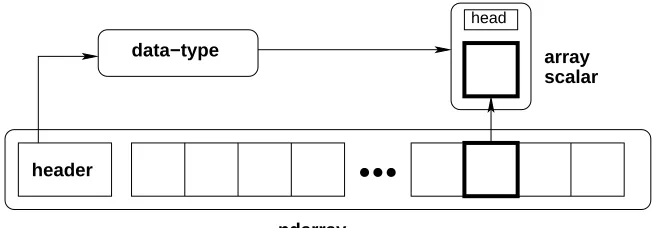
Figure 2.1: Conceptual diagram showing the relationship between the three fun-damental objects used to describe the data in an array: 1) the ndarray itself, 2) the data-type object that describes the layout of a single fixed-size element of the array, 3) the array-scalar Python object that is returned when a single element of the array is accessed.
2.1
Data-Type Descriptors
In NumPy, an ndarray is anN-dimensional array of items where each item takes up a fixed number of bytes. Typically, this fixed number of bytes represents a number (e.g. integer or floating-point). However, this fixed number of bytes could also represent an arbitrary record made up of any collection of other data types. NumPy achieves this flexibility through the use of a data-type (dtype) object. Every array has an associated dtype object which describes the layout of the array data. Every dtype object, in turn, has an associated Python type-object that determines exactly what type of Python object is returned when an element of the array is accessed. The dtype objects are flexible enough to contain references to arrays of other dtype objects and, therefore, can be used to define nested records. This advanced functionality will be described in better detail later as it is mainly useful for the recarray (record array) subclass that will also be defined later. However, all ndarrays can enjoy the flexibility provided by the dtype objects. Figure2.1provides a conceptual diagram showing the relationship between the ndarray, its associated data-type object, and an array-scalar that is returned when a single-element of the array is accessed. Note that the data-type points to the type-object of the array scalar. An array scalar is returned using the type-object and a particular element of the ndarray.
and complex data types. Associated with each data-type is a Python type object whose instances are array scalars. This type-object can be obtained using thetype
attribute of the dtype object. Python typically defines only one data-type of a particular data class (one integer type, one floating-point type, etc.). This can be convenient for some applications that don’t need to be concerned with all the ways data can be represented in a computer. For scientific applications, however, this is not always true. As a result, in NumPy, their are 21 different fundamental Python data-type-descriptor objects built-in. These descriptors are mostly based on the types available in the C language that CPython is written in. However, there are a few types that are extremely flexible, such asstr,unicode , andvoid.
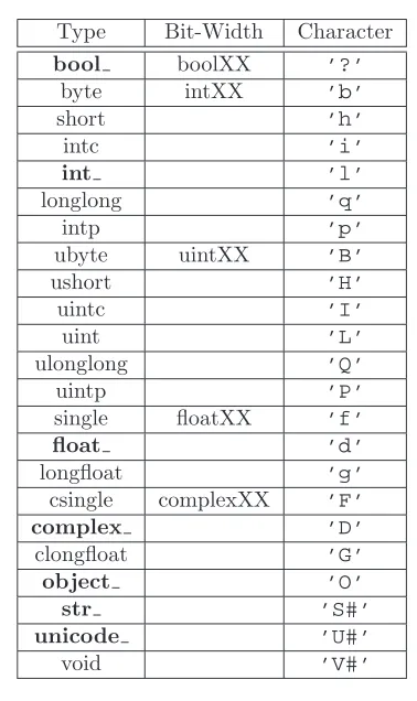
The fundamental data-types are shown in Table 2.1. Along with their (mostly) C-derived names, the integer, float, and complex data-types are also available using a bit-width convention so that an array of the right size can always be ensured (e.g. int8, float64, complex128). The C-like names are also accessible using a character code which is also shown in the table (use of the character codes, however, is discouraged). Names for the data types that would clash with standard Python object names are followed by a trailing underscore, ’ ’. These data types are so named because they use the same underlying precision as the corresponding Python data types. Most scientific users should be able to use the array-enhanced scalar objects in place of the Python objects. The array-enhanced scalars inherit from the Python objects they can replace and should act like them under all circumstances (except for how errors are handled in math computations).
i
TIP
The array types bool, int, complex, float, object , uni-code , and str are enhanced-scalars. They are very similar to the standard Python types (without the trailing underscore) and inherit from them (except for bool and object ). They can be used in place of the standard Python types whenever desired. Whenever a data type is required, as an argument, the standard Python types are recognized as well.
Table 2.1: Built-in array-scalar types corresponding to data-types for an ndarray. The bold-face types correspond to standard Python types. The object type is special because arrays with dtype=’O’ do not return an array scalar on item access but instead return the actual object referenced in the array.
Type Bit-Width Character
bool boolXX ’?’
byte intXX ’b’
short ’h’
intc ’i’
int ’l’
longlong ’q’
intp ’p’
ubyte uintXX ’B’
ushort ’H’
uintc ’I’
uint ’L’
ulonglong ’Q’
uintp ’P’
single floatXX ’f’
float ’d’
longfloat ’g’
csingle complexXX ’F’
complex ’D’
clongfloat ’G’
object ’O’
str ’S#’
unicode ’U#’
void ’V#’
basicndarray.
NOTE
WARNING
Numeric Compatibility: If you used old typecode characters in your Numeric code (which was never recommended), you will need to change some of them to the new characters. In particular, the needed changes are ’c->’S1’, ’b’->’B’, ’1’->’b’, ’s’->’h’, ’w’->’H’, and ’u’->’I’. These changes make the typecharacter conven-tion more consistent with other Python modules such as the struct module.
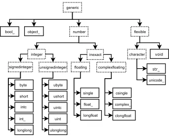
The fundamental data-types are arranged into a hierarchy of Python type-objects shown in Figure 2.2. Each of the leaves on this hierarchy correspond to actual data-types that arrays can have (in other words, there is a built in dtype ob-ject associated with each of these new types). They also correspond to new Python objects that can be created. These new objects are “scalar” types corresponding to each fundamental data-type. Their purpose is to smooth out the rough edges that result when mixing scalar and array operations. These scalar objects will be discussed in more detail in Chapter 6. The other types in the hierarchy define particular categories of types. These categories can be useful for testing whether or not the object returned by self.dtype.typeis of a particular class (using
issubclass).
2.2
Basic indexing (slicing)
Indexing is a powerful tool in Python and NumPy takes full advantage of this power. In fact, some of capabilities of Python’s indexing were first established by the needs of Numeric users.2 Indexing is also sometimes called slicing in Python, and slicing
for anndarrayworks very similarly as it does for other Python sequences. There are three big differences: 1) slicing can be done over multiple dimensions, 2) exactly one ellipsis object can be used to indicate several dimensions at once, 3) slicing cannot be used to expand the size of an array (unlike lists).
A few examples should make slicing more clear. Suppose A is a 10×20 array, thenA[3] is the same asA[3,:] and represents the 4th length-20 “row” of the array. On the other hand,A[:,3] represents the 4th length-10 “column” of the array. Every
2
third element of the 4th column can be selected asA[:: 3,3]. Ellipses can be used to replace zero or more “:” terms. In other words, an Ellipsis object expands to zero or more full slice objects (“:”) so that the total number of dimensions in the slicing tuple matches the number of dimensions in the array. Thus, ifAis 10×20×30×40, thenA[3 :, ...,4] is equivalent toA[3 :,:,:,4] whileA[...,3] is equivalent toA[:,:,:,3].
The following code illustrates some of these concepts:
>>> a = arange(60).reshape(3,4,5); print a [[[ 0 1 2 3 4]
[ 5 6 7 8 9] [10 11 12 13 14] [15 16 17 18 19]] [[20 21 22 23 24] [25 26 27 28 29] [30 31 32 33 34] [35 36 37 38 39]] [[40 41 42 43 44] [45 46 47 48 49] [50 51 52 53 54] [55 56 57 58 59]]]
>>> print a[...,3] [[ 3 8 13 18] [23 28 33 38] [43 48 53 58]]
>>> print a[1,...,3] [23 28 33 38]
>>> print a[:,:,2] [[ 2 7 12 17] [22 27 32 37] [42 47 52 57]]
>>> print a[0,::2,::2] [[ 0 2 4]
2.3
Memory Layout of
ndarray
On a fundamental level, anN-dimensional array object is just a one-dimensional se-quence of memory with fancy indexing code that maps anN-dimensional index into a one-dimensional index. The one-dimensional index is necessary on some level be-cause that is how memory is addressed in a computer. The fancy indexing, however, can be very helpful for translating our ideas into computer code. This is because many concepts we wish to model on a computer have a natural representation as an N-dimensional array. While this is especially true in science and engineering, it is also applicable to many other arenas which can be appreciated by considering the popularity of the spreadsheet as well as “image processing” applications.
WARNING
Some high-level languages give pre-eminence to a particular use of 2-dimensional arrays as Matrices. In NumPy, however, the core object is the more generalN-dimensional array. NumPy defines a matrix object as a sub-class of the N-dimensional array.
In order to more fully understand the array object along with its attributes and methods it is important to learn more about how an N-dimensional array is represented in the computer’s memory. A complete understanding of this layout is only essential for optimizing algorithms operating on general purpose arrays. But, even for the casual user, a general understanding of memory layout will help to explain the use of certain array attributes that may otherwise be mysterious.
2.3.1
Contiguous Memory Layout
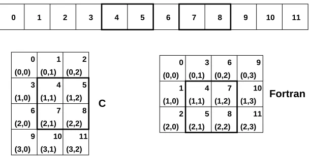
There is a fundamental ambiguity in how the mapping to a one-dimensional index can take place which is illustrated for a 2-dimensional array in Figure2.3. In that figure, each block represents a chunk of memory that is needed for representing the underlying array element. For example, each block could represent the 8 bytes needed to represent a double-precision floating point number.
11 10 9 8 7 6 5 4 3 2 1 0 C 11 10 9 8 7 6 5 4 3 2 1 0 (0,0) (0,2)
(1,0) (1,1) (1,2)
(2,2) (3,2) (0,1) (2,0) (3,0) (2,1) (3,1) Fortran 11 10 9 8 7 6 5 4 3 2 1 0
(0,0) (0,1) (0,2)
(1,0) (1,1) (1,2)
(2,0) (2,1) (2,2) (1,3)
(2,3) (0,3)
Figure 2.3: Options for memory layout of a 2-dimensional array.
In the C-style of N-dimensional indexing shown on the left of Figure 2.3 the last N-dimensional index “varies the fastest.” In other words, to move through computer memory sequentially, the last index is incremented first, followed by the second-to-last index and so forth. Some of the algorithms in NumPy that deal with N-dimensional arrays work best with this kind of data.
In the Fortran-style ofN-dimensional indexing shown on the right of Figure2.3, the firstN-dimensional index “varies the fastest.” Thus, to move through computer memory sequentially, the first index is incremented first until it reaches the limit in that dimension, then the second index is incremented and the first index is reset to zero. While NumPy can be compiled without the use of a Fortran compiler, several modules of SciPy (available separately) rely on underlying algorithms written in Fortran. Algorithms that work onN-dimensional arrays that are written in Fortran typically expect Fortran-style arrays.
The two-styles of memory layout for arrays are connected through the transpose operation. Thus, ifAis a (contiguous) C-style array, then the same block of mem-ory can be used to representAT as a (contiguous) Fortran-style array. This kind
2.3.2
Non-contiguous memory layout
Both of the examples presented above are single-segment arrays where the entire array is visited by sequentially marching through memory one element at a time. When an algorithm in C or Fortran expects an N-dimensional array, this single segment (of a certain fundamental type) is usually what is expected along with the shapeN-tuple. With a single-segment of memory representing the array, the one-dimensional index into computer memory can always be computed from the N-dimensional index. This concept is explored further in the following paragraphs. Letnibe the value of the ithindex into an array whose shape is represented by
theN integersdi (i= 0. . . N−1).Then, the one-dimensional index into a C-style
contiguous array is
nC=
N−1 X
i=0 ni
N−1 Y
j=i+1 dj
while the one-dimensional index into a Fortran-style contiguous array is
nF = N−1
X
i=0 ni
i−1 Y
j=0 dj.
In these formulas we are assuming that
m
Y
j=k
dj=dkdk+1· · ·dm−1dm
so that ifm < k,the product is 1.While perfectly general, these formulas may be a bit confusing at first glimpse. Let’s see how they expand out for determining the one-dimensional index corresponding to the element (1,3,2) of a 4×5×6 array. If the array is stored as Fortran contiguous, then
nF = n0·(1) +n1·(4) +n2·(4·5) = 1 + 3·4 + 2·20 = 53.
On the other hand, if the array is stored as C contiguous, then
nC = n
0·(5·6) +n1·(6) +n2·(1) = 1·30 + 3·6 + 2·1 = 50.
The formulas for the one-dimensional index of the N-dimensional arrays reveal what results in an important generalization for memory layout. Notice that each formula can be written as
nX=
N−1 X
i=0 nisXi
where sX
i gives the stride for dimension i.3 Thus, for C and Fortran contiguous
arrays respectively we have
sCi = N−1
Y
j=i+1
dj=di+1di+2· · ·dN−1,
sFi = i−1 Y
j=0
dj =d0d1· · ·di−1.
The stride is how many elements in the underlying one-dimensional layout of the array one must jump in order to get to the next array element of a specific dimension in the N-dimensional layout. Thus, in a C-style 4×5×6 array one must jump over 30 elements to increment the first index by one, so 30 is the stride for the first dimension (sC
0 = 30). If, for each array, we define a strides tuple withN integers, then we have pre-computed and stored an important piece of how to map theN-dimensional index to the one-dimensional one used by the computer.
In addition to providing a pre-computed table for index mapping, by allowing the strides tuple to consist of arbitrary integers we have provided a more general layout for theN-dimensional array. As long as we always use the stride information to move around in theN-dimensional array, we can use any convenient layout we wish for the underlying representation as long as it is regular enough to be defined by constant jumps in each dimension. The ndarray object of NumPy uses this stride information and therefore the underlying memory of anndarraycan be laid out dis-contiguously.
NOTE
Several algorithms in NumPy work on arbitrarily strided arrays. However, some algorithms require single-segment arrays. When an irregularly strided array is passed in to such algorithms, a copy is automatically made.
3
An important situation where irregularly strided arrays occur is array indexing. Consider again Figure2.3. In that figure a high-lighted sub-array is shown. Define C to be the 4×3 C contiguous array and F to be the 3×4 Fortran contiguous array. The highlighted areas can be written respectively asC[1:3,1:3] andF[1:3,1:3]. As evidenced by the corresponding highlighted region in the one-dimensional view of the memory, these sub-arrays are neither C contiguous nor Fortran contiguous. However, they can still be represented by anndarrayobject using the same striding tuple as the original array used. Therefore, a regular indexing expression on an
ndarraycan always produce anndarrayobjectwithout copying any data. This is sometimes referred to as the “view” feature of array indexing, and one can see that it is enabled by the use of striding information in the underlying ndarray
object. The greatest benefit of this feature is that it allows indexing to be done very rapidly and without exploding memory usage (because no copies of the data are made).
2.4
Universal Functions for arrays
NumPy provides a wealth of mathematical functions that operate on then ndarray object. From algebraic functions such as addition and multiplication to trigonomet-ric functions such as sin,and cos. Each universal function (ufunc) is an instance of a general class so that function behavior is the same. All ufuncs perform element-by-element operations over an array or a set of arrays (for multi-input functions). The ufuncs themselves and their methods are documented in Part9.
One important aspect of ufunc behavior that should be introduced early, how-ever, is the idea ofbroadcasting. Broadcasting is used in several places throughout NumPy and is therefore worth early exposure. To understand the idea of broad-casting, you first have to be conscious of the fact that all ufuncs are always element-by-element operations. In other words, suppose we have a ufunc with two inputs and one output (e.g. addition) and the inputs are both arrays of shape 4×6×5. Then, the output is going to be 4×6×5, and will be the result of applying the underlying function (e.g. +) to each pair of inputs to produce the output at the correspondingN-dimensional location.
arrays with a size of 1 along a particular dimension act as if they had the size of the array with the largest shape along that dimension. The value of the array element is assumed to be the same along that dimension for the “broadcasted” array. After application of the broadcasting rules, the sizes of all arrays must match.
While a little tedious to explain, the broadcasting rules are easy to pick up by looking at a couple of examples. Suppose there is aufuncwith two inputs,Aand B. Now supposed thatA has shape 4×6×5 while B has shape 4×6×1. The ufunc will proceed to compute the 4×6×5 output as ifB had been 4×6×5 by assuming thatB[..., k] =B[...,0] fork= 1,2,3,4.
Another example illustrates the idea of adding 1’s to the beginning of the array shape-tuple. Suppose Ais the same as above, but B is a length 5 array. Because of the first rule,B will be interpreted as a 1×1×5 array, and then because of the second ruleB will be interpreted as a 4×6×5 array by repeating the elements of B in the obvious way.
The most common alteration needed is to route-around the automatic pre-pending of 1’s to the shape of the array. If it is desired, to add 1’s to the end of the array shape, then dimensions can always be added using thenewaxisname in NumPy: B[...,newaxis, newaxis] returns an array with 2 additional 1’s appended to the shape ofB.
One important aspect of broadcasting is the calculation of functions on regularly spaced grids. For example, suppose it is desired to show a portion of the multipli-cation table by computing the functiona∗b on a grid witharunning from 6 to 9 andbrunning from 12 to 16. The following code illustrates how this could be done using ufuncs and broadcasting.
>>> a = arange(6, 10); print a [6 7 8 9]
>>> b = arange(12, 17); print b [12 13 14 15 16]
>>> table = a[:,newaxis] * b >>> print table
2.5
Summary of new features
More information about using arrays in Python can be found in the old Numeric doc-umentation at http://numeric.scipy.orghttp://numeric.scipy.org. Quite a bit of that documentation is still accurate, especially in the discussion of array ba-sics. There are significant differences, however, and this book seeks to explain them in detail. The following list tries to summarize the significant new features (over Numeric) available in thendarrayandufuncobjects of NumPy:
1. more data types (all standard C-data types plus complex floats, Boolean, string, unicode, and void *);
2. flexible data types where each array can have a different itemsize (but all elements of the same array still have the same itemsize);
3. there is a true Python scalar type (contained in a hierarchy of types) for every data-type an array can have;
4. data-type objects define the data-type with support for data-type objects with fields and subarrays which allow record arrays with nested records;
5. many more array methods in addition to functional counterparts;
6. attributes more clearly distinguished from methods (attributes are intrinsic parts of an array so that setting them changes the array itself);
7. array scalars covering all data types which inherit from Python scalars when appropriate;
8. arrays can be misaligned, swapped, and in Fortran order in memory (facilitates memory-mapped arrays);
9. arrays can be more easily read from text files and created from buffers and iterators;
10. arrays can be quickly written to files in text and/or binary mode;
11. arrays support the removal of the 64-bit memory limitation as long as you have Python 2.5 or later;
13. coercion rules are altered for mixed scalar / array operations so that scalars (anything that produces a 0-dimensional array internally) will not determine the output type in such cases.
14. when coercion is needed, temporary buffer-memory allocation is limited to a user-adjustable size;
15. errors are handled through the IEEE floating point status flags and there is flexibility on a per-thread level for handling these errors;
16. one can register an error callback function in Python to handle errors are set to ’call’ for their error handling;
17. ufunc reduce, accumulate, and reduceat can take place using a different type then the array type if desired (without copying the entire array);
18. ufunc output arrays passed in can be a different type than expected from the calculation;
19. ufuncs take keyword arguments which can specify 1) the error handling explic-itly and 2) the specific 1-d loop to use by-passing the type-coercion detection.
20. arbitrary classes can be passed through ufuncs ( array wrap and array priority expand previous array method);
21. ufuncs can be easily created from Python functions;
22. ufuncs have attributes to detail their behavior, including a dynamic doc string that automatically generates the calling signature;
23. several new ufuncs (frexp, modf, ldexp, isnan, isfinite, isinf, signbit);
24. new types can be registered with the system so that specialized ufunc loops can be written over new type objects;
25. new types can also register casting functions and rules for fitting into the “can-cast” hierarchy;
26. C-API enhanced so that more of the functionality is available from compiled code;
27. C-API enhanced so array structure access can take place through macros;
29. new multi-iterator object created for easy handling in C of broadcasting;
30. types have more functions associated with them (no magic function lists in the C-code). Any function needed is part of the type structure.
All of these enhancements will be documented more thoroughly in the remaining portions of this book.
2.6
Summary of differences with Numeric
An effort was made to retain backwards compatibility with Numeric all the way to the C-level. This was mostly accomplished, with a few changes that needed to be made for consistency of the new system. If you are just starting out with NumPy, then this section may be skipped.
There are two steps (one required and one optional) to converting code that works with Numeric to work fully with NumPy The first step uses a com-patibility layer and requires only small changes which can be handled by the numpy.oldnumeric.alter code1 module. Code written to the compatibility layer will work and be supported. The purpose of the compatibility layer is to make it easy to convert to NumPy and many codes may only take this first step and work fine with NumPy. The second step is optional as it removes dependency on the compatibility layer and therefore requires a few more extensive changes. Many of these changes can be performed by the numpy.oldnumeric.alter code2 module, but you may still need to do some final tweaking by hand. Because many users will probably be con-tent to only use the first step, the alter code2 module for second-stage migration may not be as complete as it otherwise could be.
2.6.1
First-step changes
In order to use the compatibility layer there are still a few changes that need to be made to your code. Many of these changes can be made by running the alter code1 module with your code as input.
1. Importing (the alter code1 module handles all these changes)
(a) import Numeric –>import numpy.oldnumeric as Numeric
(b) import Numeric as XX –>import numpy.oldnumeric as XX
(d) from Numeric import * –>from numpy.oldnumeric import *
(e) Similar name changes need to be made for Matrix, MLab, UserAr-ray, LinearAlgebra, RandomArray RNG, RNG.Statistics, and FFT. The new names are numpy.oldnumeric.<pkg>where<pkg>is matrix, mlab, user array, linear algebra, random array, rng, rng stats, and fft.
(f) multiarray and umath (if you used them directly) are now numpy.core.multiarray and numpy.core.umath, but it is more future proof to replace usages of these internal modules with numpy.oldnumeric.
2. Method name changes and methods converted to attributes. The alter code1 module handles all these changes.
(a) arr.typecode() –>arr.dtype.char
(b) arr.iscontiguous() –>arr.flags.contiguous
(c) arr.byteswapped() –>arr.byteswap()
(d) arr.toscalar() –>arr.item()
(e) arr.itemsize() –>arr.itemsize
(f) arr.spacesaver() eliminated
(g) arr.savespace() eliminated
3. Some of the typecode characters have changed to be more consistent with other Python modules (array and struct). You should only notice this change if you used the actual typecode characters (instead of the named constants). The alter code1 module will change uses of ’b’ to ’B’ for internal Numeric func-tions that it knows about because NumPy will interpret ’b’ to mean a signed byte type (instead of the old unsigned). It will also change the character codes when they are used explicitly in the .astype method. In the compatibility layer (and only in the compatibility layer), typecode-requiring function calls (e.g. zeros, array) understand the old typecode characters.
The changes are (Numeric –>NumPy):
(a) ’b’ –>’B’
(b) ’1’ –>’b’
(c) ’s’ –>’h’
(e) ’u’ –>’I’
4. arr.flat now returns an indexable 1-D iterator. This behaves correctly when passed to a function, but if you expected methods or attributes on arr.flat — besides .copy() — then you will need to replace arr.flat with arr.ravel() (copies only when necessary) orarr.flatten() (always copies). The alter code1 module will changearr.flat toarr.ravel() unless you used the constructarr.flat = obj orarr.flat[ind].
5. If you used type-equality testing on the objects returned from arrays, then you need to change this to isinstance testing. Thus type(a[0]) is float or type(a[0]) == float should be changed to isinstance(a[0], float). This is because array scalar objects are now returned from arrays. These inherit from the Python scalars where they can, but define their own methods and attributes. This conversion is done by alter code1 for the types (float, int, complex, and Ar-rayType)
6. If your code should produce 0-d arrays. These no-longer have a length as they should be interpreted similarly to real scalars which don’t have a length.
7. Arrays cannot be tested for truth value unless they are empty (returns False) or have only one element. This means that if Z: where Z is an array will fail (unless Z is empty or has only one element). Also the ’and’ and ’or’ operations (which test for object truth value) will also fail on arrays of more than one element. Use the .any() and .all() methods to test for truth value of an array.
8. Masked arrays return a special nomask object instead of None when there is no mask on the array for the functions getmask and attribute accessarr.mask
9. Masked array functions have a default axis of None (meaning ravel), make sure to specify an axis if your masked arrays are larger than 1-d.
10. If you used the constructarr.shape=<tuple>, this will not work for array scalars (which can be returned from array operations). You cannot set the shape of an array-scalar (you can read it though). As a result, for more general code you should use arr=arr.reshape(<tuple>) which works for both array-scalars and arrays.
2.6.2
Second-step changes
During the second phase of migration (should it be necessary) the compatibility layer is dropped. This phase requires additional changes to your code. There is another conversion module (alter code2) which can help but it is not complete. The changes required to drop dependency on the compatibility layer are
1. Importing
(a) numpy.oldnumeric –>numpy
(b) from numpy.oldnumeric import * –> from numpy import * (this may clobber more names and therefore require further fixes to your code but then you didn’t do this regularly anyway did you). The recommended procedure if this replacement causes problems is to fix the use of from numpy.oldnumeric import * to extract only the required names and then continue.
(c) numpy.oldnumeric.mlab –>None, the functions come from other places.
(d) numpy.oldnumeric.linear algebra –>numpy.lilnalg with name changes to the functions (made lower case and shorter).
(e) numpy.oldnumeric.random array –> numpy.random with some name changes to the functions.
(f) numpy.oldnumeic.fft –>numpy.fft with some name changes to the func-tions.
(g) numpy.oldnumeric.rng –>None
(h) numpy.oldnumeric.rng stats –>None
(i) numpy.oldnumeric.user array –>numpy.lib.user array
(j) numpy.oldnumeric.matrix –>numpy
2. The typecode names are all lower-case and refer to type-objects corresponding to array scalars. The character codes are understood by array-creation func-tions but are not given names. All named type constants should be replaced with their lower-case equivalents. Also, the old character codes ’1’, ’s’, ’w’, and ’u’ are not understood as data-types. It is probably easiest to manually replace these with Int8, Int16, UInt16, and UInt32 and let the alter code2 script convert the names to lower-case typeobjects.
(a) Alltypecode=keywords must be changed to dtype=.
(b) Thesavespacekeyword argument has been removed from all functions where it was present (array, sarray, asarray, ones, and zeros). The sarray function is equivalent to asarray.
4. The default data-type in NumPy is float unlike in Numeric (and numpy.oldnumeric) where it was int. There are several functions affected by this so that if your code was relying on the default data-type, then it must be changed to explicitly add dtype=int.
5. The nonzero function in NumPy returns a tuple of index arrays just like the corresponding method. There is a flatnonzero function that first ravels the array and then returns a single index array. This function should be interchangeable with the old use of nonzero.
6. The default axis is None (instead of 0) to match the methods for the func-tions take, repeat, sum, average, product, sometrue, alltrue, cumsum, and cumproduct (from Numeric) and also for the functions average, max, min, ptp, prod, std, and mean (from MLab).
7. The default axis is None (instead of -1) to match the methods for the functions argmin, argmax, compress
2.6.3
Updating code that uses Numeric using alter codeN
Despite the long list of changes that might be needed given above, it is likely that your code does not use any of the incompatible corners and it should not be too difficult to convert from Numeric to NumPy. For example all of SciPy was converted in about 2-3 days. The needed changes are largely search-and replace type changes, and the alter codeN modules can help. The modules have two functions which help the process:
convertfile (filename, orig=1)
Convert the file with the given filename to use NumPy. If orig is True, then a backup is first made and given the name filename.orig. Then, the file is converted and the updated code written over the top of the old file.
Converts all the “.py” files in the given directory to use NumPy. Backups of all the files are first made if orig is True as explained for the convertfile function.
convertsrc (direc=os.path.curdir, ext=None, orig=1)
Replace ’’Numeric/arrayobject.h’’ with ’’numpy/oldnumeric.h’’
in all files ending in the list of extensions given by ext (if ext is None, then all files are updated). If orig is True, then first make a backup file with “.orig” as the extension.
converttree (direc=os.path.curdir)
Walks the tree pointed to by direc and converts all “.py” modules in each sub-directory to use NumPy. No backups of the files are made. Also, con-verts all .h and .c files to replace ’’Numeric/arrayobject.h’’ with
’’numpy/oldnumeric.h’’so that NumPy is used.
2.6.4
Changes to think about
Even if you don’t make changes to your old code. If you are used to coding in Numeric, then you may need to adjust your coding style a bit. This list provides some helpful things to remember.
1. Switch from using typecode characters to bitwidth type names or c-type names
2. Convert use of uppercase type-names Int32, Float, etc., to lower case int32, float, etc.
3. Convert use of functions to method calls where appropriate but explicitly specify any axis arguments for arrays greater than 1-d.
4. The names for standard computations like Fourier transforms, linear algebra, and random-number generation have changed to conform to the standard of lower-case names possibly separated by an underscore.
5. Look for ways to take advantage of advanced slicing, but remember it always returns a copy and may be slower at times.
6. Remove any kludges you inserted to eliminate problems with Numeric that are now gone.
8. See if you can inherit from the ndarray directly, rather than using user array.container (UserArray). However, if you were using UserArray in a multiple-inheritance hierarchy this is going to be more difficult and you can continue to use the standard container class in user array (but notice the name change).
9. Watch your usage of scalars extracted from arrays. Treating Numeric arrays like lists and then doing math on the elements 1 by 1 was always about 2x slower than using real lists in Python. This can now be 3x-6x slower than using lists in NumPy because of the increased complexity of both the indexing of ndarrays and the math of array scalars. If you must select individual scalars from NumPy, you can get some speed increases by using the item method to get a standard Python scalar from an N-d array and by using the itemset method to place a scalar into a particular location in the N-d array. This complicates the appearance of the code, however. Also, when using these methods inside a loop, be sure to assign the methods to a local variable to avoid the attribute look-up at each loop iteration.
Throughout this book, warnings are inserted when compatibility issues with old Numeric are raised. While you may not need to make any changes to get code to run with the ndarray object, you will likely want to make changes to take advantage of the new features of NumPy. If you get into a jam during the conversion process, you should be aware that Numeric and NumPy can both be used together and they will not interfere with each other. In addition, if you have Numeric 24.0 or newer, they can even share the same memory. This makes it easy to use NumPy as well as third-party tools that have not made the switch from Numeric yet.
2.7
Summary of differences with Numarray
compilation.
On the Python-side the largest number of differences are in the methods and attributes of the array and the way array data-types are represented. In addition, arrays containing Python Objects, strings, and records are an integral part of the array object and not handled using a separate class (although enhanced separate classes do exist for the case of character arrays and record arrays).
As is the case with Numeric, there is a two-step process available for migrat-ing code written for Numarray to work with NumPy. This process involves run-ning functions in the modules alter code1 and alter code2 located in the numar-ray sub-package of NumPy. These modules have interfaces identical to the ones that convert Numeric code, but they work to convert code written for numarray. The first module will convert your code to use the numarray compatibility module (numpy.numarray), while the second will try and help convert code to move away from dependency on the compatibility module. Because many users will proba-bly be content to only use the first step, the alter code2 module for second-stage migration may not be as complete as it otherwise could be.
Also, the alter code1 module is not guaranteed to convert every piece of working numarray code to use NumPy. If your code relied on the internal module structure of numarray or on how the class hierarchy was laid out, then it will need to be changed manually to run with NumPy. Of course you can still use your code with Numarray installed side-by-side and the two array objects should be able to exchange data without copying.
2.7.1
First-step changes
The alter code1 script makes the following import and attribute/method changes
2.7.1.1 Import changes
• import numarray –>import numpy.numarray as numarray
• import numarray.package –> import numpy.numarray.package as numar-ray package with all usages of numarnumar-ray.package in the code replaced by nu-marray package
• import numarray as<name>–>import numpy.numarray s<name>
• from numarray import<names>–>from numpy.numarray import<names>
• from numarray.package import <names>–>from numpy.numarray.package import<names>
2.7.1.2 Attribute and method changes
• .imaginary –>.imag
• .flat –>probably .ravel() (Many usages will still work correctly because you can index and assign to self.flat)
• .byteswapped() –>.byteswap(False)
• .byteswap() –>.byteswap(True) (Returns a reference to self instead of None).
• self.info() –>numarray.info(self)
• .isaligned() –>.flags.aligned
• .isbyteswapped() –>not .dtype.isnative (the byte-order is a property of the data-type object not the array itself in NumPy).
• .iscontiguous() –>.flags.c contiguous
• .is c array() –>.dtype.isnative and .flags.carray
• .is fortran contiguous() –>.flags.f contiguous
• .is f array() –>.dtype.isnative and .flags.farray
• .itemsize() –>.itemsize
• .nelements() –>.size
• self.new(type) –>numarray.newobj(self, type)
• .repeat(r) –>.repeat(r, axis=0)
• .size() –>.size
• .type() –>numarray.typefrom(self)
• .typecode() –>.dtype.char
• .togglebyteorder() –>numarray.togglebyteorder(self)
• .getshape() –>.shape
• .setshape(obj) –>.shape = obj
• .getflat() –>.ravel()
• .getreal() –>.real
• .setreal(obj) –>.real = obj
• .getimag() –>.imag
• .setimag(obj) –>.imag = obj
• .getimaginary() –>.imag
• .setimaginary(obj) –>.imag = obj
2.7.2
Second-step changes
One of the notable differences is that several functions (array, arange, fromfile, and fromstring) do not take the shape= keyword argument. Instead you simply reshape the result using the reshape method. Another notable difference is that instead of allowing typecode=, type=, and dtype= variants for specifying the data-types, you must use the dtype= keyword. Other differences include
• matrixmultiply(a,b) –>dot(a,b)
• innerproduct(a,b) –>inner(a,b)
• outerproduct(a,b) –>outer(a,b)
• kroneckerproduct(a,b) –>kron(a,b)
• tensormultiply(a,b) –>None
2.7.3
Additional Extension modules
• nd image –>scipy.ndimage
• convolve –>scipy.stsci.convolve
• image –>scipy.stsci.image
If you don’t want to install all of scipy, you can grab just these packages from SVN using
svn co http://svn.scipy.org/svn/scipy/trunk/Lib/ndimage ndimage svn co http://svn.scipy.org/svn/scipy/trunk/Lib/stsci stsci
and then run
cd ndimage; sudo python setup.py install cd stsci; sudo python setup.py install
Chapter 3
The Array Object
Don’t worry about people stealing your ideas. If your ideas are any good, you’ll have to ram them down people’s throats.
—Howard Aiken, IBM engineer
No idea is so antiquated that it was not once modern; no idea is so modern that it will not someday be antiquated.
—Ellen Glasgow
3.1
ndarray
Attributes
WARNING
Numeric Compatibility: you should check your old use of the .flat attribute. This attribute now returns an iterator object which acts like a 1-d array in terms of indexing. while it does not share all the attributes or methods of an array, it will be interpreted as an array in functions that take objects and convert them to arrays. Furthermore, Any changes in an array converted from a 1-d iterator will be reflected back in the original array when the converted array is deleted.
3.1.1
Memory Layout attributes
flags
Array flags provide information about how the memory area used for the array is to be interpreted. There are 6 Boolean flags in use which govern whether or not:
C CONTIGUOUS (C) the data is in a single, C-style contiguous segment; F CONTIGUOUS (F) the data is in a single, Fortran-style contiguous
seg-ment;
OWNDATA (O) the array owns the memory it uses or if it borrows it from another object (if this is False, the base attribute retrieves a reference to the object this array obtained its data from);
WRITEABLE (W) the data area can be written to;
ALIGNED (A) the data and strides are aligned appropriately for the hard-ware (as determined by the compiler);
UPDATEIFCOPY (U) this array is a copy of some other array (refer-enced by.base). When this array is deallocated, the base array will be updated with the contents of this array.
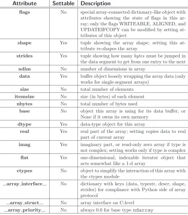
Table 3.1: Attributes of the ndarray.
Attribute
Settable
Description
flags No special array-connected dictionary-like object with attributes showing the state of flags in this ar-ray; only the flags WRITEABLE, ALIGNED, and UPDATEIFCOPY can be modified by setting at-tributes of this object
shape Yes tuple showing the array shape; setting this at-tribute re-shapes the array
strides Yes tuple showing how manybytes must be jumped in the data segment to get from one entry to the next
ndim No number of dimensions in array
data Yes buffer object loosely wrapping the array data (only works for single-segment arrays)
size No total number of elements
itemsize No size (in bytes) of each element nbytes No total number of bytes used
base No object this array is using for its data buffer, or None if it owns its own memory
dtype Yes data-type object for this array
real Yes real part of the array; setting copies data to real part of current array
imag Yes imaginary part, or read-only zero array if type is not complex; setting works only if type is complex flat Yes one-dimensional, indexable iterator object that
acts somewhat like a 1-d array
ctypes No object to simplify the interaction of this array with the ctypes module
array interface No dictionary with keys (data, typestr, descr, shape, strides) for compliance with Python side of array protocol
array struct No array interface on C-level
Certain logical combinations of flags can also be read using named keys to the special flags dictionary. These combinations are
FNC Returns F CONTIGUOUS and not C CONTIGUOUS
FORC Returns F CONTIGUOUS or C CONTIGUOUS (one-segment test). BEHAVED (B) Returns ALIGNED and WRITEABLE
CARRAY (CA) Returns BEHAVED and C CONTIGUOUS
FARRAY (FA) Returns BEHAVED and F CONTIGUOUS and not C CONTIGUOUS
NOTE
The array flags cannot be set arbitrarily. UPDATEIFCOPY can only be set False. the ALIGNED flag can only be set True if the data is truly aligned. The flag WRITEABLE can only be set True if the array owns its own memory or the ultimate owner of the memory exposes a writeable buffer interface (or is a string). The exception for string is made so that unpickling can be done without copying memory.
Flags can also be set and read using attribute access with the lower-case key equivalent (without first letter support). Thus, for example, self.flags.c contiguous returns whether or not the array is C-style contiguous, and self.flags.writeable=True changes the array to be writeable (if possible).
shape
NOTE
Setting the shape attribute to () for a 1-element array will turn self into a 0-dimensional array. This is one of the few ways to get a 0-dimensional array in Python. Most other operations will return an array scalar. Other ways to get a 0-dimensional array in Python include calling array with a scalar argument and calling the squeeze method of an array whose shape is all 1’s.
strides
The strides of an array is a tuple showing for each dimension how many bytes must be skipped to get to the next element in that dimension. Setting this attribute to another tuple will change the way the memory is viewed. This attribute can only be set to a tuple that will not cause the array to access unavailable memory. If an attempt is made to do so, ValueError is raised.
ndim
The number of dimensions of an array is sometimes called the rank of the array. Getting this attribute reveals the length of the shape tuple and the strides tuple.
data
A buffer object referencing the actual data for this array if this array is single-segment. If the array is not single-segment, then an AttributeError is raised. The buffer object is writeable depending on the status of self.flags.writeable.
size
The total number of elements in the array.
itemsize
The number of bytes each element of the array requires.
nbytes
The total number of bytes used by the array. This is equal to
If the array does not own its own memory, then this attribute returns the object whose memory this array is referencing. The returned object may not be the original allocator of the memory, but may be borrowing it from still another object. If this array does own its own memory, then None is returned unless the UPDATEIFCOPY flag is True in which case self.base is the array that will be updated when self is deleted. UPDATEIFCOPY gets set for an array that is created as a behaved copy of a general array. The intent is for the misaligned array to get any changes that occur to the copy.
3.1.2
Data Type attributes
There are several ways to specify the kind of data that the array is composed of. The fullest description that preserves field information is always obtained using an actual dtype object. See Chapter 7 for more discussion on data-type objects and acceptable arguments to construct data-type objects. Three commonly-used attri