ABSTRACT
HOUGH, ZACHARY CLARK.µ-bases and Algebraic Moving Frames: Theory and Computation. (Under the direction of Hoon Hong and Irina A. Kogan.)
We establish new results on the theory and computation ofµ-bases and algebraic moving frames for a vector of univariate polynomials, along with several related observations. First, we develop a new algorithm for computing aµ-basis of the syzygy module ofnpolynomials in one variable over an arbitrary fieldK. The algorithm is conceptually different from the previously-developed algorithms by Cox, Sederberg, Chen, Zheng, and Wang forn=3, and by Song and Goldman for an arbitrary n. The algorithm involves computing a “partial” reduced row-echelon form of a(2d+1)×n(d+1) matrix overK, whered is the maximum degree of the input polynomials. The proof of the algorithm is based on standard linear algebra and is completely self-contained. The proof includes a proof of the existence of theµ-basis and as a consequence provides an alternative proof of the freeness of the syzygy module. The theoretical (worst case asymptotic) computational complexity of the algorithm isO(d2n+d3+n2). We have implemented this algorithm (HHK) and the one developed
by Song and Goldman (SG). Experiments on random inputs indicate that SG is faster than HHK whend is sufficiently large for a fixedn, and that HHK is faster than SG whennis sufficiently large for a fixedd. We also develop a generalization of the HHK algorithm to compute minimal bases for the kernels ofm×npolynomial matrices.
We also characterize a relationship betweenµ-bases and Gröbner bases for the syzygy module of a vector ofnunivariate polynomials. Roughly put, we show that “everyµ-basis is a minimal TOP Gröbner basis” and that “every minimal TOP Gröbner basis is aµ-basis.” Precisely stated, we prove that, forU ⊂K[s]n, the following two statements are equivalent:
(A) U is aµ-basis of syz(a)
(B) U is a minimal TOPB-Gröbner basis of syz(a)for some ordered basisBofKn
where TOPB stands for the TOP ordering among the monomials defined byB.
Furthermore, we give an example showing thatnoteveryµ-basis is a TOPE-Gröbner basis, where
E stands for the standard basis ofKn. We prove that theµ-basis produced by the HHK algorithm is the reduced TOPE-Gröbner basis. We also give an example showing that not every minimal
POTB-Gröbner basis is aµ-basis.
Quillen-Suslin problem, effective Nullstellensatz problem, and syzygy module problem. The focus of these problems, however, is not degree optimality. By contrast, we develop the theory of and an efficient algorithm for constructing a degree-optimal moving frame. We also establish several new theoretical results concerning the degrees of an optimal moving frame and its components.
We develop a new degree-optimal moving frame (OMF) algorithm fornrelatively prime poly-nomials (i.e. gcd(a) =1). We develop a modification for the case when gcd(a)6=1. In addition, we show that any deterministic algorithm for computing a degree-optimal algebraic moving frame can be augmented so that it assigns a degree-optimal moving frame in aG Ln(K)-equivariant manner.
µ-bases and Algebraic Moving Frames: Theory and Computation
by
Zachary Clark Hough
A dissertation submitted to the Graduate Faculty of North Carolina State University
in partial fulfillment of the requirements for the Degree of
Doctor of Philosophy
Mathematics
Raleigh, North Carolina 2018
APPROVED BY:
Agnes Szanto Bojko Bakalov
Hoon Hong
Co-chair of Advisory Committee
Irina A. Kogan
DEDICATION
BIOGRAPHY
ACKNOWLEDGEMENTS
First and foremost, I want to thank my advisors, Hoon Hong and Irina Kogan, for making all of this possible. I have struggled to find the right words to express the full depth of my gratitude, so I will simply say thank you for your patience, your guidance, and your belief in me. You both have helped me to become a better mathematician, and I am incredibly grateful, on both a personal and professional level, for everything you have done for me. I also would like to thank my committee members, Agnes Szanto and Bojko Bakalov, as well as my GSR, Russell Philbrick, for their insight and assistance during this process. I’d also like to acknowledge grant US NSF CCF-1319632 for providing financial assistance at various points during my graduate studies.
I also want to thank my wonderful sister, Sarah, for being my best (and at times, only) friend throughout my life. In particular, over the last several years, you have provided humor, encourage-ment, and just the right amount of distraction as I worked toward this accomplishment. You are simply amazing.
TABLE OF CONTENTS
LIST OF FIGURES. . . vii
Chapter 1 Introduction. . . 1
Chapter 2 Review . . . 7
2.1 µ-bases . . . 7
2.1.1 Original definition . . . 8
2.1.2 Subsequent developments . . . 8
2.2 Algebraic moving frames . . . 12
2.2.1 Fitchas-Galligo algorithm . . . 12
2.2.2 Algorithm based on Euclidean division . . . 16
2.2.3 Fabianska-Quadrat algorithm . . . 17
Chapter 3 µ-bases. . . 18
3.1 An algorithm for computingµ-bases . . . 19
3.1.1 Definitions and problem statement . . . 19
3.1.2 Syzygies of bounded degree. . . 21
3.1.3 “Row-echelon” generators andµ-bases. . . 26
3.1.4 Algorithm . . . 34
3.1.5 Theoretical Complexity Analysis . . . 46
3.1.6 Implementation . . . 47
3.1.7 Experiments, timing, and fitting . . . 48
3.1.8 Comparison . . . 50
3.1.9 Original definition, homogeneous version, and gcd . . . 51
3.2 Matrix generalization: minimal bases . . . 53
3.3 Relationship betweenµ-bases and Gröbner bases . . . 58
3.3.1 Definitions . . . 59
3.3.2 Main result . . . 61
3.3.3 Everyµ-basis is a minimal TOP Gröbner basis . . . 61
3.3.4 Every minimal TOP Gröbner basis is aµ-basis . . . 65
Chapter 4 Algebraic moving frames: Theory . . . 67
4.1 Moving frames, Bézout vectors, and syzygies . . . 67
4.1.1 Basic definitions and notation . . . 68
4.1.2 Algebraic moving frames and degree optimality . . . 68
4.1.3 Bézout vectors . . . 69
4.1.4 Syzygies andµ-bases . . . 70
4.1.5 The building blocks of a degree-optimal moving frame . . . 73
4.1.6 The(β,µ)-type of a polynomial vector . . . 75
4.2 Reduction to a linear algebra problem overK . . . 77
4.2.1 Sylvester-type matrixAand its properties . . . 77
4.2.2 Isomorphism betweenK[s]mt andKm(t+1) . . . 79
4.2.3 The minimal Bézout vector theorem . . . 81
4.2.4 Theµ-bases theorem . . . 83
Chapter 5 Algebraic moving frames: Computation . . . 91
5.1 The OMF Algorithm . . . 92
5.1.1 Informal outline . . . 92
5.1.2 Formal algorithm and proof . . . 93
5.2 Case when gcd6=1 . . . 96
5.3 Equivariance . . . 102
5.4 Other approaches . . . 105
5.5 Fabianska-Quadrat algorithm . . . 106
5.6 Algorithm based on generalized extended GCD . . . 108
5.7 Unimodular multipliers . . . 110
5.8 Using POT Gröbner basis computations . . . 110
5.9 Using TOP Gröbner basis computations . . . 115
5.10 OMF viaµ-basis algorithm . . . 119
5.11 Matrix inputs . . . 120
LIST OF FIGURES
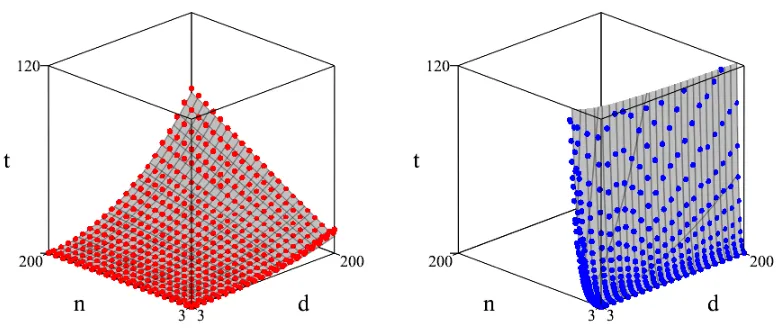
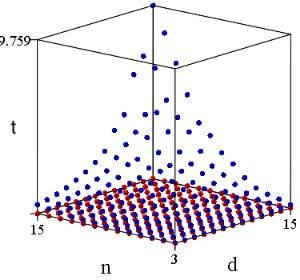
Figure 3.1 HHK algorithm timing . . . 49
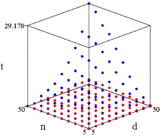
Figure 3.2 SG algorithm timing . . . 49
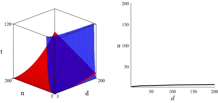
Figure 3.3 HHK (red) and SG (blue). . . 50
Figure 3.4 Tradeoff graph . . . 50
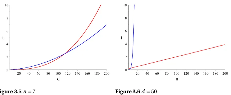
Figure 3.5 n=7 . . . 51
Figure 3.6 d =50 . . . 51
Figure 5.1 Timing comparison: OMF vs. Two-step approach . . . 107
CHAPTER
1
INTRODUCTION
The concept of aµ-basis for a vector of polynomials first appeared in[Cox98b], along with an algo-rithm for computing aµ-basis when the length of the input vector is three. Subsequent algorithms, also for the case when the input length is three, appeared in[ZS01]and[CW02]. The first algorithm for input vectors of arbitrary length appeared in[SG09]. These algorithms all require that the gcd of the input vector be 1, and they are described in greater detail in Chapter 2. In this work, one of our primary focuses is developing a new and alternative algorithm for computingµ-bases for vectors of arbitrary length and arbitrary gcd. Let us now motivate this development.
Consider a vectora[s] = [a1(s),a2(s), . . . ,an(s)]of univariate polynomials over an arbitrary fieldK. Such a vector will be our primary object of interest. Letnbe the length ofa, and letdbe the degree of a, by which we mean the maximum of the degrees of the component polynomialsai. It is well-known
that the syzygy module ofa, consisting of linear relations overK[s]amonga1(s), . . . ,an(s): syz(a) ={h∈K[s]n|a1h1+· · ·+anhn=0}
is free.1This means that the syzygy module has a basis, and, in fact, infinitely many bases. Moreover, if one viewsaas a parametric curve, then one can take a basis of syz(a)and use it as a set of moving lines whose intersections trace out the curve. Aµ-basis is a basis with particularly nice properties, which make the problem of finding aµ-basis an important one to study. Namely, aµ-basis is a minimal-degree basis of syzygies. Additional nice properties thatµ-bases provide include point-wise linear independence (i.e. linear independence at alls0in the algebraic closureK) and independence of
1Freeness of the syzygy module in the one-variable case can be deduced from the Hilbert Syzygy Theorem[Hil90]. In
leading vectors, among others. Furthermore,µ-bases have nice applications in geometric modelling. In addition to giving one a means to represent a curve as described above,µ-bases also allow one to classify curves (see[CI15]). Specifically, although aµ-basis is not unique, the degrees of theµ-basis are unique, so one can partition the collection ofµ-bases by degrees, which then induces a partition on the collection of curves. Aµ-basis also can be used to find the implicit equation of a curve, to determine if and where two curves intersect, and to determine if a point lies on a curve, among other applications. It is more computationally efficient to useµ-bases in these instances than other bases of syzygies due to their minimal-degree property.
These applications and properties motivate the development of efficient algorithms for comput-ingµ-bases. In this work, we develop a new algorithm for computingµ-bases for input vectors of arbitrary length and arbitrary GCD. We now briefly describe the main ideas behind our algorithm. It is well-known that the syzygy module ofa, syz(a), is generated by the set syzd(a)of syzygies of degree at mostd=deg(a). The set syzd(a)is obviously aK-subspace ofK[s]n. Using the standard monomial basis, it is easy to see that syzd(a)is isomorphic to the kernel of a certain linear map A:Kn(d+1)→K2d+1(explicitly given by (3.7)). Now we come to thekeyidea: one cansystematically choose a suitable finite subset of the kernel ofAso that the corresponding subset of syzd(a)forms a µ-basis. We elaborate on how this is done. Recall that a column of a matrix is callednon-pivotal if it is either the first column and zero, or it is a linear combination of the previous columns. Now we observe and prove a remarkable fact: the set of indices of non-pivotal columns ofAsplits into exactlyn−1 sets of modulo-n-equivalent integers. By taking the smallest representative in each set, we obtainn−1 integers, which we callbasic non-pivotalindices. The set of non-pivotal indices ofA is equal to the set of non-pivotal indices of its reduced row-echelon formE. From each non-pivotal column ofE, an element of ker(A)can easily be read off, that, in turn, gives rise to an element of syz(a), which we calla row-echelon syzygy. We prove that the row-echelon syzygies corresponding to then−1basic non-pivotalindices comprise aµ-basis. Thus, aµ-basis can be found by computing the reduced row-echelon form of a single(2d+1)×n(d+1)matrixAoverK. Actually, it is sufficient to compute only a “partial” reduced row-echelon form containing only the basic non-pivotal columns and the preceding pivotal columns.
Performance-wise, our algorithm compares favorably to existing approaches. We show that the new algorithm has theoretical complexityO(d2n+d3+n2), assuming that the arithmetic takes constant time (which is the case when the fieldKis finite). We have implemented our algorithm (HHK), as well as Song and Goldman’s[SG09]algorithm (SG) in Maple[Ber15]. Experiments on random inputs indicate that SG is faster than HHK whend is sufficiently large for a fixednand that HHK is faster than SG whennis sufficiently large for a fixedd.
The problem of computing aµ-basis also can be viewed as a particular case of the problem of computing optimal-degree bases for the kernels ofm×npolynomial matrices (see for instance Beelen[Bee87], Antoniou, Vardulakis, and Vologiannidis[Ant05], Zhou, Labahn, and Storjohann
The algorithm works for matrices of arbitrary size and rank, and as a by-product it can be used to compute the rank of the input matrix.
Let us now turn our attention to algebraic moving frames[Hon18]. As mentioned above, a nonzero row vectora ∈ K[s]n defines a parametric curve inKn. The columns of a matrixP ∈ G Ln(K[s])assign a basis of vectors inKn at each point of the curve. Here,G Ln(K[s])denotes the
set of invertiblen×nmatrices overK[s], or equivalently, the set of matrices whose columns are point-wiselinearly independent over the algebraic closureK. In other words, the columns of the matrixP can be viewed as a coordinate system, or a frame, that moves along the curve. To be of interest, however, such assignment should not be arbitrary, but instead be related to the curve in a meaningful way. From now on, we require thataP = [gcd(a), 0, . . . , 0], where gcd(a)is the monic greatest common divisor of the components ofa. We will call a matrixP with the above property analgebraic moving frame ata. We observe that for any nonzero monic polynomialλ(s), a moving frame atais also a moving frame atλa. Therefore, we can obtain an equivalent construction in the projective spacePKn−1by considering only polynomial vectorsasuch that gcd(a) =1. ThenP can be thought of as an element ofP G Ln(K[s]) =G Ln(K[s])/c I, wherec 6=0∈KandI is an identity matrix. A canonical map ofato any of the affine subsetsKn−1⊂PKn−1produces a rational curve in Kn, andP assigns a projective moving frame ata. We are particularly interested indegree-optimal algebraic moving frames – frames that column-wise have minimal degrees, where the degree of a column is defined to be the maximum of the degrees of its components (see Definitions 6 and 63). The problem of finding a degree-optimal algebraic moving frame is worthwhile to study for various reasons. First of all, it is clear that the first column of an algebraic moving frameP satisfies aP∗1=gcd(a). That is, the first column is a Bézout vector ofa, a vector comprised of the coefficients
appearing in the output of the extended Euclidean algorithm. Thus, the first column of a degree-optimal moving frame is a minimal-degree Bézout vector. Our literature search did not yield any efficient algorithm for computing a minimal-degree Bézout vector. Of course, one can compute such a vector by a brute-force method, namely by searching for a Bézout vector of a fixed degree, starting from degree zero, increasing the degree by one, and terminating the search once a Bézout vector is found, but this procedure is very inefficient. As such, computing a degree-optimal moving frame would allow for a more efficient computation of a minimal-degree Bézout vector. Secondly, it is obvious that the lastn−1 columns of an algebraic moving frameP are syzygies ofa. In Proposition 68, we prove that these lastn−1 columns ofP comprise a point-wise linearly independent basis of the syzygy module ofa. Thus, the lastn−1 columns of a degree-optimal moving frame form a basis of the syzygy module ofaofoptimal degree, i.e. aµ-basis. As mentioned above,µ-bases have a long history of applications in geometric modeling, originating with works by Sederberg and Chen
differential degrees of “flat outputs” (see, for instance, Polderman and Willems[PW98], Martin, Murray and Rouchon[Mar01], Fabia ´nska and Quadrat[FQ07], Antritter and Levine[AL10], Imae, Akasawa, and Kobayashi[Ima15]). Another interesting application of algebraic frames can be found in the paper[Elk12]by Elkadi, Galligo and Ba, devoted to the following problem: given a vector of polynomials with gcd 1, find small degree perturbations so that the perturbed polynomials have a large-degree gcd. As discussed in Example 3 of[Elk12], the perturbations produced by the algorithm presented in this paper do not always have minimal degrees. It would be worthwhile to study if the usage of degree-optimal moving frames can decrease the degrees of the perturbations.
The applications available to degree-optimal moving frames motivate the development of efficient algorithms for their construction. Algebraic moving frames appeared in a number of important proofs and constructions under a variety of names. For example, in the constructive proofs of the celebrated Quillen-Suslin theorem[FG90],[LS92],[Can93],[PW95],[LY05],[FQ07], given a polynomialunimodularm×nmatrixA, one constructs a unimodular matrixP such that AP = [Im,0], whereImis anm×midentity matrix. In the univariate case withm=1, the matrixP is an algebraic moving frame. However, the above works were not concerned with the problem of findingP of optimal degree for every inputA. We describe these approaches in greater detail in Chapter 2.
n=3 case, and by Song and Goldman[SG09]and Hong, Hough and Kogan[Hon17]for arbitraryn. As mentioned previously, the problem of computing aµ-basis also can be viewed as a particular case of the problem of computing optimal-degree bases for the kernels ofm×npolynomial matrices. Algorithms for this problem have been developed by Beelen[Bee87], Antoniou, Vardulakis, and Vologiannidis[Ant05], Zhou, Labahn, and Storjohann[Zho12]. However, these approaches are insufficient due to the lack of an efficient method for computing minimal-degree Bézout vectors.
Alternatively, one can first construct a non-optimal moving frame by algorithms using, for instance, a generalized version of Euclid’s extended gcd algorithm, as described by Polderman and Willems in[PW98], or various algorithms presented in the literature devoted to the constructive Quillen-Suslin theorem and the related problem of unimodular completion: Fitchas and Galligo
[FG90], Logar and Sturmfels[LS92], Caniglia, Cortiñas, Danón, Heintz, Krick, and Solernó[Can93], Park and Woodburn[PW95], Lombardi and Yengui[LY05], Fabia ´nska and Quadrat[FQ07], Zhou-Labahn[ZL14]. Then a degree-reduction procedure can be performed, for instance, by computing the Popov normal form of the lastn−1 columns of a non-optimal moving frame, as discussed in
[Bec06], and then reducing the degree of its first column. We discuss this approach in Section 5.4, and demonstrate that it is less efficient than the direct algorithm based on the theory from Sections 4.1 and 4.2 and presented in Section 5.1.
In addition to developing the theory behind an algorithm for computing an optimal moving frame, we prove new results about the degrees of optimal moving frames and its building blocks. These degrees play an important role in the classification of rational curves, because although a degree-optimal moving frame is not unique, its columns have canonical degrees. The list of degrees of the lastn−1 columns (µ-basis columns) is called theµ-type of an input polynomial vector, and µ-strata analysis was performed in D’Andrea[D’A04], Cox and Iarrobino[CI15]. In Theorem 76, we show that the degree of the first column (Bézout vector) is bounded by the maximal degree of the other columns, while Proposition 77 shows that this is the only restriction that theµ-type imposes on the degree of a minimal Bézout vector. Thus, one can refine theµ-strata analysis to the (β,µ)-strata analysis, whereβdenotes the degree of a minimal-degree Bézout vector. This work can have potential applications to rational curve classification problems. In Proposition 92 and Theorem 96, we establish sharp lower and upper bounds for the degree of an optimal moving frame and show that for a generic vectora, the degree of an optimal moving frame equals to the sharp lower bound.
CHAPTER
2
REVIEW
In this chapter, we provide a more thorough review of the previous work onµ-bases and algebraic moving frames. In particular, we examine some of the previous algorithms for their construction, along with other related observations.
2.1
µ
-bases
As mentioned in the Chapter 1, one of the main problems we consider is the problem of computing a µ-basis for a vectoraof univariate polynomials. The concept of aµ-basis first appeared in[Cox98b], motivated by the search for new, more efficient methods for solving implicitization problems for rational curves, and as a further development of the method of moving lines (and, more generally, moving curves) proposed in[SC95]. Since then, a large body of literature on the applications of µ-bases to various problems involving vectors of univariate polynomials has appeared, such as
[Che05; SG09; JG09; TW14].1The variety of possible applications motivates the development of
algorithms for computingµ-bases. Although a proof of the existence of aµ-basis for arbitraryn appeared already in[Cox98b], the algorithms were first developed for then=3 case only[Cox98b; ZS01; CW02]. The first algorithm for arbitrarynappeared in[SG09], as a generalization of[CW02]. We now review some of these approaches.
1A notion of aµ-basis for vectors of polynomials in two variables also has been developed and applied to the study
of rational surfaces in three-dimensional projective space (see, for instance,[Che05; Shi12]). We focus solely on the
2.1.1 Original definition
The original definition of aµ-basis appeared on p 824 of a paper by Cox, Sederberg, and Chen
[Cox98b]. Given a vectora∈K[s]nwith gcd(a) =1 and deg(a) =d, aµ-basis ofais a generating set
u1, . . . ,un−1of syz(a)satisfying deg(u1) +· · ·+deg(un−1) =d. In the paper, the degrees ofu1, . . . ,un−1
were denotedµ1, . . . ,µn−1, and the termµ-basis was coined. Also in the paper, the authors prove
that aµ-basis always exists for vectors of arbitrary length. The proof of the existence theorem (Theorem 1 on p. 824 of[Cox98b]) appeals to the celebrated Hilbert Syzygy Theorem[Hil90]and utilizes Hilbert polynomials, which first appeared in the same paper[Hil90]under the name of characteristic functions.
The proof of existence for vectors of arbitrarynis non-constructive. However, the authors of
[Cox98b]do implicitly suggest an algorithm for then=3 case. Later, it was explicitly described in the Introduction of[ZS01]. The algorithm relies on the fact that, in then=3 case, there are only two elements in aµ-basis, and their degrees (denoted asµ1andµ2) can be determinedpriorto
computing the basis (see Corollary 2 on p. 811 of[Cox98b]and p. 621 of[ZS01]). Once the degrees are determined, two syzygies are constructed from null vectors of two linear mapsA1:K3(µ1+1)→
Kµ1+d+1andA2:K3(µ2+1)→Kµ2+d+1. Special care is taken to ensure that these syzygies are linearly independent overK[s]. These two syzygies comprise aµ-basis. It is not clear, however, how this method can be generalized to arbitraryn. First, as far as we are aware, there is not yet an efficient way to determine the degrees ofµ-basis membersa priori. Second, there is not yet an efficient way for choosing appropriate null vectors so that the resulting syzygies are linearly independent.
2.1.2 Subsequent developments
The next approach we review is by Zheng and Sederberg[ZS01], who gave a different (more efficient) algorithm for then=3 case, based on Buchberger-type reduction. The algorithm makes use of the fact that, when gcd(a) =1, the three obvious syzygies[a2,−a1, 0],[a3, 0,−a1], and[0,a3,−a2]generate
syz(a). Then Buchberger-type reduction is used to reduce the degree of one of the syzygies at a time. This is done until one of the syzygies reduces to 0, after which the remaining two syzygies comprise aµ-basis. Here, we provide the details of the algorithm. Note, the notationLT refers to the leading term of a polynomial vector. A term of a vector inK[s]nisc skei, wherec is a constant andeiis the
i-th standard basis vector. The leading term of a vector is the term of highest degree and highest position, while the constant in the leading term is called the leading coefficient and denotedLC.
Input:a∈K[s]3with gcd(a) =1
Output: Aµ-basis ofa
1. u1= [a2,−a1, 0]T,u2= [a3, 0,−a1]T,u3= [0,a3,−a2]T
3. Replaceuiwith
ui←−
LC M(LC(ui),LC(uj))
LC(ui)
ui−
LC M(LC(ui),LC(uj))
LC(uj)
sdeg(ui)−deg(uj)u
j
whereLC M represents the least common multiple.
4. Ifui=0, output remaining nonzero vectors. Else go to step 2.
Example 1. We demonstrate the update procedure ona=1+s2, 2+s2, 3+s2
. Start with
u1=
2+s2 −1−s2
0
, u2=
3+s2 0 −1−s2
, u3=
0 3+s2 −2−s2
.
1. Since LT(u1) =s2e1and LT(u2) =s2e1, we update
u1=u1−u2=
−1 −1−s2
1+s2
.
2. Since LT(u1) =−s2e2and LT(u3) =s2e2, we update
u1=u1+u3=
−1 2 −1
.
3. Since LT(u1) =−e1and LT(u2) =s2e1, we update
u2=u2+s2u1=
3 2s2
−1−2s2
.
4. Since LT(u2) =2s2e2and LT(u3) =s2e2, we update
u2=u2−2u3=
3 −6
3
.
5. Since LT(u1) =−e1and LT(u2) =3e1, we update
u2=u2+3u1=
0 0 0
We then output theµ-basis
−1 2 −1
,
0 3+s2
−2−s2
.
A more efficient modification of this procedure was proposed by Chen and Wang[CW02], where instead of reducing based on leading terms, the reduction is done using relationships among leading vectors. Note, the degree of a polynomial vectorhis the maximum of the degrees of its components, and the leading vector is the vector of deg(h)coefficients. Here, we provide the details of the algorithm.
Input:a∈K[s]3with gcd(a) =1
Output: Aµ-basis ofa
1. u1= [a2,−a1, 0]T,u2= [a3, 0,−a1]T,u3= [0,a3,−a2]T
2. Setmi=LV(ui)anddi=deg(ui)fori=1, 2, 3.
3. Sortdiso thatd1≥d2≥d3and re-indexui,mi.
4. Find real numbersα1,α2,α3such thatα1m1+α2m2+α3m3=0.
5. Ifα16=0, updateu1by
u1=α1u1+α2sd1−d2u
2+α3sd1−d3u3
and updatem1andd1accordingly. Ifα1=0, updateu2by
u2=α2u2+α3sd2−d3u 3
and updatem2andd2accordingly.
6. If one of the vectors is zero, then output the remaining nonzero vectors and stop; otherwise, go to Step 3.
Example 2. We demonstrate the modified update procedure ona=1+s2, 2+s2, 3+s2. Start with
u1=
2+s2
−1−s2 0
, u2=
3+s2
0 −1−s2
, u3=
0 3+s2 −2−s2
.
1. Since m1=LV(u1) = [1,−1, 0]T, m2=LV(u2) = [1, 0,−1]T, and m3=LV(u3) = [0, 1,−1]T, we
haveα1=1,α2=−1, andα3=1, so we update
u1=u1−u2+u3=
−1 2 −1
and re-index
u1=
3+s2 0 −1−s2
,u2=
0 3+s2 −2−s2
,u3=
−1 2 −1 .
2. Since m1= [1, 0,−1]T, m
2= [0, 1,−1]T, and m3= [−1, 2,−1]T, we haveα1=1,α2=−2, and
α3=1, so we update
u1=u1−2u2+s2u3= 3 −6 3 and re-index
u1=
0 3+s2 −2−s2
, u2=
3 −6 3 ,u3=
−1 2 −1 .
3. Since m1= [0, 1,−1]T, m2= [3,−6, 3]T, and m3= [−1, 2,−1]T, we haveα1=0,α2=1, andα3=3,
so we update
u2=u2+3u3= 0 0 0 .
We then output theµ-basis
−1 2 −1 , 0 3+s2 −2−s2
.
Observe that the modified procedure using leading vectors works in fewer steps than the original procedure using leading terms. The algorithm in[CW02]was subsequently generalized to arbitrary nby Song and Goldman[SG09]. The general algorithm starts by observing that the set of the obvious syzygies{[ −aj ai ]|1≤i<j≤n}generates syz(a), provided gcd(a) =1. Then Buchberger-type
reduction is used to reduce the degree of one of the syzygies at a time. It is proved that when such reduction becomes impossible, one is left with exactlyn−1 non-zero syzygies that comprise a µ-basis. If gcd(a)is non-trivial, then the output is aµ-basis multiplied by gcd(a). The full details of the algorithm are below.
Input:a∈K[s]nwith gcd(a) =1
Output: Aµ-basis ofa
1. Create ther =C2n “obvious" syzygies and label themu1, . . . ,ur.
2. Setmi=LV(ui)anddi=deg(ui)fori=1, . . . ,r.
4. Find real numbersα1,α2, . . . ,αr such thatα1m1+α2m2+· · ·+αrmr=0.
5. Choose the lowest integer jsuch thatαj 6=0, and updateuj by setting
uj =αjuj+αj+1sdj−dj+1uj+1+· · ·+αrsdj−drur.
Ifuj≡0, discarduj and setr=r −1; otherwise setmj=LV(uj)anddj =deg(uj).
6. Ifr =n−1, then output then−1 non-zero vector polynomialsu1, . . . ,un−1and stop; otherwise,
go to Step 3.
2.2
Algebraic moving frames
The other main problem we consider is that of computing a degree-optimal algebraic moving frame at a vectoraof univariate polynomials. An algebraic moving frame ata∈K[s]n is a matrix
P ∈G Ln(K[s])such thataP = [gcd(a), 0, . . . , 0]. A degree-optimal moving frame has minimal
column-wise degree. The problem of constructing an algebraic moving frame is a particular case of the well-known problem of providing a constructive proof of the Quillen-Suslin theorem[FG90],[LS92],
[Can93],[PW95],[LY05],[FQ07]. In those papers, the multivariate problem is reduced inductively to the univariate case, and then an algorithm for the univariate case is proposed. Those univariate algorithms produce algebraic moving frames. As far as we are aware, the produced moving frames areusually notdegree-optimal. However, the algorithms are very efficient. We now review some of these approaches.
2.2.1 Fitchas-Galligo algorithm
We start by discussing an algorithm that appeared in[FG90]by Fitchas and Galligo. Before presenting the algorithm, however, we need the following lemma.
Lemma 3. Let n ≥3. Leta= [a1, . . . ,an]∈K[s]n be such thatgcd(a1, . . . ,an) =1. Then there exist
k3, . . . ,kn∈Ksuch thatgcd(a1+k3a3+· · ·+knan,a2) =1.
Proof. Letd be the degree ofa2. Letβ1, . . . ,βd be the roots ofa2 in the algebraic closure ofK. Consider the following set
C =Kn−2\ (S1∪ · · · ∪Sd)
where
Si=
(k3, . . . ,kn)∈Kn−2|a1 βi
+k3a3 βi
+· · ·+knan βi
=0 . The lemma is immediate from the following claims.
1. dimC=n−2≥1.
Proof: Note thatSiis aK-affine space. Since gcd(a1, . . . ,an) =1, for everyi∈ {1, . . . ,d}, at least
one of the following is non-zero:a1 βi
,a3 βi
, . . . ,an β
. Thus dimSi≤n−3. In turn dim
2. ∀(k3, . . . ,kn)∈C gcd(a1+k3a3+· · ·+knan,a2) =1.
Proof: Let(k3, . . . ,kn)∈C. Then for everyi∈ {1, . . . ,d}, we have
a1 βi
+k3a3 βi
+· · ·+knan βi
6=0.
Thus
gcd(a1+k3a3+· · ·+knan,a2) =1.
We remark that finding the constantskias described in the lemma can be completed with a random search. Moreover, for random inputs, gcd(a1,a2) =1 and one can take eachki=0.
Now,[FG90]describes the following general algorithm for the univariate case: 1. FindM ∈K[s]n×nwith|M|=1 such thataM =a(0).
2. FindT ∈Kn×n with|T|=1 such thata(0)T = [1, 0, . . . , 0]. 3. P =M T.
To find matrixM, they do the following. Assumea1anda2are relatively prime (otherwise, find
constants as described in Lemma 3). Then there existf1,f2∈K[s]such thata1f1+a2f2=1.
Define
A=
f1(s) −a2(s) f1(s)[a3(0)−a3(s)] · · · f1(s)[an(0)−an(s)] f2(s) a1(s) f2(s)[a3(0)−a3(s)] · · · f2(s)[an(0)−an(s)]
1
...
1
.
ThenaA= [1, 0,a3(0), . . . ,an(0)]and|A|=1. Define
B=
a1(0) a2(0)
−f2(0) f1(0)
1 ...
1
.
Then[1, 0,a3(0), . . . ,an(0)]B= [a1(0),a2(0),a3(0), . . . ,an(0)]and|B|=1.
LetM =AB. ThenaM =a(0)and|M|=1.
Lemma 4. Let i be any such thata(0)i6=0.Let j be any such that1≤j≤n and j6=i.Let
ˆ ek=
¨
ek if k6=j (−1)1+i
a(0)i ek if k=j where ek is the k -th standard unit (row) vector. Finally let
T = a(0) ˆ e1 .. . ˆ ei−1
ˆ ei+1
.. . ˆ en −1 .
Thena(0)T = 1 0 · · · 0 and
T =1.
Proof. For the first claim, we observe that
a(0)T =
1 0 · · · 0
a(0) ˆ e1
.. . ˆ ei−1
ˆ ei+1
.. . ˆ en T =
1 0 · · · 0 T−1T = 1 0 · · · 0 T−1T = 1 0 · · · 0 . To show the second claim, consider
T −1 =
a(0) ˆ e1
.. . ˆ ei−1
ˆ ei+1
.. . ˆ en
=(−1)
1+i
a(0)i
a(0) e1
.. . ei−1 ei+1
.. . en .
properties of the determinant, we get T −1 =
(−1)1+i a(0)i
a(0)iei
e1
.. . ei−1
ei+1
.. . en = e1 .. . ei−1
ei
ei+1
.. . en =1. Therefore T =1.
We now present the Fitchas-Galligo algorithm.
Input:a6=0∈K[s]nwith gcd(a) =1
Output: A moving frame ata
1. Find constantsk3, . . . ,knsuch that gcd(a1+k3a3+· · ·+knan,a2) =1.
2. Find f1,f2∈K[s]such that(a1+k3a3+· · ·+knan)f1+a2f2=1. This can be done by using the Extended Euclidean Algorithm.
3. M ←−K AB, where
K = 1 1
k3 1
..
. ...
kn 1
A=
f1 −a2 f1[a3(0)−a3] · · · f1[an(0)−an]
f2 a10 f2[a3(0)−a3] · · · f2[an(0)−an]
1 ... 1 B=
a10(0) a2(0)
−f2(0) f1(0)
1 ... 1 ,
4. Find matrixT such thata0(0)T = [1, 0, . . . , 0] (wherea0= [a10,a2, . . . ,an]).
(a) i←−such thata0(0)i6=0
(b) j←−such that 1≤j≤nandj6=i (c) ˆek =
¨
ek if k 6=j
(−1)1+i/a0(0)iek if k =j
whereekis thek-th standard unit (row) vector
(d) T ←−
a0(0) ˆ e1
.. . ˆ ei−1
ˆ ei+1
.. . ˆ en
−1
5. P ←−M T
The proof of the algorithm is immediate from the fact thataP =aM T =a0(0)T = [1, 0, . . . , 0]and |P|=|M T|=|M||T|=1.
2.2.2 Algorithm based on Euclidean division
Another simple and elegant algorithm for constructing not-necessarily-optimal moving frames, based on a generalized version of Euclid’s extended gcd algorithm, was first mentioned in[LS92]and
[PW95]. The authors did not explicitly describe the algorithm, though. However, it can be extracted from Theorem B.1.16 of the book “Introduction to the Mathematical Theory of Systems and Control” by Polderman and Willems[PW98], and it later appeared in[Elk12]as well. We present it here, and we denote it MF_GE (for Moving Frame by Generalized Euclid’s algorithm).
Input: a∈K[s]n,a6=0
Output:P, a moving frame ata
1. Letk be such thata= a1 · · · ak 0 · · · 0
whereak6=0.
2. Ifk=1 then set
P =
1 lc(a1)
1 ...
1
and returnP. (Here, lc(a1)denotes the leading coefficient ofa1.)
(a) r ←a1
(b) Fori=2, . . . ,k do qi←quo(r,ai)
r←rem(r,ai)
4. a0← a2 · · · ak r 0 · · · 0
.
5. T ←
1
1 −q2
... ... 1 −qk
1 ... 1
∈K[s]n×n,
where theq’s are placed in thek-th column 6. P0←MF_GE(a0).
7. P ←T P0. 8. ReturnP.
The proof of the algorithm is immediate from the fact that, at each step of the algorithm,aT =a0 and|T|=1.
2.2.3 Fabianska-Quadrat algorithm
Another very efficient algorithm for constructing not-necessarily-optimal algebraic moving frames appeared in[FQ07]. We present it here.
Input:a6=0∈K[s]nwith gcd(a) =1
Output: A moving frame ata
1. Find constantsk3, . . . ,knsuch that gcd(a1+k3a3+· · ·+knan,a2) =1.
2. Find f1,f2∈K[s]such that(a1+k3a3+· · ·+knan)f1+a2f2=1. This can be done by using the
Extended Euclidean Algorithm.
3. P ←−
1 1
k3 1
..
. ...
kn 1
f1 −a2 f2 a10
1 ... 1
1 0 −a3 · · · −an
0 1 1 ... 1 ,
wherea10=a1+k3a3+· · ·+knan.
CHAPTER
3
µ
-BASES
This chapter examines both the theory and computation ofµ-bases. In Section 3.1, we present a new and alternative algorithm for computing aµ-basis for vectors of arbitrary lengthn. The proof of the algorithm does not rely on previously established theorems about the freeness of the syzygy module or the existence of aµ-basis, and, therefore, as a by-product, provides an alternative, self-contained, constructive proof of these facts. Before presenting the algorithm, we give a rigorous definition of a µ-basis, describe its characteristic properties, and formulate the problem of computing aµ-basis. We prove several lemmas about the vector space of syzygies of degree at mostd, and the role they play in generating the syzygy module. We define the notion ofrow-echelon syzygiesand explain how they can be computed. We then present our main theoretical result, Theorem 31, which explicitly identifies a subset ofrow-echelon syzygiesthat comprise aµ-basis. We present an algorithm for computing aµ-basis, we analyze the theoretical (worst case asymptotic) computational complexity of this algorithm, we discuss implementation and experiments, and we compare the performance of the algorithm presented here with the one described in[SG09].
In Section 3.2, we consider a natural generalization of theµ-basis problem. Namely, that of considering kernels, or nullspaces, ofm×npolynomial matrices. An optimal degree basis of the nullspace is called a minimal basis. We show that theµ-basis algorithm presented in this chapter can be generalized to compute minimal bases of the kernels ofm×npolynomial matrices.
In Section 3.3, we characterize an interesting relationship betweenµ-bases and Gröbner bases of the syzygy module. We define monomial orderings onK[s]n and highlight two in particular, TOP
and POT. We provide a background on Gröbner bases for a submodule inK[s]n. We then show
µ-basis. We also show that theµ-basis algorithm presented in this chapter produces aµ-basis that is the reduced TOP Gröbner basis of the syzygy module relative to the standard basis ofKn. We also give an example showing that not every minimal POT Gröbner basis is aµ-basis.
3.1
An algorithm for computing
µ
-bases
In this section, we provide a background onµ-bases, develop the theory of a newµ-basis algorithm, present a new algorithm for computing aµ-basis, analyze the theoretical complexity of the algorithm, and compare the algorithm with the one described in[SG09].
3.1.1 Definitions and problem statement
As mentioned previously,Kdenotes a field andK[s]denotes a ring of polynomials in one indetermi-nates. The symbolnwill be reserved for the length of the polynomial vectora, whose syzygy module we are considering, and from now on we assumen>1, because for then=1 case the problem is trivial. The symbold is reserved for the degree ofa. We also will assume thatais anon-zero vector. All vectors are implicitly assumed to becolumn vectors, unless specifically stated otherwise. Superscript T denotes transposition.
Definition 5(Syzygy). Leta= [a1, . . . ,an]∈K[s]n be arown -vector of polynomials. Thesyzygyset of
ais
syz(a) ={h∈K[s]n|a h=0}.
We emphasize thathis by default a column vector andais explicitly defined to be a row vector, so that the producta his well-defined. It is easy to check that syz(a)is aK[s]-module. To define a µ-basis, we need the following terminology:
Definition 6(Leading vector). Forh∈K[s]n we define thedegreeand theleading vectorofhas follows:
• deg(h) = max
i=1,...,ndeg(hi).
• LV(h) = [coeff(h1,t), . . . , coeff(hn,t)]T ∈ Kn, where t = deg(h)andcoeff(hi,t)denotes the
coefficient of st in hi.
Example 7. Leth=
1−2s−2s2−s3
2+2s+s2+s3 −3
. Thendeg(h) =3and LV(h) =
−1 1 0
.
Before giving the definition of aµ-basis, we state a proposition that asserts the equivalence of several statements, each of which can be taken as a definition of aµ-basis.
Proposition 8. For a subset u={u1, . . . ,un−1} ⊂syz(a), ordered so thatdeg(u1)≤ · · · ≤deg(un−1), the
1. [independence of the leading vectors]The set u generatessyz(a), and the leading vectors LV(u1), . . . ,LV(un−1)are independent overK.
2. [minimality of the degrees]The set u generatessyz(a), and ifh1, . . . ,hn−1is any generating set
ofsyz(a), such thatdeg(h1)≤ · · · ≤deg(hn−1), thendeg(ui)≤deg(hi)for i=1, . . . ,n−1.
3. [sum of the degrees]The set u generatessyz(a), anddeg(u1)+· · ·+deg(un−1) =deg(a)−deg(gcd(a)).
4. [reduced representation]For everyh∈syz(a), there exist g1, . . . ,gn−1∈K[s]such thatdeg(gi)≤
deg(h)−deg(ui)and
h=
n−1 X
i=1
giui. (3.1)
5. [outer product]There exists a non-zero constantα∈Ksuch that the outer product ofu1, . . . ,un−1
is equal toαa/gcd(a).
Here and below gcd(a)denotes the greatest common monic devisor of the polynomialsa1, . . . ,an. The above proposition is a slight rephrasing of Theorem 2 in[SG09]. The only notable difference is that we drop the assumption that gcd(a) =1 and modify Statements 3 and 5 accordingly. After making an observation that syz(a) =syz a/gcd(a), one can easily check that a proof of Proposition 8 can follow the same lines as the proof of Theorem 2 in[SG09].We do not use Proposition 8 to derive and justify our algorithm for computing aµ-basis, and therefore we are not including its proof. However, we do prove some of these properties in Section 4.2.4. We include this proposition to underscore several important properties of aµ-basis and to facilitate comparison with the previous work on the subject.
Following[SG09], we base our definition of aµ-basis on Statement 1 of Proposition 8. We are making this choice, because in the process of proving the existence of aµ-basis, we explicitly construct a set ofn−1 syzygies for which Statement 1 can be easily verified, while verification of the other statements of Proposition 8 is not immediate. The original definition of aµ-basis (p. 824 of
[Cox98b]) is based on the sum of the degrees property (Statement 2 of Proposition 8). In Section 3.1.9, we discuss the advantages of the original definition.
Definition 9(µ-basis). For a non-zero row vectora∈K[s]n, a subset u⊂K[s]n of polynomial vectors
is called aµ-basis ofa, or, equivalently, aµ-basis ofsyz(a), if the following three properties hold: 1. u has exactly n−1elements.
2. LV(u1), . . . ,LV(un−1)are independent overK. 3. u is a basis ofsyz(a), the syzygy module ofa.
In the next two sections, through a series of lemmas culminating in Theorem 31, we give a self-contained constructive proof of the existence of aµ-basis. This, in turn, leads to an algorithm, presented in Section 3.1.4, for solving the following problem:
Problem:
Input: a6=0∈K[s]n, row vector, wheren>1 andKis a computable field1 Output: M ∈K[s]n×(n−1), such that the columns ofM form aµ-basis ofa
Example 10(Running example). We will be using the following simple example throughout this section to illustrate the theoretical ideas/findings and the resulting algorithm.
Input: a= 1+s2+s4 1+s3+s4 1+s4 ∈Q[s]3
Output: M =
−s 1−2s−2s2−s3
1 2+2s+s2+s3
−1+s −3
In contrast to the algorithm developed by Song and Goldman in[SG09], the algorithm presented in this section produces aµ-basis even when the input vectorahas a non-trivial greatest common divisor (see Section 3.1.9 for more details).
It is worthwhile emphasizing that not every basis of syz(a)is aµ-basis. Indeed, letu1andu2be
the columns of matrixM in Example 10. Thenu1+u2andu2is a basis of syz(a), but not aµ-basis,
becauseLV(u1+u2) =LV(u2). Aµ-basis is not canonical: for instance,u1andu1+u2will provide
anotherµ-basis for syz(a)in Example 10. However, Statement 2 of Proposition 8 implies that the degrees of the members of aµ-basis are canonical. In[Cox98b], these degrees were denoted by µ1, . . . ,µn−1and the term “µ-basis” was coined. A more in-depth comparison with previous works
onµ-bases and discussion of some related problems can be found in Section 3.1.9.
3.1.2 Syzygies of bounded degree.
From now on, let〈〉K[s]stand for theK[s]-module generated by. It is known that syz(a)is generated by polynomial vectors of degree at mostd =deg(a). To keep our presentation self-contained, we provide a proof of this fact (adapted from Lemma 2 of[SG09]).
Lemma 11. Leta∈K[s]nbe of degree d . Thensyz(a)is generated by polynomial vectors of degree at most d .
Proof. Let ˜a=a/g c d(a) = [a˜1, . . . , ˜an]. For alli<j, let
ui j= [ −a˜j a˜i ]T,
1A field iscomputableif there are algorithms for carrying out the arithmetic (+,
−,×,/) operations among the field
with−a˜j ini-th position, ˜aiinj-th position, and all the other elements equal to zero. We claim that
theui j’s are the desired polynomial vectors. First note that
max
1≤i<j≤ndeg(ui j) =1max≤i≤na˜i≤dega=d.
It remains to show that syz(a) =ui j|1≤i<j≤n
K[s]. Obviously we have
syz(a) =syz(a˜). (3.2)
Sinceui j belongs to syz(a˜), we have
syz(a˜)⊃ui j|1≤i<j≤n
K[s]. (3.3)
Since gcd(a˜) =1, there exists a polynomial vectorf= [f1, . . . ,fn]T such that
˜
a1f1+· · ·+a˜nfn=1.
For anyh= [h1, . . . ,hn]T ∈syz(a˜), by definition
˜
a1h1+· · ·+a˜nhn=0.
Therefore, for eachhi,
hi= (a˜1f1+· · ·+a˜nfn)hi
=a˜1f1hi+· · ·+a˜i−1fi−1hi+ a˜ifihi +a˜i+1fi+1hi+· · ·+a˜nfnhi =a˜1f1hi+· · ·+a˜i−1fi−1hi−fi
n X
k6=i,k=1
˜
akhk +a˜i+1fi+1hi+· · ·+a˜nfnhi
=a˜1(f1hi−fih1) +· · ·+a˜n(fnhi−fihn) = n X
k6=i,k=1
[k,i]a˜k,
where we denotefkhi−fihk by[k,i]. Since[k,i] =−[i,k], it follows that h= [h1, . . . ,hn]T=
X
1≤i<j≤n
[i,j][ −a˜j a˜i ]T.
That is,
h= X
1≤i<j≤n
(fihj −fjhi)ui j.
Therefore
syz(a˜)⊂ui j|1≤i<j≤n
Putting (3.2), (3.3) and (3.4) together, we have
syz(a) =ui j|1≤i<j≤n
K[s].
LetK[s]ddenote the set of polynomials of degree at mostd, letK[s]nddenote the set of polynomial
vectors of degree at mostd, and let
syzd(a) ={h∈K[s]nd|a h=0} be the set of all syzygies of degree at mostd.
It is obvious thatK[s]dis a(d+1)-dimensional vector space overK. Therefore, the setK[s]nd is
ann(d+1)-dimensional vector space overK. It is straightforward to check that syzd(a)is a vector subspace ofK[s]nd overKand, therefore, is finite-dimensional. The following lemma states that aK-basis of the vector space syzd(a)generates theK[s]-module syz(a). The proof of this lemma
follows from Lemma 11 in a few trivial steps and is included for the sake of completeness. Lemma 12. Leta∈K[s]n be of degree d andh
1, . . .hl be a basis of theK-vector spacesyzd(a). Then
syz(a) =〈h1, . . . ,hl〉K[s].
Proof. From Lemma 11, it follows that there existu1, . . . ,ur∈syzd(a)that generate theK[s]-module
syz(a). Therefore, for anyf∈syz(a), there existg1, . . . ,gr ∈K[s], such that
f=
r X
i=1
giui. (3.5)
Sinceh1, . . .hl is a basis of theK-vector space syzd(a), there existαi j∈Ksuch that
ui= l X
j=1
αi jhj. (3.6)
Combining (3.5) and (3.6) we get:
f=
r X
i=1
gi l X
j=1
αi jhj = l X
j=1 r
X
i=1
αi jgj
hj.
The next step is to show that the vector space syzd(a)is isomorphic to the kernel of a linear map A:Kn(d+1)→K2d+1defined as follows: fora=
X
0≤j≤d
rowvectors, define A= c0 .. . ... cd ... c0
... ... cd
∈K(2d+1)×n(d+1), (3.7)
with the blank spaces filled by zeros.
For this purpose, we define an explicit isomorphism between vector spacesK[s]m
t andKm(t+1),
wheret andmare arbitrary natural numbers. Any polynomialm-vectorhof degree at mostt can be written ash=w0+s w1+· · ·+stwt wherewi= [w1i, . . . ,wm i]T ∈Km. It is clear that the map
]m t :K[s]
m t →K
m(t+1)
h→h]mt =
w0 .. . wt (3.8)
is linear. It is easy to check that the inverse of this map [m
t :K
m(t+1)→K[s]m t
is given by a linear map:
v→v[mt =Sm
t v (3.9)
where
Stm= Im s Im · · ·stIm
∈K[s]m×m(t+1).
HereIm denotes them×midentity matrix. For the sake of notational simplicity, we will often write
],[andSinstead of]mt ,[mt andStmwhen the values ofmandt are clear from the context. Example 13. For
h=
1−2s−2s2−s3
2+2s+s2+s3 −3 = 1 2 −3 +s
−2 2 0 +s
2 −2 1 0 +s
3 −1 1 0 , we have
h]= [1, 2,−3,−2, 2, 0,−2, 1, 0,−1, 1, 0]T. Note that
h= (h])[=Sh]= I3 s I3 s2I3 s3I3
h].
theKlinear mapA:Kn(d+1)→K2d+1in the following sense: Lemma 14. Leta= X
0≤j≤d
cjsj ∈Knd[s]and A∈K(2d+1)×n(d+1)defined as in(3.7). Then for any v ∈ Kn(d+1):
av[= (Av)[. (3.10)
Proof. A vectorv∈Kn(d+1)can be split into(d+1)blocks
w0
.. . wd
,
where wi ∈Kn are column vectors. For j <0 and j >d, let us definecj =0∈Kn. ThenAv is a (2d+1)-vector with(k+1)-th entry
(Av)k+1=ckw0+ck−1w1+· · ·+ck−dwd= X
0≤i≤d
ck−iwi,
wherek=0, . . . , 2d. Then
av[ = aSdnv= X
0≤j≤d
cjsj !
X
0≤i≤d
wisi
= X
0≤i,j≤d
cjwisi+j
= X
0≤k≤2d
sk
X
0≤i≤d
ck−iwi
= X
0≤k≤2d
sk(Av)k+1=S2d1 (Av) = (Av)[.
Example 15. For the row vectorain the running example (Example 10), we haven=3,d=4, c0= [1, 1, 1],c1= [0, 0, 0],c2= [1, 0, 0],c3= [0, 1, 0],c4= [1, 1, 1]
and
A=
1 1 1
0 0 0 1 1 1
1 0 0 0 0 0 1 1 1
0 1 0 1 0 0 0 0 0 1 1 1
1 1 1 0 1 0 1 0 0 0 0 0 1 1 1
1 1 1 0 1 0 1 0 0 0 0 0
1 1 1 0 1 0 1 0 0
1 1 1 0 1 0
1 1 1
Letv= [1, 2, 3, 4, 5, 6, 7, 8, 9, 10, 11, 12, 13, 14, 15]T. Then
Av= [6, 15, 25, 39, 60, 33, 48, 47, 42]T
and so
(Av)[=S2d1 (Av) =S81(Av) =6+15s+25s2+39s3+60s4+33s5+48s6+47s7+42s8.
On the other hand, since
v[=Sdnv=S43v=
1+4s+7s2+10s3+13s4
2+5s+8s2+11s3+14s4 3+6s+9s2+12s3+15s4
,
we have
av[= 1+s2+s4 1+s3+s4 1+s4
1+4s+7s2+10s3+13s4 2+5s+8s2+11s3+14s4
3+6s+9s2+12s3+15s4
=42s8+47s7+48s6+33s5+60s4+39s3+25s2+15s+6.
We observe that
av[= (Av)[. Lemma 16. v∈ker(A)if and only if v[∈syzd(a). Proof. Follows immediately from (3.10).
We conclude this section by describing an explicit generating set for the syzygy module. Lemma 17. Let b1, . . .bl comprise a basis ofker(A), then
syz(a) =b1[, . . . ,bl[ K[s].
Proof. Lemma 16 shows that the isomorphism (3.9) between vector spacesKn(d+1)andK(s)nd in-duces an isomorphism between their respective subspaces ker(A)and syzd(a). Therefore,b1[, . . . ,bl[ is a basis of syzd(a). The conclusion then follows from Lemma 12.
3.1.3 “Row-echelon” generators andµ-bases.