Report No. 434
Uncertainty in Surface Water Availability Over NC Due to Climate and Land Use Changes
By
Sankar Arumugam, Tushar Sinha, and Harminder Singh
Department of Civil, Construction and Environmental Engineering North Carolina State University
Raleigh, NC 27695
NC-WRRI-434
The research on which this report is based was supported by funds provided by the North Carolina General Assembly through the Water Resources Research Institute.
Contents of this publication do not necessarily reflect the views and policies of WRRI, nor does mention of trade names or commercial products constitute their endorsement by the WRRI or the State of North Carolina.
This report fulfills the requirements for a project completion report of the Water Resources Research Institute of The University of North Carolina. The authors are solely responsible for the content and completeness of the report.
2
Abstract
3
Acknowledgements
4
1. Introduction
Climate change and population growth impact water infrastructure indicating the need for reallocating reservoir storages for the designed uses (Lettenmaier et al. 1999; Hanak and Lund 2012). Over the last three decades, several studies have analyzed the impact of climate change on U.S. water resources (Gleick 1987; Lettenmaier et al. 1992; Gleick and Chalecki 1999; McCabe and Wolock 1999; Sankarasubramanian et al. 2003, Sinha and Cherkauer, 2010). Most of these studies primarily focus on the changes in the precipitation/streamflow under future climate change scenarios (Christensen et al. 2004; 2007). Very few studies have analyzed the impact of climate change and population growth on reservoir systems using climate change projections (Lettenmaier et al. 1999; Hanak and Lund 2012) and those studies have also predominantly focused on large reservoir systems in the western US (Vicuna et al. 2010; Hanak and Lund, 2012). Given that the western US (exception being Pacific Northwest) is semi-arid experiencing higher interannual variability in streamflows (Sankarasubramanian et al. 2002), reservoirs in the arid west, excluding those on the Sacramento – San Joaquin Rivers in California, are mostly designed to be over-year systems, having the ability to hold multiple years of mean annual flows. Thus, many studies have focused on the re-allocation of existing storages in the western US under different climate change and population growth scenarios (Anderson et al. 2008; Brekke et al. 2009; Rajagopalan et al. 2009; Vicuna et al. 2010; Hanak and Lund 2012). Eastern US, in contrast, is mostly temperate/humid (Sankarasubramanian et al. 2002) with relatively less variability in annual streamflows, thereby most reservoirs are within-year systems designed to refill allocated storages every year by the beginning of the spring season (Vogel and Bolognese 1995; Vogel et al. 1999). Further, the operational rule curves of these reservoirs are also developed by assuming the inflows being stationary (Milly et al. 2008). Given the smaller storage capacity of the systems in the east, any potential changes in streamflows under climate change are bound to significantly impact the reservoir management.
Apart from the potential changes in seasonal streamflows due to climate change, increased demand due to population growth over the eastern US has also been stressing the system operation with recurrent droughts that are partly demand-induced (Lyon et al. 2005; Golemebesky et al. 2009). For instance, despite abundant water resources in North Carolina (NC) (Moreau 2006), increase in water demand due to urbanization, industrial growth and agricultural use have made local/regional water supply vulnerable to even moderate changes in inflow conditions (Weaver 2005; Golembesky et al. 2009). This increased demand along with changes in precipitation/streamflow (Boyles and Raman (2003); Hayhoe et al. 2007; Peterson et al. 2012 and references therein) in the eastern US has substantially stressed the operation of reservoir systems over the past decade (Lyon et al. 2005; Weaver 2005; Golembesky et al. 2009; Schnoor 2012). Given that there is limited scope for building new reservoirs, existing within-year systems in the eastern US needs to be managed more efficiently to limit frequent shortfalls (drought) and surpluses (floods) under potential climate change and increased demand due to population growth (Peterson et al. 2012). Thus, evaluation of future water supply needs may necessitate reallocation of storages as well as revisiting existing operational rule curves, since both are developed under the assumption that the inflows are stationary.
5
change projections which predominantly arises from the prescribed CO2 emission scenarios
(Hawkins and Sutton 2009). Recently, Hawkins and Sutton (2009) showed that the total uncertainties resulting from climate scenarios, model and internal variability are minimal over the decadal (10-30 years) time scales when considering the entire future climate projections over the 21st century. The general circulation models (GCM) tend to have similar climate projections under different emission scenarios (i.e., scenario uncertainty) with the primary source of uncertainty lying across models (i.e., model uncertainty). There is a growing scientific consensus that at decadal time scales (10-30 years) – an important planning horizon for watershed development –the choice of the scenario for greenhouse-gas emissions contributes little to the uncertainties in climate scenarios generated by different GCMs (Hawkins and Sutton 2009). This partly arises from the thermal inertia of the oceans, which lead to significant “committed warming” on decadal time scales (Meehl et al. 2009). Further, evidence is emerging that the climate system possesses useful predictability on these time scales, associated with the observed state of the ocean circulation and anthropogenic increases in greenhouse forcing (Smith et al. 2007; Keenlyside et al. 2008). Further, decadal time scales are very critical from water resources planning perspective (Milly et al. 2008). The analyses presented in this study primarily rely on these new developments in near-term climate change prediction for assessing the performance of existing within-year storage systems in regions experiencing rapid development and urbanization. For this purpose, we consider a within-year reservoir system, Lake Jordan, in the “research triangle” area in NC which is experiencing frequent shortages in meeting the desired yields from the system due to rapid urbanization and changes in streamflow pattern.
This report is organized as follows: Section 2 presents a detailed background on the recent droughts experienced by the within-year system as well as in the region. Section 3 details the methodology related to obtaining future inflows under near-term climate change. Section 4 combines the projected inflows under near-term change with different scenarios of population growth for quantifying the impact on the Lake Jordan system. Finally, in Section 5, we summarize the salient findings from the study in the context of impact of near-term climate change on within-year storage systems that are experiencing rapid increase in demand due to urbanization.
2. NC Triangle Area Water Management Challenges and Hydroclimate Data
6
2.1 Study Area
The Upper Cape Fear River basin in the triangle area is one of the rapidly growing areas in NC and the population in this basin is expected to grow by 10-20% over the next three decades (Moreau 2006). The Upper Cape Fear basin comprises two sub basins: 1) Haw River with a drainage area of 3,264 km2, and 2) Deep River which has a drainage area of 3,671 km2. The region receives about 107 cm of average rainfall annually with uniform precipitation throughout the year resulting in significant runoff in all months. Typically, monthly air temperature ranges from -1°C in winter to 38°C in summer (NC State Climate Office). Figure 1 shows the location of the Jordan Lake reservoir in the Upper Cape Fear River basin intended to serve water to the cities of Chapel Hill, Cary, and Apex, in Chatham, Orange, and Wake counties, respectively. The Jordan Lake reservoir is located downstream of the Haw River watershed about 40 km southwest of Raleigh, NC. The reservoir is primarily used for supplying water to the triangle area and for downstream water quality and flood protection. Downstream water quality releases ensure the protection of Cape Fear River estuary and supply water to the cities of Fayetteville and Wilmington.
2.2 Streamflow and Observed Climate Data
Observed daily streamflow from two USGS stations, Haw River at Bynum (Station No. 02096960; 1973 – till date) and Deep River at Moncure (Station No. 02102000; 1930-till date), were considered as natural inflows for the calibration of the Soil and Water Assessment Tool (SWAT) model. Net observed inflows that include evaporative losses from the Lake Jordan reservoir were obtained from the US Army Core of Engineers (USACE). The historical climate data (precipitation and maximum and minimum air temperature), available at 1/8 degree (~14 km by 12 km) from 1949-2010, was obtained from the national gridded climate data developed by Maurer et al. (2002). This historical time series was primarily used for calibrating the SWAT model at Deep River at Moncure and Haw River at Bynum.
2.3 Near-term Climate Change Projections
7
3. Inflow Projections and Reservoir Analyses under Climate Change: Methodology
Since the downscaled climate change projections from Maurer et al. (2007) are available only at the monthly time scale, we performed temporal disaggregation (Prairie et al. 2007) to convert the monthly precipitation and temperature time series to daily time scale for forcing the SWAT model. Figure 2 provides the overall approach for obtaining changes in inflows and storages for the Jordan Lake reservoir under near-term climate change by using a: a) continuous semi-distributed SWAT model and b) the Jordan Lake reservoir model. First, the SWAT model parameters were calibrated for the Deep River during 1981 to 1990 using observed streamflow and then validated for the Haw River using observed gridded data of precipitation and air temperature (Maurer et al. 2002) given that these two neighboring watersheds are similar in hydroclimatic conditions and projections of population growth. Then, the SWAT model was forced with spatially downscaled (Maurer et al. 2007) and temporally disaggregated climate data obtained over the period 1981 to 2041. The projected changes in mean monthly inflows from the SWAT model under each GCM were used with a statistical generation scheme (discussed in detail in Section 3.2) to obtain 50 realizations of monthly inflows to analyze the performance of Jordan Lake under different scenarios of increased water demands due to population growth. The next sub-sections describe the details related to each of the above modeling segments.
3.1 SWAT Model Implementation
The Soil and Water Assessment Tool (SWAT) model (Arnold et al. 1998; Srinivasan et al. 1998) is a continuous watershed scale semi-distributed model where a watershed is subdivided into sub-basins with each sub-basin comprising unique combinations of land cover and soil termed as Hydrologic Response Units (HRUs). The SWAT model is useful to predict impacts of land management practices on water, sediments, and chemical transport in watersheds under varying soils, land use and topographic conditions. It has been implemented at various spatial and temporal scales under different climatic regimes (Arnold et al. 1998; Stone et al. 2001; Zhang et al. 2007; Migliaccio and Chaubey 2008). In order to run the SWAT model, daily climate data is required along with land cover and soil cover data for the region of interest. The soil data was obtained from the STATSGO database and the land cover was obtained from 2001 National Land Cover Data (NLCD). Since the focus of this study is to evaluate the impacts of near-term climate change and projected water demands on within-year reservoirs, we did not consider the effects of dynamic (or projected) land use changes on water supply. Further, land-use changes impact peak flows (Touma et al., 2013), which obviously has minimal impacts on the reservoirs due to the allocated space for flood storage.
8
Table 1 shows the performance of the SWAT model in simulating monthly flows at Haw River watershed under observed climate data and projected climate data from four different GCMs for the period 1981-2010. The SWAT model, upon forcing with observed climate data, was able to capture USACE’s observed streamflow variability during 1981-2010 with a correlation coefficient of 0.94. However, when the calibrated SWAT model was forced with bias corrected (Maurer et al. 2007) and temporally disaggregated GCM forcings over the same historical period (1981-2010), the correlations of simulated streamflow are very low in comparison to USACE’s observed streamflow (see Table 1). Although the SWAT estimated streamflow under the four GCMs were bias corrected to match long term USACE’s observed mean flows, the absolute percentage bias from all the four GCMs are about 2.5 times that of the SWAT streamflow resulted from observed climate forcings. All the four GCM-based SWAT flows indicated poor skills in simulating USACE’s historical monthly flows. This is consistent with the findings of Kyriakidis et al. (2001) and Gangopadhyay et al. (2005) who indicated that streamflow obtained from hydrologic models with simulated/projected climate forcings from GCMs does not provide useful information in predicting the observed streamflows. Hence, we considered only the changes in mean monthly streamflow and standard deviations of monthly streamflows between the periods 1981-2010 and 2012-2041 for performing the reservoir analyses.
3.2 Net-inflow Generation Scheme for Reservoir Analyses
Since the skill of GCMs in predicting monthly streamflow is very low over 1981-2010 (Table 1), we propose a net-inflow generation scheme that considers only the changes in mean monthly streamflows and variance of monthly streamflows for performing reservoir analyses. Previous studies have considered only the mean monthly streamflows and the variance of monthly streamflows for analyzing the performance of reservoirs under climate change (Brekke et al. 2009; Anderson et al. 2008; Vicuana et al. 2009). To analyze the performance of reservoirs under climate change, we combine the projected changes in mean monthly net-inflows and standard deviation of monthly net-inflows with the respective observed net-inflow values to obtain the projected changes in the distribution of monthly flows. By assuming that the changes in the covariance structure primarily arise due to the changes in the variance of the monthly net-inflows, we generate multiple realizations of monthly net-inflows based on multivariate normal distribution to analyze the performance of Lake Jordan under climate change and population growth. Detailed steps on net-inflows generation scheme for each GCM are described below:
1) Obtain monthly mean, 1981 2010 i
µ −
( 2012 2041 i
µ −
), and standard deviation, 1981 2010 i
σ −
( 2012 2041 i
σ −
), of inflows from the SWAT model ingested with climate forcings from each selected GCM for Haw River at Bynum for the observed (projected) period using simulated inflows for each GCM from the period 1981-2010 (2012-2041).
2) Obtain changes in mean monthly streamflow (equation 1) and changes in standard deviation of monthly streamflow (equation 2) for each GCM over the two periods (1981-2010 minus 2012-2041), where:
dµi =µ1981i −2010−µi2012−2041 ...(1)
dσi =
1981 2010 2012 2041
i i
σ − −σ −
…(2)
3) Add, dµi and dσi, available for Haw River at Bynum from each GCM with the observed
mean monthly net-inflows (µini-o) and standard deviation ( ini o
−
9
at Lake Jordan to obtain the projected mean monthly net-inflows (µini-pr ) and standard
deviation of monthly net-inflows ( ni pr i
−
σ ) for the period 2012-2041. µini-pr = dµi + µini-o … (3)
σini-pr= dσi + σini-o … (4)
4) Assuming the changes in the covariance structure of the projected net-inflows primarily arise from the changes in the standard deviation of monthly net-inflows, we estimate the covariance of the projected flows using equation 5, where Qni prj and Qkni pr
− −
denote projected monthly net-inflows with ρjkdenoting the correlation between the observed monthly net-inflows, Qni prj − and Qkni pr− , for two different months j and k. For j=k, it basically denotes the variance of the projected monthly net-inflows.
pr ni k pr ni j jk pr ni k pr ni j Q Q
Cov( − , − )= ρ *σ − *σ − …(5)
5) Given the projected mean monthly inflows, µini-pr, and the covariance matrix,
) , ( kni pr
pr ni
j Q
Q
Cov − − , we generate 50 realizations of monthly net-inflows over the period 2012-2041 by assuming the net-inflows follow a multivariate normal distribution.
The primary advantage in using the stochastic generation scheme for obtaining the net-inflows is in developing multiple realizations based on the expected changes in mean and variance in monthly streamflows. The proposed generation scheme relies on the basic premise that multiple realizations of streamflow should be considered in reservoir design and developing operational policies (Vogel and Stedinger, 1987). On the other hand, if we were to use the bias-corrected monthly net-inflows obtained from SWAT model, then we would have had just only one realization of monthly inflows for the period 2012-2041. Since we assume monthly net-inflows follow multivariate normal distribution, it even allows the small probability of negative flows that can happen in very dry summer months. These 50 realizations of 30 year monthly net-inflows over the period 2012-2041 were fed into the Lake Jordan reservoir model for further analyses.
3.3 Jordan Lake Reservoir Model
Net-inflows from the statistical flow generation scheme were used with Jordan Lake reservoir model in order to assess the impacts of near-term climate change on water availability and reservoir reliability to meet future water demands. Figure 3 provides pertinent details regarding Lake Jordan system. Most of the reservoirs in NC explicitly partition the conservation storage for downstream water quality and for water supply. The fractions, fWS and fWQ, specify
how the conservation storages being allocated for water supply and water quality purposes. Given the initial end of the month storages,StWQ−1 and StWS−1, for water quality and water supply respectively and the generated net-inflows, Qt*, for month ‘t’ under a given realization for a GCM, we obtained the end of the month storages, StWQ and StWS, for water quality and water storage by allocating the release, WQ and WS
t t
R R , for both uses. The previous month storage (St-1)
is allocated by using fraction of 0.64 for water quality (fWQ = 0.64) and 0.36 for water supply
(fWS = 0.36). The inflows are also divided among the sub-systems using the same factors as
10
216 ft-MSL to 240 ft-MSL (Smax) are considered to be the conservation and controlled flood
storages, respectively. Thus, if the reservoir level is above 240 ft-MSL, spill is estimated as per equation (10) while deficit is estimated using equation (11) if the reservoir level is below 202 ft-MSL. The spill is added to the downstream water quality release to determine whether it would result in downstream flooding. Based on preliminary analysis of releases from the Lake Jordan system, a release of 5000 cubic feet per second (CFS) from the reservoir would result in significant flood damage downstream.
1 1 1
* 1
* 1
+ ...(6) ...(7)
...(8)
WQ WS
t t t
WS WS WS
t t WS t t
WQ WQ WQ
t t WQ t t
WQ WS
t t t
S S S
S S f Q R
S S f Q R
S S S
− − − − − = = + − = + −
= + ...(9)
max
min
max(0, - ) ...(10) min(0, - ) ...(11)
t t
t t
SP S S
D S S
= =
The above model was run for 50 realizations of monthly net-inflows for the period 2012-2041 for each GCM under different scenarios of water supply demand. We used the net-inflows to implement the reservoir model which also accounts for evaporation losses from the reservoirs. The deficit (Dt), excess release above the desired water quality releases (600 CFS) and flood
release above 5000 CFS was noted for each month and their corresponding probabilities were calculated by simply dividing the total number of occurrences by the total months (360) in a realization. The averages of those probabilities were reported under each GCM. The averages and standard deviations of calculated deficit, excess release (above 600 CFS) and flood release (> 5000 CFS) were also calculated over 50 realizations for a given GCM under different scenarios of water supply demand.
3.4 Impact of Near-term Climate Change on Monthly Streamflow into Lake Jordan
11
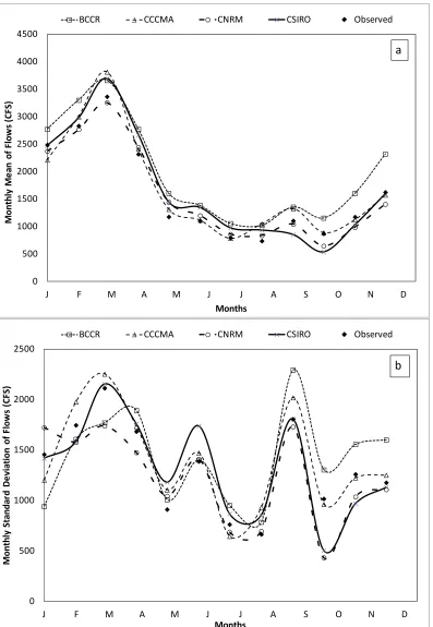
wetter conditions during the winter, whereas the spring flows indicate increased wetter conditions along with pronounced variability in net-inflows. These two projected changes could significantly impact the operation of the reservoir, since the within-year system is expected to refill by April 1 for ensuring the summer demand. Comparing the average monthly releases above 625 CFS over the period 1981-2010 (2324 CFS) with the projected average monthly releases from GCMs (BCCR: 2565 CFS, CCCMA: 2405 CFS, CNRM: 2247 CFS, CSIRO: 2440 CFS), all models indicate an increased scenario of net-inflows into the Lake, which could in general result in an increased downstream releases (> 625 CFS) to ensure the current operational pool level of 216 ft-MSL. Since the projected increases in water demand would result in tapping more water from the conservation storage (202 ft to 216 ft-MSL), this may result in demand-induced droughts since the operational rule curves maintaining 216 ft-MSL. The next section evaluates different scenarios of increased demand for improving the operation of Lake Jordan reservoir system utilizing the generated net-inflows obtained from near-term climate change projections.
4 Results and Analyses
The proposed study focuses on water management of the within-year system, Lake Jordan, over the next 10-30 years based on the projected changes in net-inflows arising from near-term climate change by: 1) quantifying the uncertainty in meeting the current allocation/demand for water supply, water quality and flood control (Scenario 1: climate change impact alone with no increase in demand); 2) analyzing the impact of increased water supply demand on delivering the desired reliabilities on water supply, downstream water quality protection and flood control based on the existing operational policies as specified by the rule curves (Scenario 2: climate change impacts under increased demand with no reallocation strategies) and 3) identifying the revised operational policies for ensuring current reliabilities on water supply, water quality and flood protection even under increased water supply demand (Scenario 3: climate change impacts under increased demand by considering reallocation). To address the first scenario, we first obtained changes in the mean monthly inflows over the next 30 years by forcing downscaled near-term climate change projections from four different GCMS (Maurer et al. 2007) on the calibrated SWAT model for the upper Cape Fear River basin. The SWAT predicted inflows over the period 2012-2041 were then input into the Jordan Lake reservoir model under current reservoir operation policy with no anticipated increase in water demand. Under Scenario 2, the performance of current operational policies was analyzed with increased water supply demand with the same inflows obtained from the SWAT model. Finally, under Scenario 3, the analyses focused on identifying revised allocation strategies that ensure current risk-levels for flood control, water supply delivery and water quality protection under near-term climate change and increased water supply demand.
12
release is zero, which indicates a severe drought condition. For surplus release risk, we first estimate the number of months in which the monthly release is greater than the required release (625 CFS), which indicates additional release to adhere to the operational rule curve of 216 ft-MSL. Following that, we also quantify extreme flood risk based on the number of months in which the monthly release exceeds the allowed flood release of 5000 CFS. Both the flood/surplus and drought risk attributes for the baseline period as well as each GCM under the near-term climate change period are expressed as a probabilities based on the total number of event occurrences to the total months over the period of analyses (240 months). Apart from the probabilities, we also quantify the average and standard deviation of monthly releases if the adjusted releases in a given month are above/below 600 CFS. Similar information is also provided if the monthly releases are above 5000 CFS.
4.1 Baseline Flood and Drought Risks
Under current operational management, the required release is set to 625 cubic feet per second (CFS) including 600 CFS for water quality and 25 CFS for water supply. Table 2 provides the baseline estimates of current flood/surplus and drought risks under existing operational policies. Based on this, the probability of meeting required releases of 625 CFS is about 66% while the probability of flood releases, i.e. releases greater than 5000 CFS, is 4.7%. These two attributes quantify the current flood/surplus risk at the Jordan Lake. Looking at the drought risks, the probability when model release is less than the required release of 625 CFS is 2%. This indicates that reservoir released the exact release of 625 CFS in 32% of months. We also noted that there is only 0.5% probability when monthly releases are zero. Although the drought risk seems to be small under existing demand, it could change significantly under near-term climate change in meeting the existing demand. We evaluate this scenario next.
4.2 Flood/Surplus and Drought Risks under Near-term Climate Change (Scenario 1)
13
almost three models except the CNRM model indicate increased flood risk with more months having greater than 5000 CFS. This is also further confirmed with the increase in fraction of months with average releases above 5000 CFS by the above three models.
To understand which months/seasons experience pronounced changes with releases greater (lesser) than 625 CFS, we show the seasonality of release patterns in Figure 5a (Figure 5b). It is clear that the winter and spring months experience a more pronounced increase in releases > 625 CFS (Figure 5a), whereas releases lesser than 625 CFS are experienced more in the spring and summer months (April to August). The surplus releases (release greater than 625 CFS) are also more pronounced in the winter and spring months. Thus, the overall increase in net-inflows seems to increase flood risk and more variability in allocation.
4.3 Flood and Drought Risks with Increased Water Demand (Scenario 2)
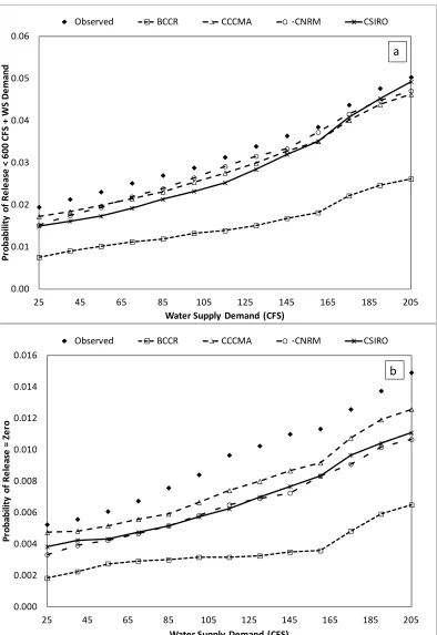
Given that the water supply demand in the Triangle (Raleigh-Durham-Chapel Hill) area have grown up by 20%-60% during 1995-2000 (Weaver, 2005), we assumed a moderate 30% increase in water supply demand for the Triangle area as well as for the downstream cities (Fayetteville and Wilmington) for every five year over the period 2012 to 2041. This implies that the water supply demand of 25 CFS in 2012 could increase up to 205 CFS by 2041. This water supply release needs to be met along with the required downstream water quality protection release of 600 CFS. The reservoir model is evaluated with the generated net-inflows using the observed monthly statistics over the period 1991-2010 and using the projected monthly statistics over the period 2012-2041. Figure 6 shows the probability of surplus releases (probability of flood release > 5000 CFS) as a function of different target releases. With increased water supply demands, all GCMs show a clear decrease in probability of surplus releases (Figure 6a). This is natural to expect since increased demand will stress the conservation storage more resulting in decreased surplus releases. This decline is present across all GCMs with a decrease of about 8.3% (20 months out of 240 months) in which the model-suggested releases exceed the required release. Further, from Figure 6a, BCCR is the only GCM that stands out from the other models due to its relatively wetter projections of near–term climate change. In contrast, there is no significant decline in the months with release at the maximum flood level (Figure 6b).
As expected, all GCMs suggest increase in drought risk on both attributes – the probability of deficit in meeting the target releases (Figure 7a) and the probability of zero release under increased water supply demand (Figure 7b) – as the water supply demand increases. For comparison, we also provide the estimated drought risk under current inflow conditions which do not consider projected climate change. Since the net-inflows are expected to increase under climate change, for a given water supply demand, the drought risk estimated by the net-inflows decrease in comparison to the drought risk for the current inflow conditions. Most of the shortfalls typically occur in the summer and fall months, since the projected net-inflows are lower during those months. The change in the seasonality in shortfalls remains the same between the observed and the projected inflows. In the next section, we evaluate whether we can offset the increased drought risk due to climate change and projected population growth by altering operational strategies.
4.4 Intervention: Reallocation of Existing Storages (Scenario 3)
14
drought risk is to increase the conservation storage in the reservoir so that the resulting risk remains the same as that of current risk for the desired yield of 625 CFS. However, this increased water supply allocation should not result in any increased downstream extreme flood risk (i.e., probability of release = 5000 CFS). Similarly, increasing the water supply allocation alone is bound to increase the probability of shortfalls on water quality releases (600 CFS) for a given set of net-inflows if the operating rule curve is fixed. Hence, we ensure that both the probability of extreme flood risk (5000 CFS) and the probability of shortfalls on water supply and water quality releases (600 CFS) remain as that of current risk reported in Table 2 for a given set of inflows. Since changing the rule curve from 216 ft-MSL to 220 ft-MSL did not change the probability of no release under observed flows as well as under GCM projected net-inflows, we dropped that criterion from the analyses. Further, the probability of surplus releases beyond water supply and water quality releases is naturally expected to go down by increasing the operational rule curve, since the reservoir can hold additional water as conservation storage. Hence, that metric is also not considered here. The goal here is to find increased water supply releases (Table 3) that is permissible under various operating levels such that the extreme flood risk and the probability of shortfalls on increased water supply and water quality releases remain as that of current risk (Table 2) for a given set of net-inflows.
Table 3 provides the permissible water supply releases under different operating levels (ranging from 216 ft-MSL to 220 ft-MSL) for both observed net-inflows (i.e., no climate change impacts) as well as under GCM-projected net-inflows for the period 2012-2041. Under observed inflow pattern which assumes no climate change impacts, the existing operating rule curve at 216 ft-MSL has to be increased for potential water supply allocation due to future population growth demands particularly to ensure that the probability of shortfalls on water supply and water quality releases remain at the current risk level (0.020) in Table 2. Information in Table 3 could also be employed for adaptive planning depending on the level of population growth in the area. Thus, as the population grows in the Triangle area, water managers could potentially change the rule curve that ensures the current level of probability of shortfalls and flood risk. Based on this, we infer that by increasing the rule curve to 220 ft-MSL, a total of 190 CFS could be allocated to water supply release for ensuring current flood and drought risks.
15
5. Discussion
The main objective of this study is to quantify the impacts of near-term climate change and increased water demand on a within-year reservoir system, Jordan Lake, which supplies water to the Triangle Area in NC. By forcing the SWAT model with downscaled inputs from four selected GCMs under the A1B climate change scenario (Maurer et al. 2007), we obtained the change in the mean monthly inflows and standard deviation of the monthly inflows between the baseline period (1981-2010) and the planning period (2012-2041). These differences in the mean monthly net-inflows and the standard deviation in the net-inflows were then added to the USACE’s observed net-inflows for the period 1981-2010 to obtain the projected net-inflows for the period 2012-2041. These projected mean monthly net-inflows and variances of the monthly net-inflows for each GCM were combined by preserving month-to-month correlations to generate 50 sets/realizations of monthly inflows over the period 2012-2041 for further analyses in understanding the impact of climate change and urbanization on the Lake Jordan within-year reservoir system.
The primary advantage in using the stochastic generation scheme for obtaining the net-inflows is in developing multiple realizations based on the expected changes in mean and variance in monthly streamflows. On the other hand, if we were to use the bias-corrected net-inflows obtained from SWAT model, then we would have had just only one realization of monthly inflows for the period 2012-2041. Since these climate models were initialized with initial atmosphere and ocean conditions based on 20th century control simulations, the primary information from these GCMs lies in their ability in predicting mean monthly values and variances of the monthly values rather than in predicting monthly time series of precipitation and temperature obtained from these GCMs. Hence, we combined the changes in the mean monthly net-inflows and variances in the monthly net-inflows with a parametric streamflow generation model for obtaining multiple realizations of net-inflows for the reservoir analyses.
One allied goal of this paper is to offer additional insights on the behavior of within-year reservoir system under near-term climate change. Within-year (over-year) reservoir systems are more common in the humid (arid) eastern (western) US due to the smaller (larger) interannual variability in streamflows. For this purpose, we consider the resilience index, m, of a reservoir system (Vogel and Stedinger (1987) and Vogel and Bolognese (1995)):
Cv
m=(1−α)/ …(12)
16
Figure 8 shows the failure probability of releases as a function of system resilience for both observed inflows and GCM-projected inflows under two different operating levels of 216 ft (8a) and 220 ft above MSL (8b). For a given set of inflows, as the water supply demand increases from 25 CFS to 205 CFS, the failure probability increases. However, with the exception of BCCR model, the failure probability obtained based on observed inflows and the rest of the three GCM-projected inflows do not differ much over the increased demand of 25 CFS to 205 CFS. Since BCCR estimates high mean annual inflows, its failure probability is much lower than the rest of the flow scenarios. Perhaps the most important information from Figure 8 is the variability in the system resilience (m). Each value of m corresponds to the total yield (water quality release + increased water supply release) from the system for a given coefficient of variation of flow estimated by the inflow scenario. Thus, resilience is a function of both inflow characteristics as well as the total yield expected from the system. Even though the failure probability of yield remains the same between the observed inflows (i.e., no climate change impacts) and the GCM-projected inflows, the impact of climate change is more on reservoir resilience. Relatively smaller change in the failure probability across the inflows is due to the ability to supply water purely from the initial storage. This is consistent with the findings of Letttenmaier et al. (1999) over few selected reservoirs in the eastern US. But, the primary impact of climate change is on reducing the resiliency of within-year reservoir systems which forces the system behavior to be a more over-year system.
Thus, due to climate change, reservoir systems will take more time to recover as both the coefficient of variation of projected inflows and the fractional yield, α, increase. The observed coefficient of variation (CV) of annual streamflows ranges between 0.2-0.4 for the eastern US with smaller CV being observed over the Northeast and higher CV being observed in the temperate Southeast (Vogel et al. 1998). Recent studies on the impact of climate change on the eastern US has suggested increase in the coefficient of variation of runoff over the southeastern US by 1.5 to 2 times (Milly et al. 2005; Hayhoe et al. 2006; Lettenmaier et al. 2008) though considerable differences lie across the models. Our findings are consistent with the above studies suggesting increased winter flows and reduced summer flows resulting in overall increased coefficient of variation of annual flows. Depending on the magnitude of the changes in CV of annual flows, the behavior of the within-year reservoir system could approach towards that of over-year reservoir system which could result in reduced resiliency of the system. Our future effort will focus on quantifying the changes in the coefficient of variation of annual flows based on the recent generation AR5 climate model runs.
6. Concluding Remarks
17
and the standard deviation of the monthly inflows under climate change. By generating the inflows using the stochastic streamflow generation model, we forced the reservoir model with multiple realizations of streamflow traces that preserve the projected changes in monthly streamflow statistics.
Our results indicate that under near-term climate change alone with no increase in water supply demand in a within-year reservoir system, Lake Jordan, there is no consistent trend in the probability of surplus releases (> 625 CFS) by the four GCM’s considered in this study while there is a decrease in shortfall releases (< 625 CFS) due to increase in net-inflows during winter and spring months. Under both climate change and projected water supply demand over 2012-2041, drought risk (probability of releases < 600 CFS + water supply demand and probability of zero releases) increases while there is a decrease in risk associated with surplus releases (> 600 CFS + water supply demand). This is expected since increase in water demands will stress the conservation storage. In particular, there is no significant decrease in maximum flood release of greater than 5000 CFS. Under near-term climate change, increase in water supply demands from 25 CFS up to 205 CFS can be offset by increasing the rule curve from 216 MSL to 220 ft-MSL without changing the observed flood and drought risks under existing operations.
18
7. References
Anderson J, Chung F, Anderson M, Brekke L, Easton D, Ejeta M, Peterson R, Snyder R (2008) Progress on Incorporating Climate Change Into Management of California’s Water Resources. Climatic Change 87:S91-S108.
Arnold JG, Srinivasan R, Muttiah RS, Williams JR (1998), Large Area Hydrologic Modeling and Assessment Part I: Model Development. Journal of the American Water Resources
Association, 34(1): 73-89.
Boyles R, Raman S (2003) Analysis of climate trends in North Carolina (1949-1998). Environment International, 29, 263-275.
L. Brekke, Kiang JE, Olsen JR, Pulwarty RS, Raff DA, Turnipseed DP, Webb RS, White KD (2009) Climate change and water resources management—A federal perspective: U.S.
Geological Survey Circular 1331, 65 p. (http://pubs.usgs.gov/circ/1331/.)
Christensen NS, Wood AW, Voisin N, Lettenmaier DP, Palmer RN (2004) The Effects of Climate Change on the Hydrology and Water Resources of the Colorado River Basin. Climatic Change 62:337-363.
Christensen JH, et al. (2007) Regional climate projections. In: Solomon, S., et al. (Eds.), Climate Change 2007: The Physical Science Basis. Contribution of Working Group I to the Fourth Assessment Report of the Intergovernmental Panel on Climate Change. Cambridge University Press, Cambridge, United Kingdom and New York, NY, USA.
Déqué M, Dreveton C, Braun A, Cariolle D (1994) The ARPEGE/IFS atmosphere model : A contribution to the French community climate modelling. Climate Dyn., 10, 249-266.
Déqué M, Piedelievre JP (1995) High resolution climate simulation over Europe. Climate Dyn., 11, 321-339.
Flato, GM, Boer GJ, Lee WG, McFarlane NA, Ramsden D, Reader MC, Weaver AJ (2000) "The Canadian Centre for Climate Modeling and Analysis global coupled model and its climate". Climate Dynamics 16 (6): 451–467. doi:10.1007/s003820050339
Gangopadhyay S, Clark M, Rajagopalan B (2005) Statistical downscaling using K-nearest neighbors. Water Resour. Res., 41, W02024, doi:10.1029/2004WR003444.
Gleick PH (1987) Regional hydrologic consequences of increases in atmospheric carbon dioxide and other trace gases. Climatic Change 10(2), 137–161.
Gleick PH, Chalecki EL (1999) The impact of climatic changes for water resources of the Colorado and Sacramento-San Joaquin river systems. Journal of the American Water Resources Association 35(6), 1429–1441.
Golembesky K, Sankarasubramanian A, Devineni N (2009) Improved Drought Management of Falls Lake Reservoir: Role of Multimodel Streamflow Forecasts in Setting up Restrictions. Journal of Water Resources Planning and Management,135(3), 188-197, 2009.
Gordon HB, Rotstayn LD, McGregor JL, Dix MR, Kowalczyk EA, O'Farrell SP, Waterman LJ, Hirst AC, Wilson SG, Collier MA, Watterson IG, Elliott TI (2002) The CSIRO Mk3 Climate System Model [Electronic publication]. Aspendale: CSIRO Atmospheric Research. (CSIRO Atmospheric Research technical paper; no. 60). 130 pp.
19
Hanak E, Lund J (2012) Adapting California’s Water Management to Climate Change. Climatic Change 111:17–44.
Hawkins E, Sutton R (2009) The potential to narrow uncertainty in regional climate predictions. Bull. Amer. Meteor. Soc., 90, 1095–1107.
Hayhoe K, Wake C, Huntington TG, Luo L, Schwartz MD, Sheffield J, Wood EF, Anderson B, Bradbury J, DeGaetano TT, Wolfe D (2006) Past and future changes in climate and
hydrological indicators in the U.S. Northeast. Climate Dynamics, 10, doi:1007/s00382-006-0187-8.
Hayhoe K, Wake C, Huntington TG, Luo L, Schwartz MD, Sheffield J, Wood EF, Anderson B, Bradbury J, DeGaetano TT, Wolfe D (2007) Past and future changes in climate and
hydrological indicators in the U.S. Northeast. Climate Dynamics 28: 381-407.
Keenlyside NS, Latif M, Jungclaus J, Kornblueh L, Roeckner E (2008) Advancing decadal-scale climate prediction in the North Atlantic sector. Nature 2008; 453: 84-88.
Kyriakidis PC, Miller NL, Kim J (2001) Uncertainty propagation of regional climate model precipitation forecasts to hydrologic impact assessment. Journal of Hydrometeorology, 2, 140-160.
Lettenmaier DP, Brettman KL, Vail LW, Yabusaki SB, Scott MJ (1992) Sensitivity of
Pacific Northwest Water Resources to Global Warming. Northwest Environmental Journal 8 (2), 265–283.
Lettenmaier DP, Wood AW, Palmer RN, Wood EF, Stakhiv EZ (1999) Water resources implications of global warming: A US regional perspective. Climate Change, 43, 537–579.
Lettenmaier DP, Major D, Poff L, Running S (2008) Water Resources. In: The effects of climate change on agriculture, land resources, water resources, and biodiversity in the United States. A Report by the U.S. Climate Change Science Program, and the Subcommittee on Global Change Research. Washington, DC., USA, 362 pp
Lyon B, Christie-Blick N, Gluzberg Y (2005) Water shortages,development, and drought in Rockland County, New York. J. Am. Water. Res. Assoc., 41(6), 1457-1469.
Maurer EP, Wood AW, Adam JC, Lettenmaier DP, Nijssen B (2002) A long-term
hydrologically based dataset of land surface fluxes and states for the conterminous Unites States. Journal of Climate, 15, 3237-3251.
Maurer EP, Brekke L, Pruitt T, Duffy PB (2007) Fine-resolution climate projections enhance regional climate change impact studies. Eos Trans. AGU, 88(47), 504
McCabe GJ, Wolock DM (1999) General-circulation-model simulations of future snowpack in the western United States. Journal of the American Water Resources Association, v. 35, p. 1473-1484.
20
Milly PCD, Dunne KA, Vecchia AV (2005) Global pattern of trends in streamflow and water availability in a changing climate. Nature 438: 347-350
Milly PCD, Betancourt J, Falkenmark M, Hirsch RM, Kundzewicz ZW, Lettenmaier DP, Stouffer RJ (2008) CLIMATE CHANGE: Stationarity Is Dead: Whither Water Management? Science 319:573-574.
Moreau DH (2006) North Carolina’s Abundant Water Resources: Supply, Use and Imbalances, WRRI News Letter, 355, May-June 2006.
Nakicenovic N et al. (2000) Special Report on Emissions Scenarios: A Special Report of Working Group III of the Intergovernmental Panel on Climate Change, Cambridge University Press, Cambridge, U.K., 599 pp. Available online
at: http://www.grida.no/climate/ipcc/emission/index.htm
North Carolina Drought Management Advisory Council, http://www.ncdrought.org/ North Carolina State Climate Office, http://www.nc-climate.ncsu.edu/
Petersen T, Devineni N, Sankarasubramanian A (2012) Seasonality of Monthly Runoff over the Continental United States: Causality and Relations to Mean Annual and Mean Monthly Distributions of Moisture and Energy. Journal of Hydrology,468-469 ,pp.139-150.
Prairie J, Rajagopalan B, Lall U, Fulp T (2007) A stochastic nonparametric technique for space-time disaggregation of streamflows. Water Resources Research, 43, W03432, 1-10, doi:10.1029/2005WR004721.
Rajagopalan B, Nowak K, Prairie J, Hoerling M, Harding B, Barsugli J, Ray A, Udall B (2009) Water supply risk on the Colorado River: Can management mitigate? Water Resour. Res., 45, W08201, doi:10.1029/2008WR007652.
Royer JF, Cariolle D, Chauvin F, Déqué M, Douville H, Hu RM, Planton S, Rascol A, Ricard JL, Salas y Mélia D, Sevault F, Simon P, Somot S, Tytéca S, Terray L, Valcke S (2002)
Simulation des changements climatiques au cours du 21-ième siècle incluant l'ozone stratosphérique. C. R. Geophys., 334, 147-154.
Sankarasubramanian A, Vogel RM (2002) Comment on the paper: Basin hydrologic response relations to distributed physiographic descriptors and climate, Journal of Hydrology,263,257-261.
Sankarasubramanian A, Vogel RM (2003) Hydroclimatology of the continental U.S. Geophysical Research Letters,30(7), art.no.1363.
Schnoor JL (2012) The U.S. Drought of 2012. Environ. Sci.Technol. 46(19):10480-10480. Sinha T, Cherkauer KA (2010) Impacts of future climate change on soil frost in the
Midwestern United States. J. Geophys. Res., 115, D08105, 1-16.
Smith DM, Cusack S, Colman AW, Folland CK, Harris GR, Murphy JM (2007) Improved surface temperature prediction for the coming decade from a global climate model. Science, 317, 796–799, doi:10.1126/science.1139540.
21
Stone MC, Hotchkiss RH, Hubbard CM, Fontaine TA, Mearns LO, Arnold JG (2001) Impacts of climate change on Missouri River Basin watershed yield. Journal of the American Water Resources Association, 37(5), 1119-1129.
Vicuna S, Dracup JA, Lund JR, Dale LL, Maurer EP (2010) Basin-Scale Water System Operations With Uncertain Future Climate Conditions: Methodology and Case Studies. Water Resources Research 46:W04505, doi: 10.1029/2009 WR007838.
Vogel RM and Stedinger JR (1987) Generalized storage-reliability-yield relationships. J. Hydrol., 89: 303-327.
Vogel RM, Bolognese RA (1995) Storage-reliability-resiliency-yield relations for over-year water supply system, Water Resour. Res. 31(3), 645-654.
Vogel RM, Tsai Y, Limbrunner JF (1998) The regional persistence and variability of annual streamflow in the United States, Water Resour. Res., 34(12), 3445–3459.
Vogel RM, Lane M, Ravindiran RS, Kirshen P (1999) Storage Reservoir Behavior in the United States, Journal of Water Resources Planning and Management, ASCE, 125(5), Sep/Oct, 1999.
Weaver CJ (2005) The drought of 1998–2002 in North Carolina–Precipitation and hydrologic conditions. USGS Scientific Investigations Rep., Washington, D.C.
U.S. Census Bureau (2009) Population Division, http://www.census.gov/popest/housing/HU-EST2009-top100.html
22
8 Tables
Table 1: Performance of SWAT model in simulating the flows at Haw River near Bynum using observed (1/8 degree) and projected climate forcings from four different GCMs during 1981-2010.
Climate Forcings
Streamflow Statistics Observed BCCR CCCMA CNRM CSIRO
Absolute Percentage Bias 27.7 70.3 70.4 72.2 70.2
Simulated Mean (CFS) 1410 1204 1204 1204 1204
Coefficient of variation simulated 0.78 0.67 0.72 0.76 0.74
Root Mean Square Error 36.3 96.2 97.3 100.6 98.8
Correlation Coefficient 0.94 0.32 0.33 0.31 0.32
USACE’s Observed Mean (CFS) 1204 - - - -
23
Table 2: Baseline flood/surplus and drought risks for Jordan Lake based on observed net-inflows and inflows generated based on the projected precipitation from different GCMs in meeting water quality (600 CFS) and water supply (25 CFS) demands. The probability of flood risk is assessed based on monthly releases above 5000 CFS. Entries in the last three rows of the table have units of CFS, and represent increments below (second to last row) or above (last and third to last rows) 625 or 5000 CFS, e.g., for months with releases >5000 CFS, the BCCR model gave an average monthly release of 1324 CFS in excess of 5000 CFS (i.e., an average monthly release of 5000 + 1324 = 6324 CFS).
Flood and Drought Attributes
Stochastic Generation Model
Observed BCCR CCCMA CNRM CSIRO
Fraction of months with release >625 CFS 0.658 0.745 0.669 0.648 0.648
Fraction of months with release < 625 CFS 0.02 0.008 0.017 0.015 0.015
Fraction of months with no release 0.005 0.002 0.005 0.003 0.004
Fraction of months with release > 5000 CFS 0.047 0.063 0.063 0.035 0.06
Average monthly release (CFS) in excess of 625 CFS 2324 2565 2405 2247 2440
Average monthly release (CFS) in shortfall of 625 CFS 264 294 295 327 326
24
Table 3: Increased water supply releases (in cfs) under different operating levels for observed flows and GCM-projected net-inflows over the planning period 2012-2041.
Elevation (ft)
Observed (cfs)
BCCR (cfs)
CCCMA (cfs)
CNRM (cfs)
CSIRO (cfs)
216 25 165 55 55 75
217 70 205 100 85 115
218 115 205 130 130 150
219 160 205 165 175 190
25
9 Figures
Figure 1: Location of Jordan Lake Reservoir in the Upper Cape Fear River Basin. The shaded areas indicate the four counties (Wake, Orange, Durham and Chatham) that are experiencing tremendous growth in population.
Wake Durham
Orange
26
Figure 2: Schematic diagram for evaluating the impacts of near-term climate change and increased water supply demand on the Jordan Lake Reservoir
GCM Gridded Climate Data from 1981-2010 (Maurer et al. 2007)
GCM Gridded Climate Data from 2012-2041 (Maurer et al. 2007)
SWAT Model Soil Data (STATSGO)
Land Cover Data (NLCD 2001)
Temporal Downscaling K-NN Method (Prairie et al. 2007)
Monthly Inflows from 1981-2041
Add the Observed Mean Monthly and Variance from the Period 1981-2010
Future Water Demand
Jordan Lake Reservoir Model
Assess Impacts of Near-Term Climate Change on
Water Availability Changes in Mean Monthly Inflows and Variance between Two
27
Figure 3: Pertinent data relevant to Jordan Lake Reservoir
202 MSL 216 MSL
261 MSL
240 MSL
Uncontrolled Flood Storage
Controlled Flood Storage
Conservation Storage
600 CFS Water Quality and 25 CFS Water Supply Release 5000 CFS Max Flood Release
28
Figure 4: (a) Mean monthly streamflow and (b) standard deviation of monthly streamflows for the observed period 1981-2010 and the future period 2012-2041 based on four different GCMs.
0 500 1000 1500 2000 2500 3000 3500 4000 4500
J F M A M J J A S O N D
M ont hl y M ea n of F lo w s ( CF S) Months
BCCR CCCMA CNRM CSIRO Observed
a 0 500 1000 1500 2000 2500
J F M A M J J A S O N D
M ont hl y S ta nda rd De vi at io n of F lo w s ( CF S) Months
BCCR CCCMA CNRM CSIRO Observed
29
Figure 5: Number of months with water supply and water quality releases (a) greater than the target releases and b) less than the target releases over the observed period (1981-2010) and the projected period 2012-2041 (four GCMs). Water quality releases and water supply releases are assumed as 600 CFS and 25 CFS based on the current
operational rule curve of 216 MSL level.
0 2 4 6 8 10 12 14 16 18 20
J F M A M J J A S O N D
N um be r o f M ont hs w ith Re le as e > 6 00 C FS + W S D em and Months
BCCR CCCMA CNRM CSIRO Observed
a 0 0.5 1 1.5 2 2.5 3
J F M A M J J A S O N D
N um be r o f M ont hs w ith Re le as e < 6 00 C FS + W S D em and Months
BCCR CCCMA CNRM CSIRO Observed
30
Figure 6: Impacts on flood/surplus risk under near-term climate change and increased water supply demand for the existing operating rules with (a) probability of exceeding the projected required water supply release and target water quality release and (b) probability of occurrence of maximum allowed flood release.
0.50 0.55 0.60 0.65 0.70 0.75 0.80
25 45 65 85 105 125 145 165 185 205
Pr ob ab ili ty o f R el ea se > 600 CFS + W S D em an d
Water Supply Demand (CFS)
Observed BCCR CCCMA CNRM CSIRO
a 0.02 0.03 0.04 0.05 0.06 0.07
25 45 65 85 105 125 145 165 185 205
Pr ob ab ili ty o f R el ea se = F lo od R el ea se
Water Supply Demand (CFS)
Observed BCCR CCCMA CNRM CSIRO
31
Figure 7: Impacts on drought risk under near-term climate change and increased water supply demand for the existing operating rules with (a) failure probability in meeting the projected required water supply release and the target water quality release and (b) probability of occurrence of no releases for both water supply and water quality uses. 0.00 0.01 0.02 0.03 0.04 0.05 0.06
25 45 65 85 105 125 145 165 185 205
Pr ob ab ili ty o f R el ea se < 600 CFS + W S D em an d
Water Supply Demand (CFS)
Observed BCCR CCCMA CNRM CSIRO
a 0.000 0.002 0.004 0.006 0.008 0.010 0.012 0.014 0.016
25 45 65 85 105 125 145 165 185 205
Pr ob ab ili ty o f R el ea se = Z er o
Water Supply Demand (CFS)
Observed BCCR CCCMA CNRM CSIRO
32
Figure 8: Relationship between failure probability of target releases (water supply and water quality) and reservoir resilience under climate change and urbanization under operating rule - curve (a) 216 ft-MSL and (b) 220 ft-MSL.
0.00 0.01 0.02 0.03 0.04 0.05 0.06
0.8 1.0 1.2 1.4 1.6 1.8
Fa ilu re P ro ba bi lit y o
f T
ar
ge
t R
el
ea
se
s
Resilience Index, m
Operating Level - 216
Obs BCCR CCCMA CNRM CSIRO a
0.00 0.01 0.01 0.02 0.02 0.03
0.8 1.0 1.2 1.4 1.6 1.8
Fa ilu re P ro ba bi lit y o
f T
ar
ge
t R
el
ea
se
s
Resilience Index, m
Operating Level - 220