Numerical Study of a System of Long Josephson Junctions with
Inductive and Capacitive Couplings
I. R. Rahmonov1,2,a, Yu. M. Shukrinov1,3,b, A. Plecenik4,c, E. V. Zemlyanaya3,5,d, and M. V. Bashashin3,5,e
1BLTP, Joint Institute for Nuclear Research, 141980 Dubna, Russia 2Umarov Physical and Technical Institute, Dushanbe, Tajikistan
3Dubna International University for Nature, Society and Man, Dubna, Russia 4Department of Experimental Physics, Comenius University, Bratislava, Slovakia 5LIT, Joint Institute for Nuclear Research, 141980 Dubna, Russia
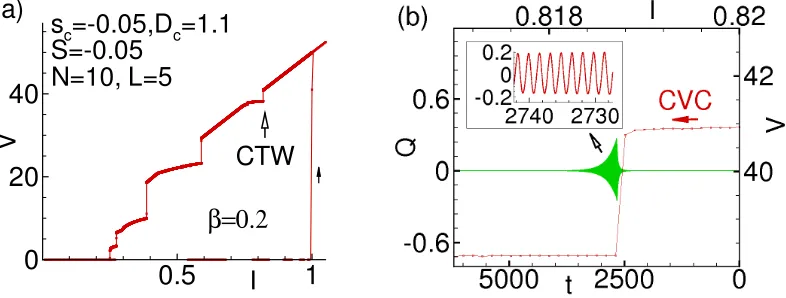
Abstract.The phase dynamics of the stacked long Josephson junctions is investigated taking into account the inductive and capacitive couplings between junctions and the diffusion current. The simulation of the current–voltage characteristics is based on the numerical solution of a system of nonlinear partial differential equations by a fourth order Runge–Kutta method and finite-difference approximation. A parallel implementation is based on the MPI technique. The effectiveness of the MPI/C++code is confirmed by calculations on the multi-processor cluster CICC (LIT JINR, Dubna). We demonstrate the appearance of the charge traveling wave (CTW) at the boundary of the zero field step. Based on this fact, we conclude that the CTW and the fluxons coexist.
1 Introduction
The layered high-temperature superconducting materials such as Bi2Sr2CaCu2O8+δ(BSCCO) can be considered as a stack of coupled intrinsic Josephson junctions (JJ) [1]. This system is one of the promising objects of superconducting electronics [2, 3]. Coherent terahertz electromagnetic radiation from this system provides wide possibilities for various applications [4]. However, the mechanism of this radiation is still unclear. The most intense coherent radiation corresponds to the region of the current–voltage characteristic (CVC) where switching from the upper branch to inner branches occurs [3]. In this region of the CVC the Josephson oscillations excite a longitudinal plasma wave due to the parametric resonance [5]. In stacked long Josephson junctions (SLJJ) with the lengthL larger than the Josephson penetration depthλJ(L> λJ) the parametric resonance can be realized in the zero field step region [6, 7] of the CVC and the fluxons coexist with the longitudinal plasma wave, which can be interpreted as the collective excitation [8]. Other types of the collective states [9] in the stack of coupled JJs are the Josephson plasma [10] and the charge traveling wave (CTW) [11] along
ae-mail: [email protected],[email protected] be-mail: [email protected]
ce-mail: [email protected] de-mail: [email protected]
ee-mail: [email protected]
C
the stack. A stack of coupled JJs can be considered as a laboratory for the study of the collective excitations in superconducting nanostructures. First of all, the investigation of the long JJs stack is an actual problem, because most of the experimental results were obtained for this system. Therefore, the construction of a model that ensures an adequate description of the properties of the SLJJ in the high temperature superconductors is one of the topical tasks of the modern physics of the superconductivity and, also, an actual problem is the construction of effective numerical algorithms for the simulation of the phase dynamics of the SLJJ.
To describe the SLJJ, Sakai, Bodin, and Pedersen [12] proposed a model taking into account the inductive coupling between JJs. Machida and Sakai [13] proposed a generalization of the model to the case of both inductive and capacitive coupling. However, they disregarded the diffusion current [14], the significance of which was emphasized in [15]. Furthermore, the CVC have not yet been studied within the generalized Machida–Sakai model.
In this paper, we investigate the phase dynamics of the SLJJ taking into account the inductive and capacitive couplings [12, 13] and the diffusion current [15]. Simulation is based on a numerical solution of a system of nonlinear partial differential equations by a fourth order Runge–Kutta method, finite-difference approximation, and the MPI technique for parallel implementation. The effectiveness of the MPI/C++code is confirmed by calculations on the multi-processor cluster CICC (LIT JINR, Dubna).
2 Theoretical model and numerical approach
We use the model with inductive and capacitive couplings [12, 13] and with the diffusion current [15]. The SLJJ has a layered structure withN+1 superconducting and interjacent insulating layers. The x-axis is directed along the length L, they-axis along the width of the superconducting layers and thez-axis is perpendicular to the superconducting layers. Each superconducting layer is described by the Ginzburg–Landau order parameterΔl=|Δ0|exp (iθl). Thel-th and the (l−1)-th superconducting layers form thel-th JJ and it is described by the gauge–invariant phase difference (1) of the Ginsburg– Landau order parameter [13]
ϕl=θl−θl−1−2e
c zl
zl−1
Azdz, (1)
whereθlis the phase of the order parameter of thel-th superconducting layer,eis the electrical charge,
is the Plank constant,cis the speed of the light in vacuum andAzis the vector potential. The system of equations which describes the phase dynamics of the coupled long JJs stack in terms of normalized quantities can be written as follows:
⎧⎪⎪⎪ ⎪⎪⎪⎪⎨ ⎪⎪⎪⎪⎪ ⎪⎪⎩
∂ϕl
∂t =DCVl+sCVl+1+sCVl−1,
∂Vl
∂t = N
k=1
£−lk1∂
2ϕ
k
∂x2 −sinϕl+β ∂ϕl
∂t +I,
(2)
whereDC =1+(2λe/dI) coth(ds/λe),λe-the Debye screening length,dI anddsdenote the thickness of the insulating and the superconducting layers,sC=−λe/[dIsinh(ds/λe)] is the capacitive coupling parameter,Vlis the voltage of thel-th JJ normalized toV0 =ωp/(2e),ωp =
£= ⎛ ⎜⎜⎜⎜⎜ ⎜⎜⎜⎜⎜ ⎜⎜⎜⎜⎜ ⎜⎜⎜⎜⎜ ⎜⎜⎜⎜⎜ ⎜⎝
1 S 0 . . . S
S 1 S 0 . . .
0 S 1 S 0 . . .
... ... ... ... ... ... ... ...
. . . 0 S 1 S
S . . . 0 S 1
⎞ ⎟⎟⎟⎟⎟ ⎟⎟⎟⎟⎟ ⎟⎟⎟⎟⎟ ⎟⎟⎟⎟⎟ ⎟⎟⎟⎟⎟ ⎟⎠ ,
whereS = sL/DL,DL =dI+2λLcoth(ds/λL) is the effective magnetic thickness,λLis the London penetration depth andsL=−λL/sinh(ds/λL) is the parameter of the inductive coupling. In the system of equations (2) the time is normalized to the reverseωp and the coordinatex– to the Josephson penetration depthλJ. The initial conditions for the system of equations (2) areϕl(x,0) = 0 and Vl(x,0) = 0. The coordinate derivative of the phase difference at the boundaries is equal to the external magnetic field∂ϕl(0,t)/∂t=∂ϕl(L,t)/∂t=Bext.
The main tasks are to calculate the CVC, the spatio-temporal dependence of the magnetic field in the JJs, and the electric charge in the superconducting layers. First of all, we should solve numerically the system of partial differential equations (2). We introduce the uniform mesh with the stepsizeΔx in the coordinatexalong the JJ and the stepsizeΔt in time. We putΔt = Δx/5 in accordance with the Courant–Friedrichs–Lewy condition in order to provide the stability of the numerical scheme. We denote the discrete coordinate byxi = Δx×(i−1), wherei = 1, . . . ,NxandNx = L/Δx+1 is the number of coordinate nodes. The discrete time is denoted bytj = Δt×j, where j = 0,1,2, . . .Nt. The x = 0 corresponds to x1 and x = L– to xNx. In the same way, t = 0 corresponds tot1 and
t=TmaxtotNt, whereTmaxis the end of the time domain. The standard second order finite difference
approximation in the spatial coordinatexis used,
∂2ϕ1
l
∂x2 =
2(ϕ2l −ϕ1l) Δx2 −
2Bext
Δx ,
∂2ϕi l
∂x2 = ϕi+1
l −2ϕil+ϕi−
1
l Δx2 ,
∂2ϕNx
l
∂x2 =
2(ϕNx−1
l −ϕ
Nx
l )
Δx2 +
2Bext
Δx . The resulting system of ordinary differential equations is solved numerically for a fixed value of the currentIby a 4th-order Runge-Kutta (RK) algorithm (herelis the JJ number) in the interval [0,L] along thex-coordinate and [0,Tmax] in time and obtain theϕl(x,t) andVl(x,t) as functions ofxandt. Next, the obtainedVl(x,t) is averaged with respect to the coordinatexusing
¯ Vl(t)= 1
L
L
0
Vl(x,t)dx (3)
and with respect to the timetusing
Vl= 1 Tmax−Tmin
Tmax
Tmin
¯
Vl(t)dt, (4)
whereTmindenotes the beginning of the averaging interval. The total voltage of the JJs stack can be
calculated usingV = N l=1Vl
. The integrals (3) and (4) are calculated using the Simpson method and the rectangles method, respectively. Then the bias current value is changed byΔIand the above procedure is repeated. In the calculations the bias current increases from the start valueI =0.01 to I=Imaxand then decreases toI=0.
Table 1.Simulation time of CVC in minutes per number of processes
P 1 2 4 6 8 10 12
L=5,N=10 106.2 46.8 27.3 25.7 19.5 14.4 16.7 L=10,N=10 213 92.5 62.5 44.4 42.3 32.4 37.2 L=10,N=3 37.1 19.9 11.3 8.6 7.5 6.4 6.4
to be calculated. In this case, the electric charge, normalized toQ0 =εV0/4πdsdI, is calculated as a
function ofxandtusing the expressionQl(x,t)=Vl(x,t)−Vl−1(x,t) [8]. Then the value ofQl(x,t)
is averaged with respect to the coordinatexusing the Simpson method. For the external current value corresponding to the fluxon states, the magnetic fieldBin the JJs is calculated using the expression Bl= N
k=1
£−1
lk(∂ϕk/∂x). The magnetic field is normalized toB0=c/2eDLλJ.
The parallel algorithm is based on a distribution of the calculations in the coordinate nodes xi between the group ofPmparallel MPI-processes, wherem=0,1. . . ,M. At each time-steptj, each processPmcalculates the RK coefficients andVl(xi,tj),φl(xi,tj) in the nodesimin ≤i <imax, where
imin=m×Lx/Mandimax=(m+1)×Lx/M. At eachtjthe exchange between neighbor processes is
arranged: each processPm(m<M−1) sends the RK coefficients and values ofVandϕati=imax−
1-th point to 1-thePm+1-process; each Pmprocess (m > 0) sends the RK coefficients and solutions at
i=iminto thePm−1-process. In order to calculate the average valueVl, the parallel calculation of the
integral (3) is performed at each time-steptj. EachPm-process calculates the partial sum of elements Vl(xi,tj) at each JJlin accordance to the Simpson quadrature formula. Then the resulting summation is performed in the processP0. In theP0-processVlis averaged in time and in LJJs, and the resulting
value is saved to the file. For some values ofIthe solutionsVl(xi,tj) andφl(ti,tj) are collected in the processP0where they are saved to the file together with the respective physical characteristics.
3 Results and discussions
Let us first of all discuss the effectiveness of the parallel algorithm. The methodical calculations on the CICC multi-processor cluster (LIT JINR) with a different number of parallel MPI-processes are performed. For these calculations we put the number of JJsN =10, the JJ lengthL=5 andL=10; Δx=0.05;ΔI =0.005. Table 1 shows the calculation time (in minutes) of the CVC per number of processes for the stacks withN=3,N=10 JJs and with lengthL=5,L=10. One can see that the developed parallel algorithm provides 6-7 times acceleration (depending on the values ofNandL) as compared to the sequential simulation.
The next step of the parallel optimization of the long JJs stack simulation code is the parallelization of the calculations at each junction.
Let us now discuss the main features of the single long JJ. Figure 1(a) shows the one loop CVC of the single JJ with L = 10. The calculations have been performed for the β = 0.2, Bext = 0,
ΔI=0.0001 andTmax=200. The stepsize in the coordinate and time wereΔx=0.05 andΔt= Δx/5,
respectively. The curve shows the hysteresis and seven step structure at decreasing current. These zero–field steps (ZFS) correspond to the formation of fluxons in the JJs [6, 7]. The velocity of the fluxonuis given by the expression [6, 7]u =[1+4β/πI]−1/2 and it is given in units of the Swihart
I
V
0.5
1
0
2
4
N=1, L=10
B
ext=0,
β=0.2
I=
0.
76
(a)
Figure 1.(a) CVC of the single long JJ withL=10; (b) Spatiotemporal dependence of magnetic field in the JJ atI=0.76
ofnsteps in the CVC [6, 7]. In order to directly demonstrate fluxons, we calculate the spatiotemporal dependence of the magnetic field in JJ. Figure 1(b) shows the time evolution of the spatial distribution of the magnetic field in JJs at the value of current valueI =0.76, which corresponds to the 6th ZFS. It indicates the formation of a state with six fluxons.
I
V
0.5
1
0
20
40
s
c=-0.05,D
c=1.1
S=-0.05
(a)
β=0.2
N=10, L=5
CTW
Figure 2.(a) CVC of stacked long JJs with the lengthL=5; (b) Charge–time dependence in the right boundary of the third ZFS
oscillations increases the charge amplitude, which can be seen in these figures. Since the CTW appears in the CVC region corresponding to the ZFS, we may conclude about the coexistence of the CTW and the fluxons.
4 Conclusions
In this paper, we have investigated numerically the phase dynamics of the SLJJ taking into account the inductive and capacitive couplings between junctions and diffusion current. In our investigation we used the parallel and sequential calculations of CVC. The parallel implementation is based on the MPI technique. We showed that the parallel algorithm results in a seven time acceleration in comparison with the sequential one. We compared the numerical and theoretical results for a single long JJ and obtained a good agreement. For the case of the SLJJ we demonstrated that, at the boundaries of the zero field step, a charge travelling wave is formed. Based on this fact, we concluded that the CTW and the fluxons coexist. This effect is confirmed by a number of calculations with different values of the LJJ length. Due to the resonance between the CTW and the Josephson oscillations, the charge amplitude in the superconducting layers increases.
Acknowledgements
The reported study was funded by RFBR according to the research projects 15–29–01217 and 15-51-61011, and a 2015 grant of the Plenipotentiary Representative of the Slovak Government at JINR. I.R.R. and Yu.M.S. thank S. Dubniˇcka, M.Hnatiˇc and J.Buša for discussions and support of this work.
References
[1] R. Kleiner, F. Steinmeyer, G. Kunkel, P. Müller, Phys. Rev. Lett.68, 2394 (1992) [2] A.A. Yurgens, Supercond.Sci.Technol.13, R85 (2000)
[3] T.M. Benseman, A.E. Koshelev, K.E. Gray, W.K. Kwok, U. Welp, K. Kadowaki, M. Tachiki, T. Yamamoto, Phys. Rev. B84, 064523 (2011)
[4] L. Ozyuzer, A.E. Koshelev, C. Kurter, N. Gopalsami, Q. Li, M. Tachiki, K. Kadowaki, T. Ya-mamoto, H. Minami, H. Yamaguchi et al., Science318, 1291 (2007)
[5] Y.M. Shukrinov, F. Mahfouzi, Phys. Rev. Lett.98, 157001 (2007) [6] D.W. McLaughlin, A.C. Scott, Phys. Rev. A18, 1652 (1978) [7] N.F. Pedersen, D. Welner, Phys. Rev. B29, 2551 (1984)
[8] I.R. Rahmonov, Y.M. Shukrinov, A. Irie, JETP Letters99, 632 (2014) [9] R. Kleiner, T. Gaber, G. Hechtfischer, Phys. Rev. B62, 4086 (2000)
[10] Y. Matsuda, M.B. Gaifullin, K. Kumagai, K. Kadowaki, T. Mochiku, Phys. Rev. Lett.75, 4512 (1995)
[11] Y.M. Shukrinov, M. Hamdipour, JETP Letters95, 307 (2012) [12] S. Sakai, P. Bodin, N.F. Pedersen, J. Appl. Phys.73, 2411 (1993) [13] M. Machida, S. Sakai, Phys. Rev. B70, 144520 (2004)