QCD in a moving frame: an exploratory study
MattiaDalla Brida1,2,,LeonardoGiusti1,2,3, andMichelePepe2
1Dipartimento di Fisica, Università di Milano-Bicocca, Piazza della Scienza 3, I-20126 Milano, Italy 2INFN, Sezione di Milano-Bicocca, Piazza della Scienza 3, I-20126 Milano, Italy
3CERN, Theoretical Physics Department, 1211 Geneva 23, Switzerland
Abstract.The framework of shifted boundary conditions has proven to be a very pow-erful tool for the non-perturbative investigation of thermal quantum field theories. For instance, it has been successfully considered for the determination of the equation of state of SU(3) Yang-Mills theory with high accuracy. The set-up can be generalized to QCD and it is expected to lead to a similar breakthrough. We present first results for QCD with three flavours of non-perturbatively O(a)-improved Wilson fermions and shifted boundary conditions.
1 Introduction
The understanding of a large variety of phenomena involving the strong interactions, ranging from the dynamics inside a nucleon star to the evolution of the early Universe, crucially depends on the accurate knowledge of the equation of state (EoS) of QCD. In particular, those extreme conditions are now being reproduced and investigated at heavy-ion colliders, where the EoS is an essential input for the analysis of the data [1].
First principles determinations of the EoS of QCD are on the other hand very challenging, as one needs non-perturbative control of QCD over a wide range of temperatures. Even at relatively high temperatures, indeed, standard perturbative methods are characterized by very poor convergence and elaborated techniques are necessary to improve convergence (see e.g. [2–4]). Most importantly, due to the asymptotic nature of the perturbative expansion, it is difficult (if not impossible) to access the accuracy of the results within perturbation theory itself (even if apparent convergence is seen), unless one can compare with non-perturbative data over a wide range of temperatures. Therefore, lattice QCD is at present the only known framework that allows us to tackle this problem from first principles, in a fully systematic and predictive way.
Results for the EoS of QCD withNf =2+1 quark flavours at zero chemical potential have been recently obtained using well-established lattice techniques [5–7]: the so-called integral method [8] and its variants. However, although many interesting results have been obtained with these methods, they become computationally very demanding as the temperature is increased, thus limiting in practice the accessible range of temperatures. Most calculations are in fact confined toT 500 MeV. Only very recently results at higher temperatures, i.e. up to 2 GeV, began to appear [9], but reliable continuum extrapolations are still difficult at the highest temperatures.
For the very same reason of high computational cost, all state of the art determinations have been exclusively obtained in the framework of staggered fermions. It is, of course, of crucial importance at this point to provide independent results with also other discretizations, in order to increase our confidence in the continuum results obtained so far.
In the last few years, a big effort has been invested into devising new methods to address this problem, and overcome the limitations of the current state of the art techniques. In this contribution we consider, for the first time, the framework ofshifted boundary conditions(SBC) [10–12] applied to QCD. This set-up has been successfully applied to the case of SU(3) Yang-Mills theory [13–17], leading above all to a determination of the EoS over two orders of magnitude in the temperature with half a per-cent accuracy [14,16,17]. A similar breakthrough is expected in the case of QCD.
In the following, the feasibility of a determination of the EoS in QCD with Nf = 2+1 non-perturbatively O(a)-improved Wilson fermions and SBC is investigated, and it showed that precise results are possible over a wide range of temperatures. Two orders of magnitude in the temperature, 0.36 GeVT 45 GeV, could easily be covered.
2 QCD in a moving frame
In a relativistic thermal field theory one can relate the entropy of the system in its local rest frame to the momentum measured by an observer in a moving reference frame (see e.g. [18]). Hence, if one is able to measure the momentum of the system in a moving frame, one can directly access its entropy in its rest frame. Any other thermodynamic potential can be obtained from standard thermodynamic relations.
Remarkably, the Euclidean path integral formulation of a thermal field theory in a moving frame is rather simple: it amounts to imposing shifted boundary conditions to the fields in the compact (time) direction [12]. In the case of lattice QCD this means requiring:
Uµ(L0,x)=Uµ(0,x−L0ξ),
ψ(L0,x)=−ψ(0,x−L0ξ), ψ(L0,x)=−ψ(0,x−L0ξ), (1)
whereL0is the physical extent of the compact direction, andξis the shift vector corresponding to the imaginary velocity of the system; periodic boundary conditions are assumed in the three spatial directions of extentL.
The entropy densitys(T) at the temperatureT can now be computed as [12]:
s(T)
T3 =−
L4
0(1+ξ2)3
ξk T
R
0kξ, ξk0, T−1=L0
1+ξ2, (2)
where· · · ξdenotes the path-integral expectation value in presence of SBC, andTR
0kcorresponds to
the momentumk-component of the renormalizedenergy-momentum tensor(EMT).
From the results of the analysis of [19–21], the renormalized momentum components of the EMT can be written as,
TR
0k(x)=ZTF(g0)T0Fk(x)+ZTG(g0)T0Gk(x), (3) whereTF
0kandT0Gkare the bare fermionic and gluonic components of the EMT;ZTFandZTG are two
finite (i.e. renormalization scale independent) renormalization constants, which depend on the exact discretization of the QCD action and of the bare fieldsTF
0kandT0Gk.
For the gluonic component of the EMT, we choose (see [16,19] for a precise definition),
TG 0k(x)= 1
g20 3
α=0 8
a=1
Fa
For the very same reason of high computational cost, all state of the art determinations have been exclusively obtained in the framework of staggered fermions. It is, of course, of crucial importance at this point to provide independent results with also other discretizations, in order to increase our confidence in the continuum results obtained so far.
In the last few years, a big effort has been invested into devising new methods to address this problem, and overcome the limitations of the current state of the art techniques. In this contribution we consider, for the first time, the framework ofshifted boundary conditions(SBC) [10–12] applied to QCD. This set-up has been successfully applied to the case of SU(3) Yang-Mills theory [13–17], leading above all to a determination of the EoS over two orders of magnitude in the temperature with half a per-cent accuracy [14,16,17]. A similar breakthrough is expected in the case of QCD.
In the following, the feasibility of a determination of the EoS in QCD with Nf = 2+1 non-perturbatively O(a)-improved Wilson fermions and SBC is investigated, and it showed that precise results are possible over a wide range of temperatures. Two orders of magnitude in the temperature, 0.36 GeVT 45 GeV, could easily be covered.
2 QCD in a moving frame
In a relativistic thermal field theory one can relate the entropy of the system in its local rest frame to the momentum measured by an observer in a moving reference frame (see e.g. [18]). Hence, if one is able to measure the momentum of the system in a moving frame, one can directly access its entropy in its rest frame. Any other thermodynamic potential can be obtained from standard thermodynamic relations.
Remarkably, the Euclidean path integral formulation of a thermal field theory in a moving frame is rather simple: it amounts to imposing shifted boundary conditions to the fields in the compact (time) direction [12]. In the case of lattice QCD this means requiring:
Uµ(L0,x)=Uµ(0,x−L0ξ),
ψ(L0,x)=−ψ(0,x−L0ξ), ψ(L0,x)=−ψ(0,x−L0ξ), (1)
whereL0is the physical extent of the compact direction, andξis the shift vector corresponding to the imaginary velocity of the system; periodic boundary conditions are assumed in the three spatial directions of extentL.
The entropy densitys(T) at the temperatureT can now be computed as [12]:
s(T)
T3 =−
L4
0(1+ξ2)3 ξk T
R
0kξ, ξk0, T−1=L0
1+ξ2, (2)
where· · · ξdenotes the path-integral expectation value in presence of SBC, andTR
0kcorresponds to
the momentumk-component of the renormalizedenergy-momentum tensor(EMT).
From the results of the analysis of [19–21], the renormalized momentum components of the EMT can be written as,
TR
0k(x)=ZTF(g0)T0Fk(x)+ZTG(g0)T0Gk(x), (3) whereTF
0kandT0Gkare the bare fermionic and gluonic components of the EMT;ZTF andZTG are two
finite (i.e. renormalization scale independent) renormalization constants, which depend on the exact discretization of the QCD action and of the bare fieldsTF
0kandT0Gk.
For the gluonic component of the EMT, we choose (see [16,19] for a precise definition),
TG 0k(x)= 1
g20 3
α=0 8
a=1
Fa
0α(x)Fkaα(x), (4)
whereg0is the bare coupling andFµνa are the color components of the usual clover discretization of the field strength tensor.
For the fermionic part, we take,
TF 0k(x)=18
ψ(x)γ0∇∗k+∇k]ψ(x)−ψ(x)[ ← ∇∗k+
←
∇k]γ0ψ(x)
+ψ(x)γk∇∗0+∇0]ψ(x)−ψ(x)[ ←
∇∗0+←∇0]γkψ(x), (5)
where∇µ,∇∗µand ← ∇µ,
←
∇∗µare the usual forward and backward covariant lattice derivatives, acting on either the quark or anti-quark fields, respectively. (Once again, we refer the reader to [19] for a precise definition.) We note that in this exploratory investigation we may neglect any O(a) operator counterterm to these fields.
Finally, as anticipated, for the lattice action we consider Nf = 2+1 non-perturbatively O(a )-improved Wilson fermions and, if not stated otherwise, the Wilson (plaquette) gauge action.
3 The entropy in free-field theory
The information from lattice perturbation theory can give one useful insight into the lattice artifacts of the theory, and allows educated guesses on which set of kinematic parameters might lead to small discretization errors in non-perturbative investigations. Hence, it is useful to first study Eq. (2) in the limit of free quarks and gluons i.e. at the lowest order in perturbation theory. Of course, the informa-tion inferred from perturbainforma-tion theory is expected to be more accurate the higher is the temperature, and the closer one is to the continuum limit. In particular, as the results are expected to be more trustworthy at high temperatures where quark mass effects are strongly suppressed, below we shall focus on the case of massless quarks.
s ( T ) /s ( T )
(aT)2
(1/2,0,0)
(1/2,1/2,0)
(1/2,1/2,1/2)
(1,0,0)
(1,1,0)
(1,1,1)
(2,0,0)
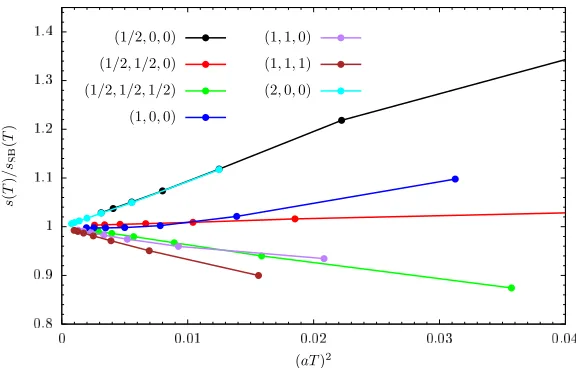
In Figure1we show the continuum limit of the ratio of the entropy density computed at the lowest order in lattice perturbation theory through Eq. (2), and the expected continuum limit, namely the Stefan-Boltzmann (SB) result for QCD withNfquark-flavours:
sSB(T)
T3 = π2 45
32
+21×Nf. (6)
Specifically, we present data for the relevant case ofNf =3, and different choices of shift vectorξ. We considered lattices withL0/a=4, . . . ,16, and a fixed ratioL/L0=32; with this choice finite volume effects can be ignored in the present discussion. The results are plotted against the temperatureT in lattice units (cf. Eq. (2)). It is interesting to note that, in the free case and forNf =3, the fermionic contribution to the entropy density is twice as larger than the gluonic one. In particular, not only the physical component of the entropy is dominated by the quark sector, but also its lattice artifacts. Nonetheless, the cases withξ =(1,0,0) and (1/2,1/2,0) appear to have in general very small lattice artifacts: below 5% for (aT)2<0.02. For these shift vectors, the latter condition translates into having lattices withL0/a≥6, for which discretization errors are about 2% or below. Moreover, we note that the approach to the continuum limit is clearly O(a2). This is expected since, in perturbation theory, the O(a) effects in this quantity are all of O(amq), wheremqis the subtracted bare quark mass. These
effects are hence absent in the chiral limit.
4 Simulation results
The numerical simulations have been performed using a customized version of theopenQCD-1.6
package [22,23]. This allowed us to employ several efficient algorithms to speed up the simula-tions. More precisely, the simulation of the doublet of up and down quarks employed an optimized twisted-mass Hasenbusch preconditioning of the quark determinant [24], while the strange quark was simulated through a RHMC algorithm [25,26] with an optimized frequency splitting of the rational approximation. Even-odd preconditioning was used for both the light and strange quarks. The in-tegration of the molecular dynamics equations was based on a three-level inin-tegration scheme. The gauge force was integrated on the finest level using a 4th-order Omelyan-Mryglod-Folk (OMF4) inte-grator [27], while the fermionic forces were integrated on the two coarser levels. On the finest of these we used a OMF4 integrator, while on the coarsest a 2nd-order OMF integrator [27]. The solution of the Dirac equation along the molecular dynamics evolution was obtained using a standard conjugate gradient with chronological inversion. More details on the exact implementation of these algorithms can be found in the references provided.
In order to access the feasibility of a determination of the EoS in 3-flavour QCD with Wilson fermions and SBC, the first crucial issue to be addressed is the computational effort necessary to obtain a given statistical precision for the basicbarequantitiesTF,G
0k ξ; particularly important is how this
depends on the temperature. We considered three different ensembles of well separated temperatures; a detailed description is given below. For all simulations we choseξ = (1,0,0), L0/a = 6, and
In Figure1we show the continuum limit of the ratio of the entropy density computed at the lowest order in lattice perturbation theory through Eq. (2), and the expected continuum limit, namely the Stefan-Boltzmann (SB) result for QCD withNf quark-flavours:
sSB(T)
T3 = π2 45
32
+21×Nf. (6)
Specifically, we present data for the relevant case ofNf =3, and different choices of shift vectorξ. We considered lattices withL0/a=4, . . . ,16, and a fixed ratioL/L0 =32; with this choice finite volume effects can be ignored in the present discussion. The results are plotted against the temperatureT in lattice units (cf. Eq. (2)). It is interesting to note that, in the free case and forNf =3, the fermionic contribution to the entropy density is twice as larger than the gluonic one. In particular, not only the physical component of the entropy is dominated by the quark sector, but also its lattice artifacts. Nonetheless, the cases withξ=(1,0,0) and (1/2,1/2,0) appear to have in general very small lattice artifacts: below 5% for (aT)2<0.02. For these shift vectors, the latter condition translates into having lattices withL0/a≥6, for which discretization errors are about 2% or below. Moreover, we note that the approach to the continuum limit is clearly O(a2). This is expected since, in perturbation theory, the O(a) effects in this quantity are all of O(amq), wheremqis the subtracted bare quark mass. These
effects are hence absent in the chiral limit.
4 Simulation results
The numerical simulations have been performed using a customized version of theopenQCD-1.6
package [22,23]. This allowed us to employ several efficient algorithms to speed up the simula-tions. More precisely, the simulation of the doublet of up and down quarks employed an optimized twisted-mass Hasenbusch preconditioning of the quark determinant [24], while the strange quark was simulated through a RHMC algorithm [25,26] with an optimized frequency splitting of the rational approximation. Even-odd preconditioning was used for both the light and strange quarks. The in-tegration of the molecular dynamics equations was based on a three-level inin-tegration scheme. The gauge force was integrated on the finest level using a 4th-order Omelyan-Mryglod-Folk (OMF4) inte-grator [27], while the fermionic forces were integrated on the two coarser levels. On the finest of these we used a OMF4 integrator, while on the coarsest a 2nd-order OMF integrator [27]. The solution of the Dirac equation along the molecular dynamics evolution was obtained using a standard conjugate gradient with chronological inversion. More details on the exact implementation of these algorithms can be found in the references provided.
In order to access the feasibility of a determination of the EoS in 3-flavour QCD with Wilson fermions and SBC, the first crucial issue to be addressed is the computational effort necessary to obtain a given statistical precision for the basicbarequantitiesTF,G
0k ξ; particularly important is how this
depends on the temperature. We considered three different ensembles of well separated temperatures; a detailed description is given below. For all simulations we choseξ = (1,0,0), L0/a = 6, and
L/a = 96, therefore havingT L ≈11. We note that the leading finite volume effects in the entropy density are exponentially small in the productML, whereMis the lightest screening mass at the given temperature (see [12] for explicit formulas in presence of SBC). Having this noticed, based on the results of finite volume studies conducted in SU(3) Yang-Mills theory [14,17], and on perturbative estimates of the lightest screening masses in QCD [28], we expect finite volume effects to be well below the precision reached in our exploratory runs (see below). Of course, for a precise determination of the entropy density a systematic study of finite volume effects needs to be carried out. In this respect, we emphasize that considering larger spatial volumes is not a real issue in our set-up. Our
computation of the entropy density is based on the measurement of a simple one-point function of the EMT (cf. Eq. (2)). The increase in computational effort due to a larger spatial volume is hence largely compensated by the statistical gain deriving from averaging the one-point function over a larger number of space-time points. Also, simulating large spatial volumes would help in controlling systematic effects arising from the freezing of topology at small lattice spacings [29,30].
Ensemble β csw κud κs
T1† 3.5500 1.824865382 0.137080000 0.136840284
T2 6.4680 1.409845309 0.135201231 0.135201231
T3 8.0891 1.255925917 0.132802475 0.132802475 †This ensemble employs the Lüscher-Weisz gauge action instead of Wilson’s plaquette.
Table 1.Bare action parameters for the simulated ensembles at temperatures:T1,T2,T3. As usual,β=6/g20, andκ−1=2m
0+8, withm0the bare quark mass of either the up and down quarks (ud) or the strange quark (s). cswdenotes the improvement coefficient of the Sheikholeslami-Wohler term.
We shall now describe in some detail the three ensembles we considered.
1. T1: The lattice bulk-action and action bare parameters of this ensemble match those of ensemble N203 of CLS [31,32]. Specifically, the simulations employNf =2+1 non-perturbatively O(a )-improved Wilson fermions and the Symanzik tree-level O(a2)-improved (Lüscher-Weisz) gauge action (see the given references for more details). The bare action parameters are reported in Table1for the reader’s convenience. These correspond to having a lattice spacinga≈0.064 fm, and quark masses such that mπ ≈ 340 MeV andmK ≈ 440 MeV atT = 0. The resulting
temperature with our choiceL0/a=6 andξ=(1,0,0) isT1≈0.36 GeV.
2. T2: For this ensemble the bare coupling was fixed by requiring the Schödinger functional (SF) coupling at the energy scaleµ0 = T2×3√2/4 to have the value ¯g2SF(µ0) = 2.012 [33,34]. From the results of [35] one infers thatT2 ≈ 4 GeV. The bare quark masses were all set to approximatively their critical value, hence simulating the theory at very small quark masses. This was feasible since at high temperature the massless Dirac operator develops a spectral gap λ∝T.1 The critical mass was estimated by extrapolating to infinite volume the results obtained
in finite volume SF simulations [34].2 The precise set of parameters considered is given in
Table1. In this respect, we must note that using the results for the quark-mass renormalization determined along the lines of constant physics defined through the SF couplings [36], it will be possible in future runs to tune the quark masses to the their physical values over a wide range of temperatures, i.e. up toT ≈70 GeV.3
3. T3: Analogously to the case of the T2 ensemble, also for this ensemble we fixed the bare coupling through the SF coupling, having ¯g2SF(µ)≈1.27 withµ=T3×3√2/4. This corresponds toT3≈45 GeV [33,35]. The quark masses were all set (approximatively) to their critical value, estimated from small volume SF simulations (cf. Table1).
1At lowest order in perturbation theoryλ=πT.
2In principle there is no need to extrapolate the results for the critical mass determined in small volume SF simulations to infinite volume, as the volume dependence is a pure lattice artifacts. By performing an infinite volume extrapolation, however, we aimed at reducing such lattice effects.
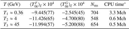
T(GeV) TF
0kξ×104 T0Gkξ×104 Nms CPU time∗
T1 ≈0.36 −9.445(77) −2.545(45) 704 3.3 Mch
T2 ≈4 −11.426(65) −4.700(80) 548 0.6 Mch
T3 ≈45 −11.994(57) −5.200(88) 654 0.5 Mch ∗Simulations performed at Marconi (CINECA) using 4096 cores of Intel Xeon
Phi 7250 Knights Landing (KNL) processors.
Table 2.Results for the bare expectation valuesTF,G
0k ξat the three chosen temperatures:T1,T2,T3. A total of Nmsmeasures was considered, each separated by 10 MDU. The estimated CPU time required for the generation
of the ensembles is also given.
The results for the bare expectation valuesTF,G
0k ξcorresponding to the ensemblesT1,T2,T3are given in Table2. The table provides the total number of measurements gathered. These were collected every 10 MDU along the Monte Carlo histories, detecting no autocorrelations. In the table we also report the CPU time invested in the calculations. As one can see, the figures are modest, while the statistical precision reached on the bare quantities is remarkable: 0.5−1%, depending on the temperature, for the fermionic contributionTF
0kξ, and slightly below 2% for the gluonic contribution
TG
0kξ. The results are particularly encouraging since, as expected forNf = 3 QCD, the fermionic
contribution to the entropy is significantly larger than the gluonic one, but it can be determined more accurately for a given number of independent measurements, especially at high temperature.
A few miscellaneous observations are in order at this point. Firstly, if we had measured the observables more frequently, we would have obtained a significantly better precision at essentially the same computational cost. AtT2 andT3 for example, we observed that the autocorrelations of
TF,G
0k are in fact below 2 MDU: much shorter than we originally expected. As the generation of a
gauge configuration is for all ensembles substantially more expensive than the measurement of the observables (about a factor 9 larger), measuring every 2 MDU instead of 10 MDU would reduce the computational effort necessary to obtain a given statistical precision by an interesting factor. Secondly, for these exploratory runs we did not consider any optimization of our code to run on KNL processors. Another interesting speed-up factor might thus be obtained even with a basic optimization strategy.4
When moving from intermediate to high temperatures we observe that a precise determination of the bare expectation valuesTF,G
0k ξbecomes easier. The main reasons is because the simulations do become easier. This is so because the theory to be simulated approaches the simple free theory, and the spectral gap of the Dirac operator gets larger as the temperature increases; this is a similar situation to step-scaling simulations with the SF [33,34]. In addition, we note that the relative error of the fermionic contributionTF
0kξdecreases for a given number of independent measurements.
Finally, it is also interesting to note that the simulation algorithm appears to sample topology well at the lowest temperatureT1, wherea ≈ 0.064 fm. There we find: Q2ξ = 5.2(3).5 At the higher temperaturesT2 andT3, however, quantitative conclusions cannot be drawn. Certainly, one would expect topology to be very much suppressed at these high temperatures, but concurrently the simulation algorithm must suffer from a severe freezing of the topology at these very small lattice spacings [38,39]. All we can say is that our runs seem to exclusively sample theQ=0 sector.
4By comparing timings obtained on the KNL processors at Marconi with those obtained on our local cluster of Intel Xeon E5-2630 and Intel Xeon E5-2650 processors, we estimated a loss in performances by a factor 2−3.
T(GeV) TF
0kξ×104 T0Gkξ×104 Nms CPU time∗
T1≈0.36 −9.445(77) −2.545(45) 704 3.3 Mch
T2≈4 −11.426(65) −4.700(80) 548 0.6 Mch
T3≈45 −11.994(57) −5.200(88) 654 0.5 Mch ∗Simulations performed at Marconi (CINECA) using 4096 cores of Intel Xeon
Phi 7250 Knights Landing (KNL) processors.
Table 2.Results for the bare expectation valuesTF,G
0k ξat the three chosen temperatures:T1,T2,T3. A total of Nmsmeasures was considered, each separated by 10 MDU. The estimated CPU time required for the generation
of the ensembles is also given.
The results for the bare expectation valuesTF,G
0k ξcorresponding to the ensemblesT1,T2,T3are given in Table2. The table provides the total number of measurements gathered. These were collected every 10 MDU along the Monte Carlo histories, detecting no autocorrelations. In the table we also report the CPU time invested in the calculations. As one can see, the figures are modest, while the statistical precision reached on the bare quantities is remarkable: 0.5−1%, depending on the temperature, for the fermionic contributionTF
0kξ, and slightly below 2% for the gluonic contribution
TG
0kξ. The results are particularly encouraging since, as expected forNf = 3 QCD, the fermionic
contribution to the entropy is significantly larger than the gluonic one, but it can be determined more accurately for a given number of independent measurements, especially at high temperature.
A few miscellaneous observations are in order at this point. Firstly, if we had measured the observables more frequently, we would have obtained a significantly better precision at essentially the same computational cost. AtT2 andT3 for example, we observed that the autocorrelations of
TF,G
0k are in fact below 2 MDU: much shorter than we originally expected. As the generation of a
gauge configuration is for all ensembles substantially more expensive than the measurement of the observables (about a factor 9 larger), measuring every 2 MDU instead of 10 MDU would reduce the computational effort necessary to obtain a given statistical precision by an interesting factor. Secondly, for these exploratory runs we did not consider any optimization of our code to run on KNL processors. Another interesting speed-up factor might thus be obtained even with a basic optimization strategy.4
When moving from intermediate to high temperatures we observe that a precise determination of the bare expectation valuesTF,G
0k ξbecomes easier. The main reasons is because the simulations do become easier. This is so because the theory to be simulated approaches the simple free theory, and the spectral gap of the Dirac operator gets larger as the temperature increases; this is a similar situation to step-scaling simulations with the SF [33,34]. In addition, we note that the relative error of the fermionic contributionTF
0kξdecreases for a given number of independent measurements.
Finally, it is also interesting to note that the simulation algorithm appears to sample topology well at the lowest temperatureT1, wherea ≈ 0.064 fm. There we find: Q2ξ = 5.2(3).5 At the higher temperaturesT2 andT3, however, quantitative conclusions cannot be drawn. Certainly, one would expect topology to be very much suppressed at these high temperatures, but concurrently the simulation algorithm must suffer from a severe freezing of the topology at these very small lattice spacings [38,39]. All we can say is that our runs seem to exclusively sample theQ=0 sector.
4By comparing timings obtained on the KNL processors at Marconi with those obtained on our local cluster of Intel Xeon E5-2630 and Intel Xeon E5-2650 processors, we estimated a loss in performances by a factor 2−3.
5We monitored topology by means of the topological chargeQdefined through the Yang-Mills gradient flow [37]. In particular, we measure the topological charge at flow-time√8t=0.4×T−1, anddefinethe “Q=0 sector” as the set of gauge configurations for which|Q|<0.5.
5 Conclusions
The results we presented show that within the framework of SBC, a precision of 0.5−1% on the bare quantities entering the determination of the entropy density is reachable with modest computational effort and over a wide range of temperatures, easily covering two orders of magnitude in the tempera-ture. This is very encouraging in view of a precise determination of the EoS ofNf =2+1 QCD using non-perturbatively O(a)-improved Wilson fermions. In particular, differently from the situation that occurs with more standard methods, the higher the temperature is, the easier the simulations become, and thus the easier is to obtain precise results. The fundamental reason for this favorable situation is that the problem of computing the bare expectation values and their renormalization are completely disentangled in our framework, and can therefore be tackled separately. The important question at this point is hence whether the necessary renormalization of the EMT can be obtained with a competitive level of precision. This issue is under current investigation and the details of our renormalization strategy are in preparation [40].
Regarding the renormalization of the EMT we must note that several interesting ideas, based on the Yang-Mills gradient flow [37], have been proposed [41–43] (see [44] for a review). Following some of these strategies promising results for the EoS have already been obtained, both in SU(3) Yang-Mills theory and QCD [45,46]. From a different perspective, other promising ideas for determining the EoS have been devised and tested [47,48].
Finally, another important issue we shall address in order to obtain an accurate determination of the EoS using Wilson fermions is a systematic study of the O(a)-improvement of the EMT. In this respect, it is interesting to note that chiral symmetry “restoration” at high temperature may have interesting consequences on the lattice artifacts of the theory. Following standard arguments [49], one expects indeed some degree of “automatic” O(a)-improvement at high temperature [40].
6 Acknowledgements
The authors thank Bastian Brandt for discussion on the development of the code. M.D.B. would like to express his gratitude to the Theoretical Physics Department at CERN for the hospitality extended to him, and also thanks Stefan Sint for interesting discussions. The code used for the generation of the ensembles is based on theopenQCD-1.6 package [23]. Numerical calculations have been made possible through a CINECA-INFN agreement, providing access to resources on GALILEO and MARCONI at CINECA. The authors are also grateful to the computer centers at the University of Milano-Bicocca and CERN for their valuable support and resources.
References
[1] A. Dainese et al., CERN Yellow Report pp. 635–692 (2017)
[2] K. Kajantie, M. Laine, K. Rummukainen, Y. Schröder, Phys. Rev.D67, 105008 (2003) [3] J.P. Blaizot, E. Iancu, A. Rebhan, Phys. Rev.D68, 025011 (2003)
[4] J.O. Andersen, M. Strickland, Annals Phys.317, 281 (2005) [5] S. Borsanyi et al., Phys. Lett.B730, 99 (2014)
[6] G.S. Bali, F. Bruckmann, G. Endrödi, S.D. Katz, A. Schäfer, JHEP08, 177 (2014) [7] A. Bazavov et al. (HotQCD), Phys. Rev.D90, 094503 (2014)
[8] G. Boyd et al., Nucl. Phys.B469, 419 (1996)
[9] A. Bazavov, P. Petreczky, J.H. Weber (2017),1710.05024
[11] L. Giusti, H.B. Meyer, JHEP11, 087 (2011) [12] L. Giusti, H.B. Meyer, JHEP01, 140 (2013)
[13] D. Robaina, H.B. Meyer, PoSLATTICE2013, 323 (2014) [14] L. Giusti, M. Pepe, Phys. Rev. Lett.113, 031601 (2014) [15] T. Umeda, Phys. Rev.D90, 054511 (2014)
[16] L. Giusti, M. Pepe, Phys. Rev.D91, 114504 (2015) [17] L. Giusti, M. Pepe, Phys. Lett.B769, 385 (2017)
[18] L.D. Landau, E.M. Lifschits,Fluid Mechanics, Vol. 6 ofCourse of Theoretical Physics (Perga-mon Press, Oxford, 1975), ISBN 9780080181769
[19] S. Caracciolo, G. Curci, P. Menotti, A. Pelissetto, Annals Phys.197, 119 (1990) [20] S. Caracciolo, P. Menotti, A. Pelissetto, Phys. Lett.B260, 401 (1991)
[21] S. Caracciolo, P. Menotti, A. Pelissetto, Nucl. Phys.B375, 195 (1992) [22] M. Lüscher, S. Schaefer, Comput. Phys. Commun.184, 519 (2013) [23] openQCD package,http://luscher.web.cern.ch/luscher/openQCD [24] M. Hasenbusch, Phys. Lett.B519, 177 (2001)
[25] A.D. Kennedy, I. Horváth, S. Sint, Nucl. Phys. Proc. Suppl.73, 834 (1999) [26] M.A. Clark, A.D. Kennedy, Nucl. Phys. Proc. Suppl.129, 850 (2004)
[27] I.P. Omelyan, I.M. Mryglod, R. Folk, Comp. Phys. Commun.151, 272 (2003) [28] M. Laine, M. Vepsalainen, JHEP09, 023 (2009)
[29] R. Brower, S. Chandrasekharan, J.W. Negele, U.J. Wiese, Phys. Lett.B560, 64 (2003)
[30] M. Lüscher,Stochastic locality and master-field simulations of very large lattices, in Proceed-ings,35th International Symposium on Lattice Field Theory (Lattice2017): Granada, Spain, June 18-24, 2017, to appear in EPJ Web Conf.,1707.09758
[31] M. Bruno et al., JHEP02, 043 (2015)
[32] M. Bruno, T. Korzec, S. Schaefer, Phys. Rev.D95, 074504 (2017) [33] M. Dalla Brida et al. (ALPHA), Phys. Rev. Lett.117, 182001 (2016) [34] M. Dalla Brida et al. (ALPHA), Phys. Rev.D95, 014507 (2017) [35] M. Bruno et al. (ALPHA), Phys. Rev. Lett.119, 102001 (2017) [36] I. Campos et al., PoSLATTICE2016, 201 (2016)
[37] M. Lüscher, JHEP08, 071 (2010), [Erratum: JHEP 03, 092 (2014)] [38] L. Del Debbio, H. Panagopoulos, E. Vicari, JHEP08, 044 (2002)
[39] S. Schaefer, R. Sommer, F. Virotta (ALPHA), Nucl. Phys.B845, 93 (2011) [40] M. Dalla Brida, L. Giusti, M. Pepe, in preparation
[41] H. Suzuki, PTEP2013, 083B03 (2013), [Erratum: PTEP 2015, 079201 (2015)]
[42] H. Makino, H. Suzuki, PTEP2014, 063B02 (2014), [Erratum: PTEP 2015, 079202 (2015)] [43] L. Del Debbio, A. Patella, A. Rago, JHEP11, 212 (2013)
[44] H. Suzuki, PoSLATTICE2016, 002 (2017) [45] Y. Taniguchi et al., Phys. Rev.D96, 014509 (2017)
[46] M. Kitazawa, T. Iritani, M. Asakawa, T. Hatsuda, H. Suzuki, Phys. Rev.D94, 114512 (2016) [47] M. Caselle, G. Costagliola, A. Nada, M. Panero, A. Toniato, Phys. Rev.D94, 034503 (2016) [48] A. Nada, M. Caselle, M. Panero,The equation of state with non-equilibrium methods, in
Pro-ceedings,35th International Symposium on Lattice Field Theory (Lattice2017): Granada, Spain, June 18-24, 2017, to appear in EPJ Web Conf.,1710.04435