LAPLACE TRANSFORM AND ITS APPLICATIONS

(1)

179 | P a g e

LAPLACE TRANSFORM AND ITS APPLICATIONS

Manchala Sabitha

Dept of Mathematics. DIET, Hyderabad (India)

ABSTRACT

An introduction to Laplace Transform is the topic of this paper. It deals with what Laplace Transform is, and

what is it actually used for. The definition of Laplace Transform and most of its important properties have been

mentioned with detailed proofs. This paper also includes a brief overview of Inverse Laplace Transform. A

number a methods used to find the time domain function from its frequency domain equivalent have been

explained with detailed explanations. It also includes the formulation of Laplace Transform of certain special

function like the Heaviside’s Unit Step Function and the Dirac Delta Function. A few practical life applications

of Laplace Transform have also been stated.

Keywords: Laplace Transform, Heaviside’s, properties, Dirac Delta.

I. INTRODUCTION

This paper deals with a brief overview of what Laplace Transform is and its application in the industry. The Laplace Transform is a specific type of integral transform. Considering a function f (t), its corresponding Laplace Transform will be denoted as L[f(t)], where L is the operator operated on the time domain function f(t). The Laplace Transform of a function results in a new function of complex frequency s. Like the Fourier Transform, the Laplace Transform is also used in solving differential and integral equations. It is also predominantly used in the analysis of transient events in the electrical circuits where frequency domain analysis is used.Important analytical method for solving linear ordinary differential

II. DEFINITION OF LAPLACE TRANSFORM

Consider a function of time f(t). If this function satisfies certain conditions and if the integral, ∅(s) = 𝑒₀∞ −𝑠𝑡𝑓 𝑡 𝑑𝑡 Exists, then ∅(s) represents the Laplace Transform of f(t), i.eL[f(t)]= 𝑒₀∞ −𝑠𝑡𝑓(𝑡)𝑑𝑡 …(1)

III. PROPERTIES AND THEOREMS OF LAPLACE TRANSFORM

3.1 Linearity Property: If𝑘₁ and 𝑘₂ are constants, then, 𝐿[𝑘₁𝑓₁ 𝑡 + 𝑘₂𝑓₂ 𝑡 = 𝑘₁𝐿 𝑓₁ 𝑡 +

𝑘2𝐿[𝑓2(𝑡)]………(2)

3.2 Change of Scale Property:

A linear multiplication or division of a constant with the

variable is known as scaling. Thus, ife L[f(t)]=∅(s) then by change of scale property,𝐿 𝑓 𝑎𝑡 =

1 𝑎∅

𝑠

𝑎 … … … (3)

3.3 First Shifting Theorem

(2)

180 | P a g e

3.4 Second Shifting Theorem

The Second Shifting Theorem of Laplace Transform states that ifL[f(t)]=∅(s), then the Laplace Transform of thefollowing function,𝑔 𝑡 = 𝑓 𝑡 − 𝑎 𝑤𝑕𝑒𝑛 𝑡 > 𝑎 𝑎𝑛𝑑 𝑔 𝑡 = 0 𝑤𝑕𝑒𝑛 𝑡 < 𝑎.Is expressed as L[g(t)]=𝑒−𝑎𝑠∅(𝑠)………….(5)

3.5 Multiplication of powers of the variable

The variable that has been used so far is‘t’. Thus, if wemultiply powers of t with the original function f (t),

theLaplace transform can be expressed as𝐿 𝑡𝑛𝑓 𝑡 = −1 𝑛 𝑑

𝑛

𝑑𝑠𝑛∅ 𝑠 … … . 6 3.6 Division of variable

If L[f(t)]=∅(s), then the Laplace Transform when thefunction is divided by the variable can be expressed as𝐿 𝑓 𝑡

𝑡 = ∅ 𝑠 … … . (7)

∞

𝑠

IV. LAPLACE TRANSFORM OF DERIVATIVES

Let f (t) be the time domain function. The LaplaceTransform of its derivative can be expressed as𝐿 𝑓/ 𝑡 =

𝑠𝐿 𝑓 𝑡 − 𝑓 0 … … … . . (8)

V. LAPLACE TRANSFORM OF INTEGRALS

When the time domain function is integrated, its LaplaceTransform can be expressed as,𝐿[ 𝑓 𝑢 𝑑𝑢] =₀𝑡

1𝑠∅𝑠…….(9)

VI. INVERSE LAPLACE TRANSFORM

6.1 Definition

If L[f(t)] = ∅(s) = 𝑒₀∞ −𝑠𝑡𝑓 𝑡 𝑑𝑡, then f (t) is called theInverse Laplace Transform of∅(𝑠). It can be denoted as,𝐿−1 ∅ 𝑠 = 𝑓 𝑡 … … … . (10)

Thus, the frequency domain function ∅(s) can beconverted to its corresponding time domain equivalent f Converted to its corresponding time domain equivalent f(t) using the Laplace Inverse operator (𝐿−1).

VI. DIFFERENT METHODS OF OBTAINING INVERSE LAPLACE TRANSFORM

There are numerous ways to obtain the Inverse Laplace Transform of a given frequency domain function. The choice of the method employed in solving a problem on Inverse Laplace Transform depends on the nature and structure of the problem itself. Often it would be notedthat a single problem can be solved by multiple methods .A few methods have been explained below.

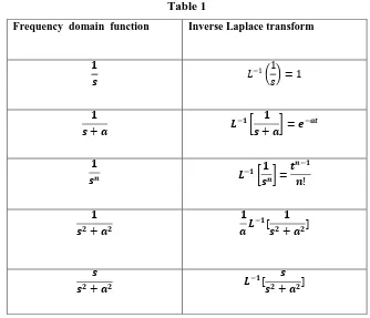
7.1 Using Standard Results

(3)

181 | P a g e

Table 1

7.2 Using First Shifting Theorem

First Shifting Theorem can be expressed as, 𝐿[𝑒−𝑎𝑡f(t)]=∅ 𝑠 + 𝑎 this means that if f(t)=𝐿−1 ∅ 𝑆 then𝐿−1 ∅ 𝑆 + 𝑎 = 𝑒−𝑎𝑡𝑓 𝑡 = 𝑒−𝑎𝑡𝐿−1 ∅ 𝑠 ………..(11)

7.3 Use of Partial Fractions

Whenever possible, it is always easier to solve a problem on Inverse Laplace Transform by expressing the given function ∅(s) into a sum of linear or quadratic partial fraction as,

∅(s) = 𝐴

(𝑠+𝑎)𝑟 + 𝐵𝑠+𝑐

(𝑠2+_𝑎2₎𝑟 and then use standard results given in table 1 to find corresponding Inverse Laplace

Transform.

7.4 Using Change of Scale Property

From equation 3, the change of scale property can be expressed as,L[f(at)]=1_𝑎∅(_𝑎𝑠)

Thus if f(t) =𝐿−1 [ ∅(s) ], taking Inverse Laplace Transform,𝐿−1[_𝑎1∅(_𝑎𝑠)]=f(at)…….(12)

7.5 Convolution Theorem

7.5.1 Definition

If 𝑓1 𝑡 𝑎𝑛𝑑 𝑓2(𝑡) and are two functions, then the following integral 𝑓₀𝑡 1 𝑢 𝑓2 𝑡 − 𝑢 𝑑𝑢

Is called the convolution of 𝑓1 𝑡 𝑎𝑛𝑑 𝑓2 𝑡 and is denoted

as𝑓₁ 𝑡 * 𝑓₂ 𝑡

∴𝑓1(𝑡)∗𝑓2(𝑡)) = 𝑓1 𝑢 𝑓2 𝑡 − 𝑢 𝑑𝑢 𝑡

0 …….(13) 7.5.2 Theorem

Let L[𝑓1(𝑡)] = ∅1(𝑠) 𝑎𝑛𝑑 𝐿[𝑓2(𝑡)] = ∅2(𝑠) 𝑡𝑕𝑒𝑛 𝐿−1[∅1 𝑠 ∅2 𝑠 = 𝑓₀𝑡 1 𝑢 𝑓2 𝑡 − 𝑢 𝑑𝑢…(14)

Where 𝑓1 𝑡 = 𝐿−1 ∅1 𝑠 𝑎𝑛𝑑𝑓2 𝑡 = 𝐿−1[∅2 𝑠 ]

Frequency domain function Inverse Laplace transform

𝟏

𝒔 𝐿−1

1 𝑠 = 1

𝟏

𝒔 + 𝒂 𝑳−𝟏

𝟏

𝒔 + 𝒂 = 𝒆−𝒂𝒕

𝟏

𝒔𝒏 𝑳−𝟏

𝟏 𝒔𝒏 =

𝒕𝒏−𝟏

𝒏!

𝟏 𝒔𝟐_{+ 𝒂}𝟐

𝟏 𝒂𝑳−𝟏[

𝟏 𝒔𝟐_{+ 𝒂}𝟐]

𝒔

𝒔𝟐_{+ 𝒂}𝟐 𝑳−𝟏[

(4)

182 | P a g e

7.6 Using Differentiation of ∅(s)

If L[f(s)] = ∅(s), then using n=1 in equation 6,L[t f(t)]=-∅1(𝑠)

∴𝑡 𝑓 𝑡 = −𝐿−1_[∅1_{𝑠 ]}

∴𝑡 𝐿−1_{[∅ 𝑠 = −𝐿}−1_[∅1_{𝑠 ]}

∴𝐿−1_[∅_{(s)] = -}1 𝑡𝐿

−1_[∅1_{𝑠 ]}_{…….. (15)}

This method is particularly used to find the Inverse Laplace Transform of functions having

𝑡𝑎𝑛−1_{𝑥, 𝑐𝑜𝑡}−1_{𝑥 𝑎𝑛𝑑 𝑙𝑜𝑔𝑥 𝑡𝑒𝑟𝑚𝑠.} 7.7 Using Integration of f (t)

Equation (9) gives us the result of the Laplace Transform when the function f (t) is integrated as

shown,L[ 𝑓₀𝑡 𝑢 𝑑𝑢] =1

𝑠∅(𝑠)

∴ 𝑓 𝑢 𝑑𝑢 = 𝐿−1 1 𝑆∅(𝑠)] 𝑡

0 But by definition, f(u) =𝐿−1 [∅(s)]

∴𝐿−1 1

𝑆∅ 𝑠 = 𝐿

−1_{∅ 𝑠 𝑑𝑠 … . . (16)} 𝑡

0

VIII. LAPLACE TRANSFORM OF PERIODIC FUNCTIONS

Considering f (t) to be a periodic function with period a, it’s Laplace Transform can be expressed as,𝐿 𝑓 𝑡 =

1

1−𝑒−𝑎𝑠 𝑒−𝑠𝑡 𝑎

0 𝑓 𝑡 𝑑𝑡….. (17).

IX. HEAVISIDE’S UNIT STEP FUNCTION

Heaviside’s Unit Step Function can have only two possible values either 0 or 1. It can be defined as, 𝐻 𝑡 = 0, 𝑡 < 0

1, 𝑡 ≥ 0The function takes a jump of unit magnitude at x=0.

Taking the Laplace transform of the above function

L[H(t)]= 𝑒₀∞ −𝑠𝑡H(t)dt

∴𝐿 𝐻 𝑡 = 𝑒∞ −𝑠𝑡

0 dt

= L[1]

∴L[H(t)]=1

𝑠 …....(18)

X. IMPULSE FUNCTION (OR DIRAC DELTA FUNCTION)

The impulse function is obtained by taking the limit of the rectangular pulse as its width, tw, goes to zero but holding the area under the pulse constant at one.

Solution of ODEs by Laplace Transforms Procedure:

 Take the L of both sides of the ODE.

 Rearrange the resulting algebraic equation in the s domain to solve for the L of the output variable, e.g., Y(s).

 Perform a partial fraction expansion.

(5)

183 | P a g e

XI. APPLICATIONS

Laplace Transforms are put to incredible amount of use insolving differential equations and in circuit analysis whichinvolves the components like resistors, inductors and capacitors. Most often, during circuit analysis, the timedomain equations are first written and then Laplace Transform of the time domain equation is taken to convertit to its frequency domain equivalent. However, it is alsopossible to convert the circuit impedance into itsfrequency domain equivalent and then proceed, both ofwhich produce the same result.

XII. CONCLUSION

This paper thus, consisted of a brief overview of what Laplace Transform is, and what is it used for. The primary use of Laplace Transform of converting a time domain function into its frequency domain equivalent was also discussed. Major properties of Laplace Transform and a few special functions like the Heaviside’s Unit Step Function and Dirac Delta Functions were also discussed in detail. It also included a detailed explanation of Inverse Laplace Transform and the various methods that can be employed in finding the Inverse Laplace Transform. It goes without saying that Laplace Transform is put to tremendous use in many branches of Applied Sciences.

REFERENCES

[1] www.tutorial.math.lamar.edu [2] www.sosmath.com

[3] Prof. Algonda Desai, Msc. Mathematics