GENOMIC SELECTION
DAIRRy-BLUP: A High-Performance Computing
Approach to Genomic Prediction
Arne De Coninck,*,1Jan Fostier,†Steven Maenhout,‡and Bernard De Baets* *Research Unit Knowledge-based Systems KERMIT, Department of Mathematical Modelling, Statistics and Bioinformatics, Ghent University, B-9000 Ghent, Belgium,†IBCN, Internet Based Communication Networks and Services Research Unit Department of Information Technology, Ghent University–iMinds, B-9000 Ghent, Belgium, and‡Progeno, B-9052 Zwijnaarde, Belgium
ABSTRACTIn genomic prediction, common analysis methods rely on a linear mixed-model framework to estimate SNP marker effects and breeding values of animals or plants. Ridge regression–best linear unbiased prediction (RR-BLUP) is based on the assumptions that SNP marker effects are normally distributed, are uncorrelated, and have equal variances. We propose DAIRRy-BLUP, a parallel, Distributed-memory RR-BLUP implementation, based on single-trait observations (y), that uses the Average Information algorithm for restricted maximum-likelihood estimation of the variance components. The goal of DAIRRy-BLUP is to enable the analysis of large-scale data sets to provide more accurate estimates of marker effects and breeding values. A distributed-memory framework is required since the dimensionality of the problem, determined by the number of SNP markers, can become too large to be analyzed by a single computing node. Initial results show that DAIRRy-BLUP enables the analysis of very large-scale data sets (up to 1,000,000 individuals and 360,000 SNPs) and indicate that increasing the number of phenotypic and genotypic records has a more significant effect on the prediction accuracy than increasing the density of SNP arrays.
I
N thefield of genomic prediction, genotypes of animals or plants are used to predict either phenotypic properties of new crosses or estimated breeding values (EBVs) for detecting superior parents. Since quantitative traits of importance to breeders are mostly regulated by a large number of loci (QTL), high-density SNP markers are used to genotype individuals [e.g.,.2000 QTL are already found to contribute to the composition and production of milk in cattle (http://www. animalgenome.org/cgi-bin/QTLdb/BT/index)]. The most frequently used SNP arrays for cattle consist of 50,000 SNP markers, but even genotypes with 700,000 SNPs are al-ready available (Cole et al.2012).Some widely used analysis methods rely on a linear mixed-model backbone (Meuwissenet al.2001) in which the SNP marker effects are modeled as random effects, drawn from
a normal distribution. The predictions of the marker effects are known as best linear unbiased predictions (BLUPs), which are linear functions of the response variates. It has been shown that when no major genes contribute to the trait, Bayesian predictions and BLUP result in approximately the same prediction accuracy for the EBVs (Hayeset al.2009; Legarra
et al.2011; Daetwyleret al.2013).
At Present the number of individuals included in the genomic prediction setting is still an order of magnitude smaller than the number of genetic markers on widely used SNP arrays, favoring algorithms that directly estimate EBVs, which is in this case computationally more efficient thanfirst estimating the marker effects (VanRaden 2008; Misztalet al.
2009; Piepho 2009; Shen et al.2013). Nonetheless, it has been shown theoretically (Hayeset al.2009) that to increase the prediction accuracy of the EBVs for traits with a low heritability, the number of genotyped records should in-crease dramatically. Most widely used implementations like synbreed (Wimmeret al.2012) and BLUPF90 (Misztalet al.
2002) are limited by the computational resources that can be provided by a single workstation. We present DAIRRy-BLUP, a parallel framework that takes advantage of a distributed-memory compute cluster to enable the analysis of
Copyright © 2014 by the Genetics Society of America doi: 10.1534/genetics.114.163683
Manuscript received March 3, 2014; accepted for publication April 10, 2014; published Early Online April 15, 2014.
Supporting information is available online athttp://www.genetics.org/lookup/suppl/ doi:10.1534/genetics.114.163683/-/DC1.
large-scale data sets. DAIRRy-BLUP is an acronym for a Distributed-memory implementation of the Average Informa-tion algorithm for restricted maximum-likelihood estimaInforma-tion of the variance components in a Ridge Regression-BLUP setting based on single-trait observationsy. Additionally, results on simulated data illustrate that the use of such large-scale data sets is warranted as it significantly improves the prediction accuracy of EBVs and marker effects.
DAIRRy-BLUP is optimized for processing large-scale dense data sets with SNP marker data for a large number of individuals (.100,000). Variance components are estimated based on the entire data set, using the average information restricted maximum-likelihood (AI-REML) algorithm. There-fore, it distinguishes itself from other implementations of the AI-REML algorithm that are optimized for sparse settings and are not able to make use of the aggregated compute power of a supercomputing cluster (Misztalet al.2002; Masudaet al.
2013).
All matrix equations in the algorithms used by DAIRRy-BLUP are solved using a direct Cholesky decomposition. Although efficient iterative techniques exist that can reduce memory requirements and calculation time for solving a matrix equation (Legarra and Misztal 2008), the choice for a direct solver is motivated by the use of the AI-REML algorithm for variance component estimation on the entire data set.
Materials and Methods
Simulated data
The simulated data used for benchmarking DAIRRy-BLUP were generated using AlphaDrop (Hickey and Gorjanc 2012), which was put forward by the Genetics Society of America to provide common data sets for researchers to benchmark their methods (De Koning and McIntyre 2012). Since no data sets with.10,000 phenotypic and genotypic records are yet publicly available, this software was used to create data sets with 10,000, 100,000, and 1,000,000 individ-uals of a livestock population genotyped for a varying number of SNP sites (9000, 60,000, and 360,000). AlphaDrop first launches MaCS (Chenet al.2009) to create 4000 haplotypes for each of the 30 chromosomes, using an effective popula-tion size of 1000 for thefinal historical generation, which is then used as the base generation for the next 10 generations under study. The base individuals of a simulated pedigree had their gametes randomly sampled from the 4000 haplo-types per chromosome of the sequence simulation. The ped-igree comprised 10 generations with 10 dams per sire and two offspring per dam, with the number of sires depending on the total number of records that was aimed for (50, 500, or 5000). Genotypes for individuals from subsequent generations were generated through Mendelian inheritance with a recombina-tion probability of 1%/cM. The phenotypes of the individuals were affected by 9000 QTL, randomly selected from the 1,670,000 available segregating sites. The effects of these
QTL were sampled from a normal distribution with mean 0 and standard deviation 1. Final phenotypes based on the QTL effects were generated with a user-defined heritability of 0.25.
When constructing the large-scale data sets, it became clear that AlphaDrop, which is a sequential program and does not make use of any parallel programming paradigm, was not designed for generating SNP data for such large numbers of individuals. The largest data set that could be created consisted of 1,000,000 individuals, each genotyped for 60,000 SNPs. This required118 GB of working mem-ory and thefinal data set was stored in textfiles with a total size of350 GB. The simulation took.13 days on an Intel Xeon E5-2420 1.90 GHz with 64 GB RAM and another 65 GB as swap memory. The data sets can be recreated by using the correct seeds for the random number generators in the MaCS and AlphaDrop software. These seeds and the inputfiles used for creating the data sets with AlphaDrop are enclosed in supporting informationFile S1.
Statistical method: linear mixed model
The underlying framework for the analysis of genotypic data sets is the linear mixed model,
y¼XbþZuþe;
whereyis a vector ofnobservations,bis a vector oftfixed effects,uis a vector ofsrandom effects, andeis the residual error. X and Z are the incidence matrices that couple the effects to the observations. Assuming that the random effects and the residual error are normally distributed,u N ð0;GÞande N ð0;RÞ;the observations are also normally distributed:y N ðXb;VÞ;withV¼RþZGZT:
The BLUPs of the random effects are linear estimates that minimize the mean squared error and exhibit no bias. Henderson (1963) translated this estimation procedure into the so-called mixed-model equations (MMEs), which can be written in matrix form as
"
XTR21X XTR21Z
ZTR21X ZTR21ZþG21 #"^
b ^ u
# ¼
"
XTR21y
ZTR21y #
:
A common simplification, which leads to the ridge regression (RR) formulation (Piepho 2009), is to assume that all SNP marker effects are uncorrelated and have homosce-dastic variance s2u:Similarly, residual errors are assumed to
be uncorrelated and to have homoscedastic variances2
e.
Al-though these assumptions might not be in accordance with reality, it has been shown that this simplified model can reach prediction accuracies that are close to those of more complex models (VanRaden et al. 2009; Shen et al. 2013). The co-variance matrices are thus set toR¼s2eIn (withIn the
iden-tity matrix of dimensionn) andG¼s2uIs;which leads to the
following MME: 2 6 4
XTX XTZ
ZTX ZTZþs2e
s2 u Is 3 7 5 ^ b ^ u ¼
XTy
ZTy
:
The solution to this matrix equation is known as the RR-BLUP, becauses2
e=s2u can be seen as a ridge regression
pe-nalization parameter, which controls the pepe-nalization by the sum of squares of the marker effects. In this case, however, the penalization parameter is not estimated by cross-validation, but since it is a ratio of two variance components, the latter will be estimated by a REML procedure.
In this specific study on simulated data sets, no fixed effects other than the overall mean are modeled;i.e.,t= 1 and X¼1n (vector ofnones). The random effects are the
SNP marker effects and every observation corresponds to the phenotypic score of an individual.
AI-REML
When the covariance structures of the random effects and of the residual errors depend on the respective variance component vectorsgandu,
u e eN
0;s2
GðgÞ 0 0 RðfÞ
;
the REML log-likelihood can be written as
lREMLðs2;g;fÞ
¼ 21 2
ðn2tÞlog s2þlog G þlog R þlog C þy
TPy
s2
(Gilmouret al.1995), whereCis the coefficient matrix from the MME as defined in the previous section and
P¼V212V21XXTV21X21XTV21:
With the aforementioned assumptions and settings2¼s2
e;
R¼In;andG¼gIs;withg¼s2
u=s2e;this simplifies to a
log-likelihood with only two parameters, namelys2
e andg;
lREMLðs2e;gÞ ¼ 2
1 2
ðn2tÞlogs2eþbloggþlog C þy
TPy
s2
e
;
whereCandPdepend only ong. In this form, we canfind an analytical solution for the maximization of the log-likelihood with respect tos2
e;providedgis known:
s2e ¼y
TPy
n2t:
The maximization of the REML log-likelihood function with respect togcan mostly not be solved analytically, due to the complexfirst derivative with respect tog, also known as the score function,
@lREML
@g ¼ 2 1 2
b g2
trðCZZÞ g2 2
^ uTu^
s2eg2
; (1)
with CZZ, the lower right block of the inverse of C, also depending on g. Newton’s method for maximizing likeli-hood functions can be used to find a solution for this opti-mization problem. The iterative scheme looks like
kiþ1¼ki2Hi21=lREMLðkiÞ; (2)
with kithe vector of unknowns [hereki¼ ðs2e;gÞi] at
iter-ation i,Hithe Hessian matrix oflREMLevaluated atki;and
=lREMLðkiÞ the gradient vector of the REML log-likelihood
with respect to k, evaluated at ki: However, the Hessian matrix can be very hard to construct due to the large size of the matrices that need to be multiplied or inverted.
Originally, Patterson and Thompson (1971) used the Fisher information matrix, which is the expected value of the Hessian matrix, for updating the variance components, but the computation of the elements of this Fisher informa-tion matrix involves calculating traces of large matrices, which are tedious to construct. Taking an average of the expected and observed Hessian matrix, these traces disap-pear in the expression of the update matrix. The resulting update matrix is called the AI matrix and it can be shown (Gilmour et al.1995) that this AI matrix can easily be cal-culated as
HAI¼ 1 2s2
e
QTPQ;
with Q¼ y s2 e Z^u g : (3)
A more detailed derivation of the AI matrix can be found in theAppendix.
Not only is the AI-REML procedure computationally practical for use in a distributed-memory framework, but also it has shown that fewer iterations are needed to obtain convergence compared to a derivative-free (DF) algorithm or an expectation-maximization (EM) algorithm (Gilmour
Distributed-memory computing techniques
For large-scale data sets, the application of the RR-BLUP methodology on a single workstation is computationally impractical because of the high memory requirements to store the large and dense coefficient matrixC. To deal with data sets beyond the memory capacity of a single machine, a parallel, distributed-memory implementation was devel-oped. DAIRRy-BLUP can take advantage of the aggregated computing power and memory capacity of a large number of networked machines by distributing both data and compu-tations over different processes, which can be executed in parallel on the central processing unit (CPU) cores of the networked nodes. This allows DAIRRy-BLUP to be executed even on clusters with a low amount of memory per node, because every large matrix in the algorithm is distributed among all parallel processes;i.e., every process holds parts of the matrix and can pass these parts to another process if necessary through message passing (Snir et al. 1995). By default the matrix is split up in blocks of 64364 elements; however, this can be changed in functions of matrix size and computer architecture. More information about how matri-ces are distributed in DAIRRy-BLUP can be found in the
Appendix.
The coefficient matrixChas dimensions of (s+t)3(s+
t), the sum of random andfixed effects; however, to con-struct it, we need to multiply matrices with dimensionss, the number of random effects, byn, the number of individuals, andt, the number offixed effects, byn. In genomic data sets,
s, the number of SNP markers, is usually a lot larger thant
and nowadays nis mostly still smaller thans. However, as discussed in later sections, the number of observations (n) should increase to provide accurate estimates of the marker effects and the resulting breeding values. It is expected that indeed the number of genotyped individuals will increase in the future, since the cost of genotyping is constantly decreas-ing and more data of genotyped animals will be gathered in future years. Therefore, the algorithm is implemented in such a way that the number of observationsn does not have an impact on memory usage. To obtain this, theyvector and the
ZandXmatrices are read from the inputfiles per strip, as was also suggested by Piephoet al.(2012). These strips consist of a certain number of rows, defined by the block size and the number of processes involved. The lower-right block of the coefficient matrixCZZis then calculated as
CZZ¼
Xq
i¼1
ZT
iZiþgIZ; (4)
with qthe number of strips needed to read in the entire Z matrix,Zithe strips of theZmatrix, andIZthe identity matrix
with the same dimensions asCZZ:
All mathematical operations that have to be performed on the distributed matrices rely on the standard distrib-uted linear algebra libraries PBLAS (Choi et al. 1996a) and ScaLAPACK (Blackfordet al.1997). The MMEs are solved through a Cholesky decomposition of the symmetric
coef-ficient matrixC. The AI-REML algorithm iterates until con-vergence of gand since predictions of the marker effects, depending ong, appear in the score function of the AI-REML algorithm, a Cholesky decomposition of the updated coeffi -cient matrix is required each iteration. ScaLAPACK overwrites the original coefficient matrix by its Cholesky decomposition, implyingCto be set up from scratch at the beginning of every iteration. Nonetheless, when sufficient working memory is available and the construction ofCbecomes a time-consuming factor, an option can be enabled in DAIRRy-BLUP to store a copy of the coefficient matrix, which can then rapidly be updated with new values ofgand thus renders a complete setup ofCunnecessary.
Inputfiles
As already mentioned, the data files can require.100 GB of disk space when stored as a textfile. Due to the distrib-uted read-in of the datafiles, DAIRRy-BLUP can only cope with binaryfiles, which may require even more space when the data are stored as 64-bit integers or doubles. To over-come this massive hard disk consumption, DAIRRy-BLUP can read in data in the hierarchical data format (HDF5) (HDF Group 2000–2010). The HDF5file format stores data sets in a file system-like format, providing every data set with a /path/to/resource. Metadata can be added to the data sets in the form of named attributes attached to the path or the data set. It is recommended to use the HDF5file type for analyzing data with DAIRRy-BLUP due to two major advantages.
First, HDF5 offers the possibility to compress data into blocks with the result that up to 10 times less space is consumed by thefinal HDF5file than by storing the data in textfiles. Second, if the size of the compressed blocks is equal to the size of the blocks in which the data are distributed across the memory of all dedicated processes, there is also a significant gain in read-in time of the data. Indeed, every process needs only to decompress several blocks before reading in and does not have to go through the whole data set as is the case when using conventional binaryfiles.
Table 1 Computational demands of DAIRRy-BLUP for different numbers of SNP markers included in the analysis for a population of 100,000 individuals
SNPs Parallel processes Wall time (hr:min:sec) No. iterations RAM per process (MB) Total RAM (GB)
9,000 16 00:10:56 3 93 1.5
60,000 32 02:54:48 2 608 19.5
High-performance computing infrastructure
All results were obtained using the Gengar cluster on Stevin, the high-performance computing (HPC) infrastructure of Ghent University. This cluster consists of 194 computing nodes (IBM HS 21 XM blades) interconnected with a 4X DDR Infiniband network (20 Gbit/sec). Each node contains a dual-socket quad-core Intel Xeon L5420 2.5-GHz CPU (eight quad-cores) with 16 GB RAM. To achieve a high performance a one-to-one mapping of processes to CPU cores was applied and the number of dedicated CPU cores was chosen in such a way that there was a fair balance between wall time and occupation of the Gengar cluster, ensuring that the limit of two GB RAM per core was not exceeded.
Results
The results illustrate the capability of DAIRRy-BLUP to analyze large-scale data sets in a reasonable amount of time, when sufficient computing power is available. Table 1 summarizes the computational demands for the different data sets. It is clear from these results that it becomes computationally impractical to use only a single computing node due to the high amount of RAM required. Implementations that use a genomic relationship matrix (VanRaden 2008) to estimate genomic EBVs directly will in this case require at least 40 GB of RAM when only the upper or lower triangular of the symmetric coefficient matrix is stored. There are machines available with this amount of memory; however, the distributed-memory implementation has the advantage of being able to use as much working memory as available on all networked computers, and computing power can thus easily be increased by adding more machines to the network.
Another advantage of DAIRRy-BLUP is the fact that memory usage depends only on the number of fixed and random effects and not on the number of individuals included in the analysis. Adding information on more individuals influences only the time required for reading the data from the inputfiles and constructing the coefficient matrix, which is observed to scale linearly with the number of individuals. For data sets where genotypic information is obtained with a certain SNP chip, the required amount of working memory
will remain constant regardless of the number of individuals included in the analysis. As is shown further on, prediction accuracy of EBVs increases more significantly when adding more individuals to the analysis than when using denser SNP arrays, at least when the SNP arrays are already sufficiently dense so that the QTL and SNP markers are in linkage disequilibrium (Habieret al.2013). DAIRRy-BLUP can easily be used on the same machine for such data sets, where the number of genotyped individuals is constantly increasing. Therefore, more accurate estimates of EBVs are obtained with minimal effort.
Estimated vs. true breeding values
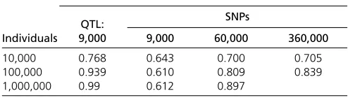
Since breeding values are of utmost importance to breeders, it is of course essential to be able to predict these breeding values correctly. In the data sets, the traits were defined by 9000 random QTL, whose effects were drawn from a normal distribution. For every animal, the QTL genotype is available and thus the true breeding value (TBV) is nothing else but the sum of the QTL effects. Table 2 presents the Pearson cor-relation between the EBVs and TBVs for different sizes of the population in the data set and different numbers of SNP markers used. Unfortunately, generating a data set of 1,000,000 individuals genotyped for 360,000 SNPs was not feasible, due to limitations of the simulation software AlphaDrop. Although the Stevin computing infrastructure includes a machine with 120 GB of working memory, it seemed that this was not sufficient to generate this large data set. Nonetheless, DAIRRy-BLUP would be able to analyze such a data set as only the read-in time would be 10 times higher compared to the analysis of the data set consisting of 100,000 individuals genotyped for 360,000 SNPs.
In the second column of Table 2, the results are listed for EBVs based on the QTL genotypes. In this case the random effects are the QTL of which it is known that they influence the phenotypic score by a predetermined effect. In the next paragraph, the estimates of the QTL effects are discussed, but here only the EBVs based on the estimated QTL effects are examined. As expected, it is confirmed that when all loci that contribute to the trait are known and genotypes for these loci are available, EBVs are always more accurate than when relying on genotypes for random SNPs. However, even when the exact positions of the QTL are known, it is ob-served that predictions of the EBVs are more accurate when the number of individuals is an order of magnitude higher than the number of QTL. The results also indicate that it is more opportune to collect genotypic and phenotypic records of more individuals than to increase the number of SNP
Table 3 Pearson correlation between the estimated QTL effects and the true QTL effects
Individuals Prediction accuracy of QTL effects
10,000 0.354
100,000 0.669
1,000,000 0.851
Table 2 Pearson correlation between the estimated breeding values (EBVs) and the true breeding values (TBVs), for data sets with different numbers of individuals and genotyped for different numbers of SNPs
Pearson correlation between TBVs and EBVs based on
QTL: SNPs
Individuals 9,000 9,000 60,000 360,000
10,000 0.768 0.643 0.700 0.705
100,000 0.939 0.610 0.809 0.839
1,000,000 0.99 0.612 0.897
markers in the genotypic records, at least when the number of markers is already sufficiently higher than the number of QTL involved. Current large-scale genomic evaluations are performed for at most 50,000 individuals genotyped for 50,000 SNPs (Gaoet al.2012; Tsurutaet al.2013), where more information is included using sparse pedigree information of nongenotyped individuals. To improve prediction accuracies of these genomic evaluations, it is shown here that instead of using denser SNP arrays, it is more interesting to increase the number of genotyped individuals.
Estimating QTL effects
Breeding values already provide a lot of information to breeders, but it is sometimes interesting to have a good estimate of the marker effects. In the simulated data sets the phenotypic scores are determined by the true QTL effects and the QTL genotypes of the individuals. True SNP marker effects are not known because SNP markers are randomly drawn and there is no information available about the linkage disequilibrium between the QTL and the SNP markers. Therefore, only the Pearson correlation between the estimated QTL effects and the true QTL effects is given in Table 3. When comparing the results of Table 3 with those in Table 2, it is seen that although the estimates of the marker effects can be quite poor, the resulting estimates of the breeding values might still be fairly accurate. Of course, when trying to identify the positions of important QTL, it is essential to have access to accurate estimates of SNP marker effects and it is observed that large numbers of genotypic and phenotypic records are then required.
Parallel efficiency
The primary motivation for the development of DAIRRy-BLUP is that it enables the analysis of large-scale data sets beyond the memory capacity of a single node. This is achieved by the distribution of all matrices and vectors involved in the model among the local memories of a large number of computing nodes. Additionally, DAIRRy-BLUP leads to a significant re-duction in runtime because the required computations are performed by several CPU cores concurrently. The parallel speedupSP is defined asSP¼T1=TP;whereTP denotes the runtime onPCPU cores. The parallel efficiencyhPis defined
as the ratio of the parallel speedup and the number of CPU
cores used: hP¼SP=P: In the ideal case, the speedupSP is equal to the number of cores used and the parallel efficiency is 100%. However, due to all sorts of overhead such as inter-process communication and load misbalance, the parallel efficiency is typically lower.
To determine the parallel efficiencyhPfor the largest
prob-lem,i.e., the data set with 100,000 individuals genotyped for 360,000 SNPs, the runtimeT1on a single CPU core is required. As it is impractical to obtain this value through a direct mea-surement, it is estimated through extrapolation of the runtime of a smaller problem with 100,000 individuals genotyped for 30,000 SNPs, taking into account the computational complex-ity of the algorithm. The dominating complexcomplex-ity is determined by the Cholesky decomposition and solution of the MMEs, which are known to have cubic complexity. However, the con-struction of the coefficient matrixCis also a time-consuming factor since it has a complexity ofO(ns2) and the number of
individuals (n) thus plays an important role when it has the same order of magnitude as the number of SNPs (s), as was the case for both data sets (n= 100,000). Therefore, the runtime for the construction of the coefficient matrix was extrapolated separately because of its quadratic complexity in the number of SNPs, as opposed to the cubic complexity of the other time-consuming parts of the algorithm.
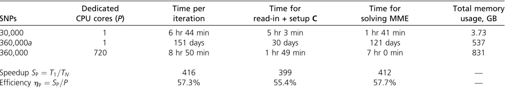
Table 4 lists the computational demands for the smaller data set with 30,000 SNPs when evaluated on a single CPU core and the estimated runtime and memory requirements for the large data set with 360,000 SNPs on a single CPU core. The timings were averaged over the required iterations, because convergence was reached in a different number of iterations for both data sets. It is clear from Table 4 that the analysis of the 360,000-SNPs data set becomes computation-ally impractical when not applying any parallel programming paradigm as the processing of the data set would require several months of computing time. By applying DAIRRy-BLUP on a cluster with 720 CPU cores, predictions of marker effects could be calculated 400 times faster. This corresponds to a parallel efficiency .55%, which is generally considered acceptable. Additionally, the memory requirements do not pose any problem, since the distributed-memory framework allows for the aggregation of the local memory (2 GB) avail-able to every CPU core, which means that a total of 1440 GB RAM could be used.
Table 4 Illustration of the parallel efficiency of DAIRRy-BLUP for a data set with 100,000 individuals genotyped for 360,000 SNPs
SNPs
Dedicated
CPU cores (P)
Time per iteration
Time for
read-in + setupC
Time for solving MME
Total memory usage, GB
30,000 1 6 hr 44 min 5 hr 3 min 1 hr 41 min 3.73
360,000a 1 151 days 30 days 121 days 537
360,000 720 8 hr 50 min 1 hr 49 min 7 hr 0 min 831
SpeedupSP¼T1=TN 416 399 412 —
EfficiencyhP¼SP=P 57.3% 55.4% 57.7% —
Speedup is calculated as the ratio between the computing time on a single CPU core and the computing time onP= 720 CPU cores. Parallel efficiency is defined as the ratio between the actual speedup and the maximum speedup, which is equal to the number of dedicated CPU cores.
aResults for a data set with 360,000 SNPs on a single CPU core are estimated based on results of the data set with 30,000 SNPs, cubic complexity of the solving algorithm,
Discussion
As has been pointed out by Coleet al.(2012), there is a need to be able to process and analyze large-scale data sets, using high-performance computing techniques. DAIRRy-BLUP, a distributed-memory computing framework for genomic prediction, is presented and meets some of the issues addressed by Cole et al. It has been shown that DAIRRy-BLUP is able to analyze large-scale genomic data sets in an efficient way when sufficient computing power is available. It is also suggested that analyzing such large-scale genomic data sets is necessary for obtaining better prediction accu-racies for marker effects and breeding values, as was already suggested by Hayes et al. (2009) and VanRaden et al.
(2009). The results show that genotyping more individuals has a stronger effect on prediction accuracy than genotyping for a higher number of SNPs, although an increasing number of SNPs can also provide a higher prediction accuracy. This effect is in accordance with the observations by Habieret al.
(2013), where a plateau was already reached for15,000 SNPs, but the phenotypes were influenced by only 200 QTL as opposed to 9000 QTL in our study. The number of indi-viduals was also quite low (maximum 2000), but an in-crease of prediction accuracy was already noticeable when increasing the number of individuals in the training data. These results, together with the results obtained with DAIRRy-BLUP, justify the choice for an algorithm whose computational demands are dominated by the number of estimated random effects rather than by the number of individuals included in the analysis.
If the exact positions of the QTL on the chromosomes are known and animals can be genotyped for these QTL, prediction accuracies might improve substantially. Additionally, if a large number of phenotypic records of QTL-genotyped individuals is present, the effects of the different QTL can be estimated with significant accuracy. Current real data sets are probably still too small to obtain an accurate estimation of the marker effects; nonetheless, as the cost of genotyping is constantly decreasing, future data sets will contain the potential for identifying QTL on a large scale.
The results of this study on simulated data sets indicate that for accurate genomic predictions of breeding values, the number of genotyped individuals included in the analysis should increase substantially. Due to the constant decrease in cost for genotyping animals or plants, it is assumed that such large-scale data sets will be available in the near future. Since analysis of these data sets on a single computing node becomes computationally impractical, DAIRRy-BLUP was developed to enable the application of a distributed-memory compute cluster for predicting EBVs based on the entire data set with a significant speedup.
Acknowledgments
The computational resources (Stevin Supercomputer Infra-structure) and services used in this work were provided by
Ghent University, the Hercules Foundation, and the Flemish Government–department EWI (Economie, Wetenschap en Innovatie). This study was funded by the Ghent University Multidisciplinary Research Partnership“Bioinformatics: from nucleotides to networks.”
Literature Cited
Blackford, L. S., J. Choi, A. Cleary, E. D’Azevedo, J. Demmelet al., 1997 ScaLAPACK Users’Guide. SIAM, Philadelphia.
Chen, G. K., P. Marjoram, and J. D. Wall, 2009 Fast andflexible simulation of DNA sequence data. Genome Res. 19: 136–142. Choi, J., J. Dongarra, S. Ostrouchov, A. Petitet, D. Walker et al.,
1996a A proposal for a set of parallel basic linear algebra subprograms, pp. 107–114 inApplied Parallel Computing Com-putations in Physics,Chemistry and Engineering Science, edited by J. Dongarra, K. Madsen, and J. Wasniewski. Springer-Verlag, Berlin/Heidelberg, Germany.
Choi, J., J. Dongarra, S. Ostrouchov, A. Petitet, D. Walkeret al., 1996b Design and implementation of the ScaLAPACK LU, QR, and Cholesky factorization routines. Sci. Program. 5: 173–184.
Cole, J. B., S. Newman, F. Foertter, I. Aguilar, and M. Coffey, 2012 Really big data: processing and analysis of very large data sets. J. Anim. Sci. 90: 723–733.
Daetwyler, H. D., M. P. L. Calus, R. Pong-Wong, G. de los Campos, and J. M. Hickey, 2013 Genomic prediction in animals and plants: simulation of data, validation, reporting, and bench-marking. Genetics 193: 347–365.
de Koning, D.-J., and L. McIntyre, 2012 Setting the standard: a special focus on genomic selection in GENETICS and G3. Genetics 190: 1151–1152.
Gao, H., O. F. Christensen, P. Madsen, U. S. Nielsen, Y. Zhanget al., 2012 Comparison on genomic predictions using three GBLUP methods and two single-step blending methods in the Nordic Holstein population. Genet. Sel. Evol. 44: 8–16.
Gilmour, A. R., R. Thompson, and B. R. Cullis, 1995 Average information REML: an efficient algorithm for variance param-eter estimation in linear mixed models. Biometrics 51: 1440– 1450.
Habier, D., R. L. Fernando, and D. J. Garrick, 2013 Genomic BLUP decoded: a look into the black box of genomic prediction. Genetics 194: 597–607.
Hayes, B., P. Bowman, A. Chamberlain, and M. Goddard, 2009 Genomic selection in dairy cattle: progress and challenges. J. Dairy Sci. 92: 433–443.
HDF Group, 2000–2010 Hierarchical data format version 5. Avail-able at: http://www.hdfgroup.org/HDF5. Accessed: April 24, 2014.
Henderson, C. R., 1963 Selection index and expected genetic ad-vance, pp. 141–163 in Statistical Genetics and Plant Breeding 982, edited by W. D. Hanson, and H. F. Robinson. National Academies Press, Washington, DC.
Hickey, J. M., and G. Gorjanc, 2012 Simulated data for genomic selection and genome-wide association studies using a combination of coalescent and gene drop methods. G32:425–427.
Legarra, A., and I. Misztal, 2008 Computing strategies in genome-wide selection. J. Dairy Sci. 91: 360–366.
Legarra, A., C. Robert-Granié, P. Croiseau, F. Guillaume, and S. Fritz, 2011 Improved Lasso for genomic selection. Genet. Res. 93: 77–87.
Meuwissen, T. H. E., B. J. Hayes, and M. E. Goddard, 2001 Prediction of total genetic value using genome-wide dense marker maps. Genetics 157: 1819–1829.
Misztal, I., S. Tsuruta, T. Strabel, B. Auvray, T. Druet et al., 2002 BLUPF90 family of programs. Available at: http://nce. ads.uga.edu/wiki/doku.php. Accessed: April 24, 2014. Misztal, I., A. Legarra, and I. Aguilar, 2009 Computing procedures
for genetic evaluation including phenotypic, full pedigree, and genomic information. J. Dairy Sci. 92: 4648–4655.
Patterson, H. D., and R. Thompson, 1971 Recovery of inter-block in-formation when block sizes are unequal. Biometrika 58: 545–554. Piepho, H. P., 2009 Ridge regression and extensions for
genome-wide selection in maize. Crop Sci. 49: 1165–1176.
Piepho, H. P., J. O. Ogutu, T. Schulz-Streeck, B. Estaghvirou, A. Gordilloet al., 2012 Efficient computation of ridge-regression best linear unbiased prediction in genomic selection in plant breeding. Crop Sci. 52: 1093–1104.
Shen, X., M. Alam, F. Fikse, and L. Rönnegård, 2013 A novel generalized ridge regression method for quantitative genetics. Genetics 193: 1255–1268.
Snir, M., S. Otto, S. Huss-Lederman, D. Walker, and J. Dongarra, 1995 MPI: The Complete Reference. MIT Press, Cambridge, MA.
Tsuruta, S., I. Misztal, and T. J. Lawlor, 2013 Short communica-tion: Genomic evaluations offinal score for US Holsteins benefit from the inclusion of genotypes on cow. J. Dairy Sci. 96: 3332– 3335.
Van De Geijn, R. A., and J. Watts, 1997 SUMMA: scalable univer-sal matrix multiplication algorithm. Concurrency Pract. Exper. 9: 255–274.
VanRaden, P. M., 2008 Efficient methods to compute genomic predictions. J. Dairy Sci. 91: 4414–4423.
VanRaden, P. M., C. V. Tassell, G. Wiggans, T. Sonstegard, R. Schnabel et al., 2009 Invited review: reliability of genomic predictions for North American Holstein bulls. J. Dairy Sci. 92: 16–24.
Wetterstrand, K. A., 2014 DNA sequencing costs: data from the NHGRI Genome Sequencing Program (GSP). Available at:
www.genome.gov/sequencingcosts. Accessed February 11, 2014.
Wimmer, V., T. Albrecht, H.-J. Auinger, and C.-C. Schön, 2012 Synbreed: a framework for the analysis of genomic pre-diction data using R. Bioinformatics 28: 2086–2087.
Communicating editor: N. Yi
Appendix
A Detailed Derivation of the AI Update Matrix
Newton’s method for maximizing a likelihood function uses the Hessian matrix to update the variance components at each iteration (Equation 2). The elements of this matrix are the second-order derivatives of the REML log-likelihood with respect to the variance components,
@2l REML
@s4e ¼ n2t
2s4e 2 yTPy
s6 e
@2l REML
@s2 e@g
¼ 2yTPVgPy
2s4 e
@2l REML
@g2 ¼
tr PVg
2
2 2
tr PVgg
2
2 y
T PV
g
2
Py s2
e
þ yTPVggPy
2s2 e
;
with Vg¼dV=dg and Vgg¼@2V=@g2: An alternative is to use the Fisher information matrix, whose elements are the expected values of the Hessian matrix:
E
@2l REML
@s4 e
¼ 2n2t
2s4 e
E
@2l REML
@s2 e@g
¼ 2tr
PVg
2s2 e
E
@2l REML
@g2
¼ 2tr PVg
2
2 :
HAI
s2e;s2e¼ 2y
TPy
2s6 e
HAI
s2e;g¼ 2y
TPV
gPy
2s4 e
HAIðg;gÞ ¼ 2y TPV
g
2
Py
2s2 e
:
To arrive at these equations, the expressions yTPV
gPy=s2e andyTPVggPy=s2e are approximated by their expected values
trðPVgÞ and trðPVggÞ: When the variance structure is linear in g and thus Vgg ¼0; HAIðg;gÞ is the exact average of
@2
lREML=@g2and Eð@2lREML=@g2Þ:
Introducing a working variateyg¼VgPy¼Z^u=g;the AI matrix can be calculated as
HAI¼ 1 2s2
e y
s2e yg
T
P
y
s2
e yg
:
Such a matrixQTPQis also the Schur complement of the coefficient matrixCin matrixM:
with
M¼ "
QTR21Q QTR21W
WTR21Q C #
;
W¼ ½X Z:
(A1)
Algorithmic Details: Distribution of Matrices Among All Processes
The distributed-memory computing approach involves splitting up large matrices into smaller blocks that are distributed among the available processes. A process is an instance of DAIRRy-BLUP that is executed on a CPU core of one of the available networked nodes. In this way every process can perform certain operations in parallel on the blocks that are at its disposal. When a certain process needs information about a block that is assigned to another process, it can receive this information through message passing over the network. To obtain maximal efficiency, it is advised to map every process on a one-to-one basis onto the available CPU cores and to set the number of processes such that neither the available amount of working memory per CPU core is superseded nor the communication between processes exceeds computation time.
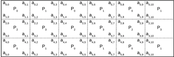
PBLAS and ScaLAPACK are libraries that can perform most essential algebraic operations on distributed matrices. They rely on a two-dimensional (2D) block cyclic distribution of matrices as is schematically depicted in Figure A1.
It is easily seen that addition of such a matrix with another matrix, distributed in the same way, can be performed in parallel on all processes without any communication overhead. The details of more complex operations performed on distributed matrices can be found in specialized literature (e.g., Choiet al.1996b; Van De Geijn and Watts 1997).
In DAIRRy-BLUP all available processes read in only their parts of the matricesXandZas illustrated in Figure A1. The matrix multiplications needed for the setup of the MME are performed in a distributed way and the resulting coefficient matrix is thus directly distributed among all available processes. The distribution of the coefficient matrix is not changed by any operation performed on the coefficient matrix.
Algorithmic Details: Calculation Flow
The calculation flow for the DAIRRy-BLUP implementation is presented here. The way matrices are distributed among processes is not explicitly mentioned since this depends on the number of processes involved and the chosen size of the blocks. The processes are always mapped to a 2D grid, where the number of columns is as close as possible to the number of rows, since this is recommended in theScaLAPACK User’s Guide(Blackfordet al.1997). Below are listed the main steps of the algorithm; the complete code can be obtained athttps://github.ugent.be/pages/ardconin/DAIRRy-BLUP/.
1. Every process reads in the blocks of matricesX,Z, andythat are assigned to it by the 2D block cyclic distribution and the coefficient matrix as well as the right-hand side of the MME is calculated using Equation 4 to obtainZTZ;XTX;XTZ;ZTy;
andXTy:Thefirst two multiplications are calculated using the level 3 PBLAS routine PDSYRK and the others using the
level 3 PBLAS routine PDGEMM.
3. Estimates for the random andfixed effects are obtained by directly solving the MME, using the Cholesky decomposition of
Cand the PDPOTRS ScaLAPACK routine. 4. An estimation fors2
e is calculated by all processes as (usingQ=yin Equation A1)
s2e ¼y
TPy
n2t¼
1
n2t
yTy2yTW ^
b ^ u
;
whereyTyis calculated as the square of the Euclidian norm ofy, obtained with the level 1 PBLAS routine PDNRM2.
5. Construct matricesXTQandZTQ, withQas defined in Equation 3, using the level 3 PBLAS routine PDGEMM, and solve
the following linear equation with the PDPOTRS ScaLAPACK routine for matrixR:
CR¼ "
XTQ
ZTQ #
:
6. The AI update matrix is calculated as the Schur complement of the coefficient matrix inside the matrixM(Equation A1), which can be calculated as
HAI¼QTPQ¼QTQ2QTWR:
7. Using the Cholesky decomposition the inverse ofCis calculated with the PDPOTRI ScaLAPACK routine and the trace of
C21is calculated with the BLACS routine DGSUM2D for obtaining the score function as defined in Equation 1.
8. As long as the relative updates fors2uand the REML log-likelihood are not smaller thane= 0.01, repeat from step 1 using
an updated value fors2
uands2e:The iterative cycle is also stopped when the maximum number of iterations is reached
(default 20). The values of e and the maximum number of iterations can be changed by the user to obtain faster convergence or more accurate solutions.
9. Optionally, breeding values can be calculated for a large-scale data set based on the estimates of the SNP marker effects. Genotypes for the test set are read in by all processes in a distributed way as defined by the 2D block cyclic distribution. To minimize memory requirements, breeding values are calculated in strips, which means that only a few breeding values are calculated in parallel by the level 3 PBLAS routine PDGEMM. The number of breeding values calculated in parallel is defined by the chosen block size and the number of dedicated processes.
Figure A1 Schematic representation of a 6311 matrix distributed among four processes, using 2D block cyclic distribu-tion with blocks of size 232.Psis the
process that holds into memory the ele-mentsai,jof the matrix, inside the small
GENETICS
Supporting Information http://www.genetics.org/lookup/suppl/doi:10.1534/genetics.114.163683/-/DC1
DAIRRy-BLUP: A High-Performance Computing
Approach to Genomic Prediction
Arne De Coninck, Jan Fostier, Steven Maenhout, and Bernard De BaetsFile S1
Input for data simulation