University of Windsor University of Windsor
Scholarship at UWindsor
Scholarship at UWindsor
Electronic Theses and Dissertations Theses, Dissertations, and Major Papers
2016
Mining Frequent Sequential Patterns From Multiple Databases
Mining Frequent Sequential Patterns From Multiple Databases
Using Transaction Ids
Using Transaction Ids
Vignesh Aravindan University of Windsor
Follow this and additional works at: https://scholar.uwindsor.ca/etd
Recommended Citation Recommended Citation
Aravindan, Vignesh, "Mining Frequent Sequential Patterns From Multiple Databases Using Transaction Ids" (2016). Electronic Theses and Dissertations. 5901.
https://scholar.uwindsor.ca/etd/5901
This online database contains the full-text of PhD dissertations and Masters’ theses of University of Windsor students from 1954 forward. These documents are made available for personal study and research purposes only, in accordance with the Canadian Copyright Act and the Creative Commons license—CC BY-NC-ND (Attribution, Non-Commercial, No Derivative Works). Under this license, works must always be attributed to the copyright holder (original author), cannot be used for any commercial purposes, and may not be altered. Any other use would require the permission of the copyright holder. Students may inquire about withdrawing their dissertation and/or thesis from this database. For additional inquiries, please contact the repository administrator via email
Mining Frequent Sequential Patterns From Multiple
Databases Using Transaction Ids
By
Vignesh Aravindan
A Thesis
Submitted to the Faculty of Graduate Studies through the School of Computer
Science in Partial Fulfillment of the Requirements for the Degree of Master of
Science at the
University of Windsor
Windsor, Ontario, Canada
2016
Mining Frequent Sequential Patterns From Multiple
Databases Using Transaction ids
By
Vignesh Aravindan
APPROVED BY:
Dr. Animesh Sarker, External Reader Department of Mathematics & Statistics
Dr. Boufama Boubakeur, Internal Reader School of Computer Science
Dr. Christie I. Ezeife, Advisor School of Computer Science
iii
DECLARATION OF ORIGINALITY
I hereby certify that I am the sole author of this thesis and that no part of this thesis has been published or
submitted for publication. I certify that, to the best of my knowledge, my thesis does not infringe upon
anyone’s copyright nor violate any proprietary rights and that any ideas, techniques, quotations, or any
other material from the work of other people included in my thesis, published or otherwise, are fully
acknowledged in accordance with the standard referencing practices.
I declare that this is a true copy of my thesis, including any final revisions, as approved by my thesis
committee and the Graduate Studies office, and that this thesis has not been submitted for a higher degree
iv ABSTRACT
Mining frequent sequential patterns from multiple databases to discover more complex patterns from multiple data sources such as multiple E-Commerce (B2C) web sites for comparative, historical and derived analysis, poses the additional challenge of integrating mined patterns from multiple sources during various levels of mining. A few existing work on mining frequent patterns from multiple databases (MDB’s) are the ApproxMap algorithm and the TidFP algorithm. The ApproxMap algorithm breaks its input sequences (e.g., the 2-column sequence <(123)(45)>) into columns so it can find the collection of approximate frequent sequences of all the columns as the approximate sequence of the database. The same method is used to integrate frequent sequences from each MDB that must have the same table structure. The TidFP algorithm mines frequent item_sets from multiple sources of different table structures and related through foreign key attributes using transaction ids for integrating patterns through set operations (e.g., intersect, union) in order to answer global queries involving multiple sources. The limitations of existing work on multiple database sequential pattern mining such as the ApproxMap algorithm is that they are not able to mine frequent sequences to answer exact and historical queries from MDB’s of different structure; while the TidFp algorithm can only answer queries from MDB’s on item_sets but not for sequences.
This thesis proposes the Transaction id frequent sequence pattern (TidFSeq) algorithm which uses the techniques of the TidFP algorithm for mining item sets on the problem of mining frequent sequences from diverse MDB’s. The challenges with mining frequent sequences from MDBs that is solved by this thesis are that the TidFSeq algorithm first computes the element (ie. Sequence item position id) in which each item in each sequence (ie. sequence id) occurs by replacing the <frequent items, transaction id list> tuple used in the TidFp with a <frequent sequences, sequence column position id list> tuple. For every item ‘i’ in the kth sequence of n-sequence of length ‘n’, the TidFSeq algorithm first transforms it into a tuple that specifies (a) it’s transaction id (Tid) and (b) the list of the kth sequence in this transaction that item ‘i’ occurs (called it’s position id list). Next the GSP-like candidate generation approach is used on our transformed sequences to generate frequent sequences with transacion ids which can be used to answer complex queries from MDB’s through set operations. The proposed TidFSeq algorithm, PrefixSpan algorithm and ApproxMap algorithm are compared with respect to the results obtained for a given query, processing speed and memory requirement. Experiments show that the proposed TidFSeq algorithm mines the exact frequent sequences (ie. 100% accuracy) from multiple sequence tables, when compared to the ApproxMap algorithm that has an accuracy of 79%. The TidFSeq algorithm has faster processing time for mining frequent sequences from multiple tables than the PrefixSpan and ApproxMap algorithms.
v
DEDICATION
This thesis is dedicated to my father Aravindan Somasundaram, Mother Suba Aravindan and my brother
Vishnuvardhan Aravindan. Without their patience, understanding, support, and most of all love, the
vi
ACKNOWLEDGEMENT
I would like to give my sincere appreciation to all of the people who have helped me throughout my education. I express my heartfelt gratitude to my parents and brother for their support throughout my graduate studies.
I am very grateful to my supervisor, Dr. Christie Ezeife for her continuous support throughout my graduate study. She always guided me and encouraged me throughout the process of this research work, taking time to read all my thesis updates and for providing financial support through research assistantship.
I would also like to thank my external reader, Dr.Animesh Sarker, my internal reader, Dr.Boufama Boubakeur, and my thesis committee chair, Dr. Ngom for making time to be in my thesis committee, reading the thesis and providing valuable input. I appreciate all your valuable suggestions and the time, which have helped improve the quality of this thesis.
vii
TABLE OF CONTENTS
DECLARATION OF ORIGINALITY ... iii
ABSTRACT ... iv
DEDICATION... v
ACKNOWLEDGEMENT ... vi
TABLE OF FIGURES………....ix
TABLE OF TABLES………...xi
CHAPTER 1: INTRODUCTION ... 1
1.1Data Mining Techniques ... 6
1.2 Existing work on mining multiple databases ... 12
1.2.1 Mining frequent patterns from multiple tables having same structure... 15
1.2.2Mining frequent patterns from multiple tables having different structure ... 16
1.4 Thesis Contributions: ... 18
1.5 Outline Of Thesis: ... 23
CHAPTER 2: RELATED WORK ... 24
2.1 Frequent itemset mining algorithms ... 24
2.1.1 Apriori algorithm ... 24
2.1.2 FP-tree Algorithm ... 26
2.2 Frequent Sequence mining algorithms ... 31
2.2.1 GSP Algorithm ... 31
2.2.2 SPAM algorithm ... 34
2.2.3 PrefixSpan algorithm ... 39
2.2.4 PLWAP algorithm ... 42
2.3 Mining frequent patterns from multiple databases ... 45
2.3.1 ApproxMap algorithm ... 45
2.3.2 TidFp Algorithm ... 49
2.3.3 Kernel estimation to identify valuable customers ... 52
2.3.4 Mining Stable patterns from multiple correlated databases ... 55
2.3.5 Identifying relevant databases ... 58
viii
2.3.7 Clustering local frequent items in multiple databases ... 63
CHAPTER 3 : PROPOSED TIDFSEQ ALGORITHM ... 65
3.1Problems Addressed ... 68
3.2 Definitions used in proposed algorithm ... 68
3.3The TidFseq Algorithm ... 69
3.4 Example Application of TidFSeq Algorithm ... 75
3.5Flowchart for TidFSeq algorithm ... 83
CHAPTER 4: EVALUATION OF TIDFSEQ ALGORITHM ... 87
4.1 Comparison of algorithms over the query handled... 87
4.2 Comparison of execution speed (speed of processing) of the algorithms ... 90
4.2.1 Execution times (in secs) for different datasets of different sizes at MinSupport of 40% ... 90
4.2.2 Execution times (in secs) for small-sized dataset (250K) for different support counts ... 91
4.2.3 Execution times (in secs) for Medium-sized dataset (500K) for different support counts ... 92
4.2.4 Execution times for large-sized dataset (2M) for different support count. ... 93
4.2.5 Memory Usages (in terms of MB) for Different Data Sizes at Minsupport of 40% ... 93
4.3 Comparison of algorithms based on Acuracy of the frequent sequences obtained for datasets of different sizes ... 95
4.3.1 Acuracy of the frequent sequences obtained for datasets conatining 250K, 500K, 750K sequences at Minsupport of 40%. ... 95
4.4 Comparison of algorithms based on execution speed for (250K) dataset having longer sequences at Minsupport of 20% . ... 95
CHAPTER 5: CONCLUSION AND FUTURE WORK... 97
5.1 Future Work ... 97
REFERENCES ... 98
ix
TABLE OF FIGURES
Figure 1: Classification dataset………07
Figure 2: Decision tree………...……….………..08
Figure 3: Clustering Dataset……….……….….……….09
Figure 4: Initial clusters…...……….……….….……….09
Figure 5: Grouping data into clusters…………...……….……….…10
Figure 6: Local branch sequence databases having same structure ………..…….13
Figure 7: Attribute relationship for local branch sequence databases having same structure..13
Figure 8: Attribute relationship for sequence databases having different structure...…..……14
Figure 9: Constucrtion Fp-tree……….………..……….……..29
Figure 10: Final frequent sequences……….…..…34
Figure 11: Vertical Bitmap of items in transaction db……….36
Figure 12: Lexicographic tree……….…...37
Figure 13: S-step………..………..…...38
Figure 14: I-step………38
Figure 15: PrefixSpan algorithm………..………41
Figure 16: Construction of PLWAP tree………..………...44
Figure 17: Support Counts of Candidate Items in Each Sequence Column………47
Figure 18: Local databases………...53
x
Figure 20: Database 2………....59
Figure 21: RF values of Db1……….….61
Figure 22: RF values of Db2……….….61
Figure 23: Multiple databases (Db1, Db2)……….………...62
Figure 24: local db1 and local db2………..………. 62
Figure 25: TidFSeq Algorithm……….………..70
Figure 26: I-step pruning ()……….….………..72
Figure 27: S-step pruning ()……….……….……….74
Figure 28 (a)(b): Final output for TidFSeq algorithm……….……..……..82
Figure 29: Proposed system flowdiagram……….………84
Figure 30: Input 1……….………..…….87
Figure 31: Input 2………..……..87
Figure 32: Execution times for different datasets of different sizes at MinSupport of 40%...90
Figure 33: Execution times (in secs) for small-sized dataset (250K) for different support counts..91
Figure 34: Execution times (in secs) for Medium-sized dataset (500K) for different support counts……….………...92
Figure 35: Execution times (in secs) for large-sized dataset (2M) for different support counts………93
xi
TABLE OF TABLES
Table 1: Transaction table………. 11
Table 2: Sequence Table……… 12
Table 3: Customer/sequence of items purchased……….………14
Table 4: Discounts / sequence of customers who avail it……….……14
Table 5: Summary of existing systems in multiple database mining...19
Table 6: Transaction db………..……….…...25
Table 7: Transaction db………..28
Table 8: Transaction db sorted according to descending order of support counts………...28
Table 9: Final result………...……….………30
Table 10: GSP sequence table………..………..32
Table 11: Frequent-1 items……….………...32
Table 12: Candidate sequences gnerated using GSP-gen join…….………...33
Table 13: Spam transaction db………..……...……….35
Table 14: Web access sequence database………..………..………..43
Table 15: Windsor branch sequence table………..…………..………....46
Table 16: Hamilton branch sequence table………..………….………....46
Table 17: Preprocessed Windsor table……….………...……..46
Table 18: Preprocessed Hamilton table………..………..47
Table 19: Finding global approximate patterns………...48
Table 20: Transaction Table Drug/Side-effect………..………...50
Table 21: Transaction Table Patient/Drug………..……….…....50
Table 22: Transaction table 1………..……….……..55
Table 23: Transaction table 2……….………56
Table 24: Drug/side-effects………....……….……76
xii
Table 26: Transformed 1-candidate item sequences for MDB1……….……….77
Table 27: Transformed 1-candidate item sequences for MDB2………..………....77
Table 28: Comparison of query handling done by TidFSeq, ApproxMap and
PrefixSpan algorithms……….………..……..89 Table 29: Execution times (in secs) for different datasets of different sizes at
MinSupport of 40%...90 Table 30: Execution times (in secs) for small-sized dataset (250K) for different
support counts………..……….…..91 Table 31: Execution times (in secs) for Medium-sized dataset (500K) for different
support counts………..………...92 Table 32: Execution times for large-sized dataset (2M) for different support counts……..……....93 Table 33: Memory Usages for Different Data Sizes at Minsupport of 40%...94 Table 34: Acuracy of the frequent sequences obtained for datasets conatining 250K,
1
CHAPTER 1: INTRODUCTION
2
But these single sequence/itemset database mining algorithms cannot mine frequent patterns from multiple databases such as Drug/side-effects sequence table and Patient/Drug sequence table and integrate the results such that it can answer queries related to multiple databases. For example, for multiple related sequence tables, such as Drug/side-effects sequence table and Patient/Drug sequence table, a standard frequent sequence mining algorithm such as GSP (Srikant and Agrawal (1996)) will only mine the frequent sequence of side-effects from Drug/Side effects sequence table and mine the frequent sequence of drugs purchased from Patient/Drugs sequence table, the final set of frequent sequences obtained from each sequence table cannot be used to answer queries such as, find the frequent sequence of side effects that patients p1 and p3 suffer from. Some of the reasons for the need to mine frequent patterns from multiple databases and the example queries for each category is listed below:
1) Comparative analysis: In applications such as E-Commerce sites, the information of products (such as product name, price) sold by each online store (such as Bestbuy) are constantly stored in multiple databases. For example, the laptop products sold in Bestbuy and Walmart are stored in two product databases corresponding to Bestbuy and Walmart respectively. By mining such multiple databases, apart from answering historical queries, comparative queries can also be answered, such as:
Find the E-commerce websites, from the product information tables of all the E-commerce websites that sell ‘Apple’ products with discount.
Find the set of frequently bought laptop product names from the product information tables corresponding to the E-commerce websites that provide highest discounts.
Find the E-commerce website which sells the cheapest ‘samsung’ TV products.
3
store (such as Walmart having many local branches) can be answered using the local and global frequent patterns of prodcut purchased, such as:
Find the global frequent patterns that consist of milk products in them.
Find the frequent local product patterns that are also frequent on global scale.
Find the frequent pattern of products purchased in branches located in the western region of US.
3) Mining frequent patterns from multiple tables with different structures: Not all multiple tables have the same structure, there is also a need to mine frequent itemsets/sequences from multiple related databases having different structure (ie. Patient/Drugs and Drugs/side-effects that are related by the foreign/primary key attribute: Drugs) to answer queries related to the multiple tables. For example, in an application having related sequence databases such as Patient/Drugs and Drugs/side-effects sequence databases, the mined patterns from the related sequence tables can help answer queries such as:
Find the frequent sequence of side effects that patients p1 and p3 suffer from.
Find all the patients that are affected by frequent sequence of side effects that have side effect ‘s1’ in their pattern.
4) Mining alternate types of information: Patterns such as stable patterns, finding important customers in a retail store are alternate types of information that help find useful information such as the set of standard and stable products found in all the local branches of a retail store like walmart. Example query can be answered by mining such alternate information such as:
Find the set of stable patterns from all the local branches.
Find the important customers that come to the retail store
Find the local frequent products that are similar to each other. Mining frequent patterns from multiple databases is of two types:
4
customer id and the products purchased by the customer in each of its local database)
2) Mining frequent patterns from multiple tables having different structure (for eg, Patient/Drugs and Drugs/side-effects that are related by the foreign/primary key attribute: Drugs).
Some existing systems that mine frequent patterns from multiple databases having same structure are:
1) ApproxMAP algorithm by Hyue and et al. (2006), the ApproxMap algorithm breaks its input sequences (e.g., the 2-column sequence < (123) (45) >) into columns so it can find the collection of approximate frequent sequences of all the columns as the approximate sequence of the database. The same method is applied on the local frequent sequences obtained from each local cutomer transaction database that must have the same table structure, to get the frequent global approximate sequence patterns. The main limitation of this algorithm is that it does not generate exact frequent sequence patterns and does not work for multiple tables with different structure.
2) The hierarchial Gray clustering algorithm by Yaojin and et al (2013), introduced a new concept of stable patterns. It defines an item ‘a’ as stable, if the item satisfies the minimum support count ‘s’ in each of the local transaction table (T1,T2..TN, where Ti, 1<=i<=N, is a local transaction table) that it occurs and also the variation of the support count of that item ‘a’ is less than or equal to a user defined variation value ‘v’. The algorithm clusters stable items found from multiple transaction tables into stable patterns according to the similarity of their timestamps (ie. the time at which the stable item ‘a’ was purchased by a cutomer). The use of stable patterns helps us to identify the standard set of constantly purchased items on a global scale in a retail store having local branches. Since this algorithm is specific to mining stable patterns, it is not useful to mine frequent sequences from multiple tables with different structures.
5
purchase high value products from the store) from a retail store having local branches. The local databases contain cutomer information, such as the expenditure of the customer in that local branch and the number of visits and transactions made by the customer in that local branch. Using this information the kernel estimation algorithm uses a mathematic approach to first find the local importance of each customer to the local branch. And then the global importance of the customer to the retail store. Since this algorithm is specific to mining local and global important customers, it is not useful to mine frequent sequences from multiple tables with different structures.
4) The pipeline feedback technique by Adhikari.A et al (2010) aims to give an efficient methodology to mining large sets of local databases. The main concept is to sort the databases based on decreasing order of their sizes and then mine each database using a standard frequent itemset mining algorithm such as FP tree algorithm (Han et al (2001)) and finally synthesize the large collection of patterns obtained. This technique was proposed to make the process of mining frequent itemsets from large sets of multiple transaction databases having same structure faster and is not useful to mine frequent patterns from multiple related databases. 5) Clustering local frequency items in multiple databases by Animesh.A (2013), gives
a similarity measure that is derived from the common items/products in multiple databases (for example, milk product is common item in local transaction tables corresponding to the local branches of a retail store), to cluster the frequent itemsets obtained in each local database into groups based on similarity of the frequent itemsets (for example, frequent itemsets (Ice cream, Milk) and (Milkshake, cheese) belong to same group, since all are milk based products). This method is useful to find the groups of similar frequent items in each local branch of a retail store, but it is not designed to mine frequent sequences from multiple tables with different structures.
6
1) In some application areas where there is a very large set of databases and the user needs to find specific databases from the entire set of databases, in order to query specific information, there is a need to first find the specific databases that can be queried later, to find information that the user is looking for. For example, if the query is to find the eating habits of people belonging to Sri Lanka and we are given a huge dataset of 1000 databases, then we must first find the relavant databases that can be queried to find the answer. One prominent existing work to solve this type of problem was given by Liu, Lu and Yao (2001) (belongs to category 2). They introduced a mathematical factor known as relevance factor, which identifies how close the attribute in a database is to the given query. For example, if the query is find the eating habits of people belonging to Sri Lanka and the database being checked has attributes ‘habits’ and ‘Country’, the relevance factor will be high for that database (close to 1), meaning this database can be chosen to be queried in order to find the answer for the input query. Since this paper is focused on finding the relevant databases that needs to be mined rather than mining the frequent patterns from the multiple databases, it cannot mine frequent sequences from multiple tables with different structures.
2) TidFP algorithm by Ezeife and Zhang (2009).The TidFp algorithm mines frequent item_sets from multiple sources using transaction ids for integrating patterns through set operations (e.g., intersect, union) in order to answer global queries involving multiple sources. But the main limitation is that it only mines frequent itemsets from multiple transaction tables and not frequent sequences.
It is clear that none of the existing systems are able to mine multiple related sequence tables having different structure for frequent sequences and answer queries using the result sets. The main purpose of this thesis is to develop a multiple related sequence database mining algorithm to mine the frequent sequence patterns and answer valuable user queries.
1.1 Data Mining Techniques
In this section, the three main techniques of data mining are discussed. Data mining uses three techniques, Classification, Clustering and Association rule mining.
7
The goal of classification is to accurately predict the target class for each case in the data. For example, a classification model could be used to identify loan applicants as low, medium, or high credit risks. Classification involves a training data and a test data. In the training data, the target class is known and in the test data the target class in not known. A classification algorithm finds the relationship between the target class and the predictors (ie. the rest of the attributes in the dataset) to find the value of the target class. This relationship is known as a classification model. Some prominent classification algorithms are Naive Bayes algorithm (Russell and Norvig (1995)), k-nearset neighbour algorithm (Altman (1992)). The training dataset is used to find the best classification algorithm that provides the best classification model to predict the known target class values with good accuracy. Then the same classification model is applied on the test data having unknown target class values, to check for its prediction accuracy. Figure 1 shows a classification dataset. The goal is to predict which of the customer ids (case id) are likely to increase spending if given an affinity card (target class attribute). The target class attribute affinity_card has two values ‘0’ (customer does not increase spending) and ‘1’ (customer does increase spending). The dataset is split into training dataset and test dataset. An efficient classification model (ie. the relationship between the predicates (cust_gender,education,occupation,age) and the affinity card (target class attribute)) is found for the training set and the same model is applied on the test set to predict the values for the target class attribute in test set with efficient accuracy.
Cust_id gender Age occupation education Affinity_card
1 M 20 Clerk Bach 1
2 M 21 IT Masters 1
3 F 33 IT Bach 0
4 F 22 Doctor Bach 0
Figure 1: Classification dataset
8
is either ‘Bachelors’ or ‘Masters’ and the gender of the customer is Male, the value of target class attribute (ie. affinity_card) is 1, else if the conditions are not met, value is ‘0’.
Figure 2: Decision tree
Such a classification model is learned from historical data and the rules from it are used to predict the affinity_card of incoming customers.
Clustering:
9
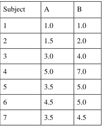
Subject A B
1 1.0 1.0
2 1.5 2.0
3 3.0 4.0
4 5.0 7.0
5 3.5 5.0
6 4.5 5.0
7 3.5 4.5
Figure 3: Clustering Dataset
The first step is to find the initial clusters. The initial clusters are taken as minimum (A, B) pair values and maximum (A, B) pair values from Figure 3. (ie. (1.0, 1.0) and (5.0, 7.0)) in our example. In our example, the initial clusters will be (1.0, 1.0) and (5.0, 7.0), belonging to individuals 1 and 4 respectively, which is shown in (Figure 4):
Individual Mean Vector(Centroid) Group 1 1 (1.0,1.0)
Group 2 4 (5.0,7.0)
Figure 4: Initial clusters
10
The formula for eucladiean distance between (A, B) value of each indivdual and (X, Y) value of the mean vector of the cluster is:
sqrt ((B-A)^2 + (Y-X)^2). This leads to a series of steps (shown in Figure 5), until every individual is assigned to a cluster that has the most similarity to the individual.
Cluster 1 Cluster 2
Step individual Mean Vector(centroid) Individual Mean Vector(centroid)
1 1 (1.0,1.0) 4 (5.0,7.0)
2 1,2 (1.2,1.5) 4 (5.0,7.0)
3 1,2,3 (1.8,2.3) 4 (5.0,7.0)
4 1,2,3 (1.8,2.3) 4,5 (4.2,6.0)
5 1,2,3 (1.8,2.3) 4,5,6 (4.3,5.7)
6 1,2,3 (1.8,2.3) 4,5,6,7 (4.1,5.4)
Figure 5: Grouping data into Clusters
Individuals 1, 2, 3 belong to cluster 1 and 4, 5, 6, 7 belong to cluster 2. Hence, from the example we can see that, items which are similar to each other are clustered together by using clustering algorithms such as K-means clustering algorithm.
Association Rule mining:
11
Table 1: Transaction table
Table 1 shows a customer transaction table of a retail store, where there are 4 transaction ids (10, 20, 30, 40) and their corresponding itemsets (items that are purchased together). For example, in TID 10, itemset (Bread, Milk) consists of items Bread and milk that are purchased together. Support of an itemset (i) = (number of occurences of i) / (number of database transactions). In example database Table 1 support of item Bread (i.e.) supp (Bread) = 3/4, since it occurs in three out of a total of four transactions. Confidence of an itemset (i) = (number of occurences of i) / (number of occurence of the antecedent of the itemset). For example, in Table 1, it can be seen that itemset (Bread, Milk) appears ‘2’ times and antecedent item -Bread appears ‘3’ times. Thus, confidence of (Bread->Milk) = 2/3. Hence, given a set of transactions T, the goal of association rule mining is to first find all the frequent itemsets having support greater than or equal to a user defined minimum support count. From the computed frequent itemsets, only strong association rules with support greater than or equal to a given minimum confidence threshold are retained. For example, if the minimum support threshold is 0.5 and minimum confidence threshold is 0.5. The association rule, >Milk is a strong association rule in Table 1, since Bread->Milk has a support of 0.5, which is greater than minimum support threshold and confidence of 0.6, which is greater than minimum confidence threshold. Table 1 shows a transaction table from which frequent itemsets can be mined using algorithms such as the Apriori algorithm (Agrawal and Srikant (1994)) and Fp-tree algorithm (Pei and et al. (2001)). Table 2 shows an example of a customer purchase sequence table, having candidate items: a, b, c and d.
TID Items purchased
10 Bread,Milk
12
CID Customer purchase sequences 1 <bcbd>
2 <ac(abc)> 3 <(abc)ac> 4 <abc>
Table 2: Sequence Table
In Table 2, each customer id (1, 2, 3, 4) is associated with a sequence of products/items purchased by the customer (cid), for example in Table 2, cid 2 consists of sequence <ac (abc)>, meaning items a, c and itemset (abc) are purchased separately at different times by the customer ‘cid 2’. Using a sequence table, frequent sequences can be generated using algorithms such as: GSP (Srikant and Agrawal (1996)), SPADE (Zaki (2001)), SPAM (Ayres and et al.(2002)), Prefix-span (Pei and et al.(2004)), PLWAP-tree algorithm (Ezeife and Lu 2005).
1.2 Existing work on mining multiple databases
Existing systems in mining frequent patterns from multiple databases can be categorized into:
13
Local branch: London db Local branch: Hamilton db Figure 6: Local branch sequence databases having same structure
Figure 7: Attribute relationship for local branch sequence databases having same
structure
2) Mining frequent patterns from multiple tables having different structure:
Patient/Drugs and Drugs/side-effects that are related by the foreign/primary key attribute: Drugs, is an example of this type. For example, Table 3 (Customer/Sequence of items purchased by the customer) and Table 4 (Discounts/sequence of customers who use the discounts) are two sequence tables which are related through the customer attribute. Figure 8 shows attribute relationship between Table 3 and Table 4. In Table 3, the customer attribute is primary/foreign key and in Table 4, Discounts attribute is primary key and Customers attribute is foreign key.
Customer_id Product_purchase_sequences
1 <(123) (1)>
2 <(123)>
3 <(3) (4)>
4 <(1) (3)>
Customer_id Product_purchase_sequences
10 <(123)>
20 <(3) (4)>
30 <(1 2) (1) (3)>
40 <(1) (3)>
Customer_id
PK
Product_purchase_sequences
FK
Customer_id
PK
Product_purchase_sequences
FK Local branch: London Table
14
Customers Sequence of items C1 <(1 2 3)>
C2 <(1) (3)> C3 <(1 2 3)> C4 <(2) (3)>
Table 3: Customer/sequence of items purchased
Table 4: Discounts / sequence of customers who avail it
Figure 8: Attribute relationship for sequence databases having different structure
The following subsections describe the related systems that belong to the above two categories of mining multiple databases, their application area in that category and their limitations.
Discounts Customers D1 <(C1) (C4)> D2 <(C1 C2 C3)> D3 <(C1 C2 C3) (C3)> D4 <(C2) (C3)>
Customers PK/FK
Sequence of items
Discounts PK
Customers FK
Table 5: Customer/sequence
of items purchased
Table 6: Discounts /
sequence of customers who
15
1.2.1 Mining frequent patterns from multiple tables having same structure
Mining the local customer transaction tables that are of the same structure (ie. having the same attributes customer_id and items_purchased in all the local customer transaction databases), will only give the frequent purchases made at each branch of a store. But mining the set of local frequent patterns (frequent itemsets or frequent sequences) will give us global frequent product purchase patterns, that help the store to assess the global impact of their products and find the most sought after products on a global scale. Some existing work related to this type of mining is ApproxMAP algorithm by Hyue and et al. (2006). The ApproxMap algorithm finds approximate frequent sequences from multiple customer purchase sequence databases, where each local database corresponds to the local branch of a retail store (eg. Windsor branch of Walmart). It breaks its input sequences (e.g., the 2-column sequence < (123) (45) >) into 2-columns so it can find the collection of approximate frequent sequences of all the columns as the approximate sequence of the database. The same method is applied on the local frequent sequences obtained from each local cutomer transaction database that must have the same table structure, to get the frequent global approximate sequence patterns. The main limitation of this algorithm is that it does not generate exact frequent sequence patterns, that will be gnerated by a standard frequent sequence mining algorithm such as GSP (Srikant and Agrawal (1996)) for a single sequence table. And also the ApproxMap algorithm does not work for multiple tables with different structure.
16
this algorithm is specific to mining stable patterns, it is not useful to mine frequent sequences from multiple tables with different structures.
The kernel estimation algorithm (belongs to category 1) by Zhang and et al (2009), introduced the concept of generating the local and global important cutomers (ie. customers who regularly purchase high value products from the store) to a retail store having local branches. This algorithm makes the assumption that a customer ‘A’ visting local branch X will also visit local branch Y. The local databases contain cutomer information, such as the expenditure of the customer in that local branch and the number of visits and transactions made by the customer in that local branch. Using this information the kernel estimation algorithm uses a mathematic approach to first find the local importance of each customer to the local branch. And then the global importance of the customer to the retail store. Since this algorithm is specific to mining local and global important customers, it is not useful to mine frequent sequences from multiple tables with different structures.
Clustering local frequency items in multiple databases by Animesh.A (2013), gives a similarity measure that is derived from the common items/products in multiple databases (for example, milk product is common item in local transaction tables corresponding to the local branches of a retail store), to cluster the frequent itemsets obtained in each local database into groups based on similarity of the frequent itemsets (for example, frequent itemsets (Ice cream, Milk) and (Milkshake, cheese) belong to same group, since all are milk based products). This method is useful to find the groups of similar frequent items in each local branch of a retail store, but it is not designed to mine frequent sequences from multiple tables with different structures.
1.2.2Mining frequent patterns from multiple tables having different structure
17
(belongs to category 2). They introduced a mathematical factor known as relevance factor, which identifies how close the attribute in a database is to the given query. For example, if the query is find the eating habits of people belonging to Sri Lanka and the database being checked has attributes ‘habits’ and ‘Country’, the relevance factor will be high for that database (close to 1), meaning this database can be chosen to be queried in order to find the answer for the input query. Since this paper is focused on finding the relevant databases that needs to be mined rather than mining the frequent patterns from the multiple databases, it cannot mine frequent sequences from multiple tables with different structures.
18 1.4 Thesis Contributions:
19
Table 5: Summary of existing systems in multiple database mining
Existing System
Technique used It’s application Limitation
ApproxMap algorithm by Hyue and et al. (2006)
Breaks its input sequences into columns so it can find the collection of approximate frequent sequences of all the columns as the approximate sequence of the database. The same method is applied on the local frequent sequences obtained from each local cutomer transaction database that must have the same table structure, to get the frequent global approximate sequence patterns.
Give the global frequent product purchase patterns of a Retail store such as Walmart, that help the store to assess the global impact of their products and find the most sought after products on a global scale
Does not generate exact frequent sequence patterns and does not answer queries for multiple related sequence tables. The hierarchial Gray clustering algorithm by Yaojin and et al (2013)
Introduces a new concept of stable patterns, it defines an item ‘a’ as stable, if the item satisfies the minimum support count ‘s’ in each of the local transaction table that it occurs and also the variation of the support count of that item ‘a’ is less than or equal to a user defined variation value ‘v’. The algorithm clusters stable items found from multiple transaction tables into stable patterns according to the similarity of their timestamps (ie. the time at which the stable item ‘a’ was purchased by a cutomer).
Helps us to identify the standard set of constantly
purchased items on a global scale in a retail store having local branches. Example:
Milk, Eggs, Cereals is a stable pattern, since it is bought by most people on a regular basis in all local branches of a retail store.
Since this algorithm is specific to mining stable patterns, it is not useful to mine frequent sequences from multiple related tables.
Clustering local frequency items in multiple databases by Animesh.A (2013)
Gives a similarity measure that is derived from the common items/products in multiple databases (for example, milk product is common item in local transaction tables corresponding to the local branches of a retail store), to cluster the frequent itemsets obtained in each local database into groups based on similarity of the frequent itemsets (for example, frequent itemsets (Ice cream, Milk) and (Milkshake, cheese) belong to same group, since all are milk based products).
This method is useful to find the groups of similar frequent items in each local branch of a retail store.
Algorithm is not designed to mine frequent sequences from multiple related tables.
The kernel estimation algorithm by Zhang and et al (2009)
Finds locally and globally important customers using kernel estimation that finds the customer lifetime value on local and global scale.
Finds customers who regularly purchase high value products from the store.
It is specific to finding the importance of the customers and not suited to find sequential patterns from MDB’s.
TidFP algorithm by Ezeife and Zhang (2009)
The TidFp algorithm mines frequent item_sets from multiple sources using transaction ids for integrating patterns through set operations (e.g., intersect, union) in order to answer global queries involving multiple sources.
Answers queries from multiple related transaction tables.
20
Problem Definition: Given multiple related sequence tables where each table consists of sequence id and corresponding sequence of items and a minimum support count ‘s’, the problem of mining frequent sequences from multiple related sequence databases is to mine the exact frequent sequences with support counts greater or equal to the given minimum support count ‘s’ from each sequence table to be able to answer complex queries on the multiple related sequence tables. For example, what are the frequent side effects that affect the patients p1 and p3? , is a query that can be answered by the proposed algorithm from Patient/sequence of drugs table and Drug/sequence of side effects table.
Feature contributions:
The following are the thesis features:
1. Mining frequent sequences from multiple related sequence databases having different structure as well as from multiple related sequence database having
similar structure for comparative mining: The problem of answering complex sequence database queries involving related data from more than one table or database is solved. Example query that can be answered is “Find the discounts associated with frequent sequence of customers in the all named retail stores”. 2. Finding records that are related to frequent sequences in multiple databases
21
3. Mining alternate types of information from competitive databases: Patterns such as stable patterns and their customers, frequent, trending patterns and their customers in a retail store can be a tool for finding important customers to be targetted for attrition by a competitive retail store as alternate types of information to advance competitor’s business. Example queries that can be answered by mining such alternate information include:
Find the set of stable patterns from all the local branches.
Find the important customers that come to the retail store.
Find the local frequent products that are similar to each other.
Procedure contributions:
This thesis solves the unsolved problems identified in the feature contribution section above by proposing the following solutions.
1. To solve the problem of mining from multiple databases with similar or different schema structures in order to answer more complex sequence queries, this thesis proposes the an algorithm called the Transaction id frequent sequence pattern (TidFSeq) algorithm for mining frequent sequences from multiple related sequence databases having similar or different structures. The candidate item sets, multiple related sequence tables and minimum support count are used as input to the proposed algorithm. The thesis algorithm is an extension of the TidFP algorithm (Ezeife and Zhang (2009)) for mining frequent itemsets from multiple tables, which now mines frequent sequences from multiple tables using an extension of the ApproxMap sequential pattern algorithm (Hyue and et al. (2006)) for mining sequential patterns from only multiple tables having similar table schemas. While the TidFP and the
ApproxMap algorithm approaches are used to pre-process and compute the format of the
fequent sequences with transaction ids found, the ApproxMap approach for finding only
22
purchased during different transactions) were termed as S-step sequences by the SPAM algorithm (Ayres and et al (2002)). The definitions of I-step sequences and S-step sequences are used in the thesis algorithm. Thus, the main six steps of the proposed TidFSeq algorithm are:
I. Linking the frequent sequences to their Database transaction record ids:
This is done by replacing the <frequent items, transaction id list> tuple used in the TidFp (Ezeife and Zhang (2009)) with a <sequence id, position id list> tuple. Each <sequence id, position id list > tuple consists of the sequence id and the sequence id attribute position of the items (sequences).
II. Find the frequent k sequences for k=1: Count the support of the candidate items from step 1 above, as the number of sequence ids in the position list. Then, keep the items with support greater or equal to minimum support as the frequent items.
III. Find the k+1 candidate sequences: This is done by joining the Fk frequent
sequences by Fk frequent sequences using GSP_gen join approach, if the
k+1 candidate sequence is not an empty set. If k+1 candidate sequence is an empty set, algorithm terminates and jumps to step VI.
IV. Find the frequent k+1 sequences for k>1: If the candidate k sequences is
not an empty set, then the following steps are used:
1) If the candidate sequence is of the I-step form of (ab) which is single item sequence then, the following conditions,condition 1: items ‘a’ and ‘b’ have same sequence ids and condition 2: the positions ids corresponding to the sequence ids are same, must be satisfied. If the number of times both the conditions are satisifed is greater or equal to min-support count, then the single item sequence of form (ab) is frequent.
23
times both the conditions are satisifed is greater or equal to min-support count, then the multi set sequence of form (a)(b) is frequent.
V. Continue finding higher order frequent sequences: Go to step 3, to continue finding all frequent sequences with longer items until either the candidate set generation step or frequent sequence generation step yields an empty set.
VI. Collect all found frequent sequences (FP): This is done as the union of all F1 to Fn, ie. the frequent sequences found so far.
2) The proposed algorithm uses the concept of <sequence id, position_id list> tuple for each frequent sequence, which enables to store the sequence ids in which the candidate sequences occur inside the <sequence id, position_id list> tuple, while the algorithm checks if the candidate sequence is frequent or not. This helps to avoid the costly method of first finding the frequent sequences and then mapping it to the corresponding sequence ids. Thus finding the frequent sequences along with their corresponding sequence ids in parallel, helps in finding records that are related to frequent sequences faster.
1.5 Outline Of Thesis:
24
CHAPTER 2: RELATED WORK
2.1 Frequent itemset mining algorithms
2.1.1 Apriori algorithm
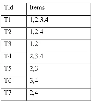
The Aprori algorithm was introduced by Agrawal and Srikant (1994). The Apriori algorithm follows the Apriori principle: An itemset is frequent only if all of its sub-itemsets are frequent. The input to the algorithm is a transaction database, the user defined support count and the candidate-1 set of items. In the first step, the support counts of each item in the candidate-1 set is calculated. All the items that satisfy the minimum support count are retained and those that do not satisfy the minimum support count are pruned (ie. removed). The items that are retained form the frequent 1 (F1) set of items. Next step is to find the candidate 2 set from the frequent 1 set using the Apriori join method. The Apriori gen-join is a self gen-join of the F1 items with itself, where an item in the F1 set is gen-joined only with the items that come after it in the F1 set (eg. {a,b,c} ap-gen join {a,b,c} is (a,b) (a,c) (b,c), c is not joined with the previous items ‘a’ and ‘b’ in the F1 set, since candidate itemsets (a,c) and (b,c) are same as (c,a) and (c,b) ). Once, the (C2) candidate-2 itemsets are generated, the frequent-2 set is generated by pruning the infrequent candidate-2 itemsets as explained above. This process of genrating candidate sets and finding frequent sets from it keep continuing until there are no more candidate sets that can be generated. The working of the Apriori algorithm is shown through an example:
25
Table 6: Transaction db
Step 1: Find frequent-1 items
The first step of Apriori is to count up the number of occurrences, called the support, of each item in the Candidate set (C1) separately, by scanning the database a first time. All the items that have support count greater than or equal to the input support count (ie. 3) are frequent items and are retained. The items that do not meet the minimum support count are pruned. The frequent 1 items in our example are: 1, 2, 3, 4.
Step 2: Candidate-2 itemset generation
The next step is to generate candidate-2 itemsets. Candidate itemsets (C2) are generated by doing Apriori-gen join of frequent 1 items (L1) with itself. The Apriori gen-join is a self join of the F1 items with itself, where an item in the F1 set is joined only with the items that come after it in the F1 set (eg. {a,b,c} ap-gen join {a,b,c} is (a,b) (a,c) (b,c), c is not joined with the previous items ‘a’ and ‘b’ in the F1 set, since candidate itemsets (a,c) and (b,c) are same as (c,a) and (c,b) ). For example, apriori-gen join of frequent 1 items found in step 1 is:
C2={1,2},{1,3},{1,4},{2,3},{2,4},{3,4} Step 3: Finding frequent-2 itemsets
From the set of candidate -2 itemsets obtained in the previous step, we can see that the pairs {1, 2}, {2, 3}, {2, 4}, and {3, 4} all meet or exceed the minimum support of 3, so
26
they are frequent. The pairs {1, 3} and {1, 4} are not, hence they are pruned. The frequent 2 itemsets for our example will be:
F2: frequent 2 itemsets = {1, 2}, {2, 3}, {2, 4}, and {3, 4}
Next, the candidate-3 itemsets are generated from the frequent-2 itemsets. The C3 set obtained by doing ap-gen join of F2 with itself is: {1,2,3} {1,2,4} {2,3,4}. Since none of the candidate-3 itemsets satisfy the minimum support count, there will be no frequent-3 itemsets. Since no more candidate itemsets can be generated, the Apriori algorithm stops. The final fequent itemset list is the union of all the frequent itemssets found so far: F=F1 U F2 = 1, 2, 3, 4, {1, 2}, {2, 3}, {2, 4}, {3, 4}.
Key features and shortcomings:
Candidate generation generates large numbers of subsets (the algorithm attempts to load up the candidate set with as many as possible before each scan). Apriori algorithm has slow processing times for huge datasets.
2.1.2 FP-tree Algorithm
The FP-Growth Algorithm, proposed by Pei and et al (2001) finds frequent itemsets without any candidate generation. It uses a tree structure known as the FP- growth tree, to compute the frequent itemsets. The input to the algorithm is a transaction database, the user defined support count and the candidate-1 set of items. In the first step, the support counts of each item in the candidate-1 set is calculated. All the items that satisfy the minimum support count are retained and those that do not satisfy the minimum support count are pruned (ie. removed). The items that are retained form the frequent 1 (F1) set of items. The set of frequent-1 items are sorted in the descending order of their support counts. And each itemset corresponding to the transaction id is ordered according to the descending order of their support counts. Next step is to construct the FP tree. An FP-tree is then constructed as follows. First, create the root of the tree, labeled with “null.”
27
(I2, I1, I5), leads to the construction of the first branch of the tree with three nodes (where each node has a corresponding count specifying number of occurences of the node in the fp-tree), I2:1, I1:1, I5:1, where I2 is linked as a child to the root, I1 is linked to I2, and I5 is linked to I1. And then if the second transaction, T200, contains the items I2 and I4, it would result in a branch where I2 is linked to the root and I4 is linked to I2. However, this branch would share a common prefix, I2, with the existing path for T100. Therefore, we instead increment the count of the I2 node by 1, and create a new node, I4: 1, which is linked as a child to I2: 2. In general, when considering the branch to be added for a transaction, the count of each node along a common prefix is incremented by 1, and nodes for the items following the prefix are created and linked accordingly. However, if the first item in the transaction does not have any common prefix with existing nodes in the fp tree, a new branch is created for the transaction, by connecting first item in the transaction to the root. The next step is to find conditional pattern base from the fp tree. For each item in the fp tree, all the prefix paths of the item (with the item as suffix) connecting the item to the root are found by following the node links (eg. The two prefix paths or branches of item I5 is I1:1, I2:1, I3:1 and I1:1 I2:1). These prefix paths now form the conditional pattern base for the suffix item (I5). From the conditional pattern base the infrequent items that do not satisfy the support count are pruned to get the conditional fp tree for the suffix item (conditional fp tree for I5 is I1:2 I2:2). Next all the frequent itemsets are generated by combining with the items in the conditional fp tree with the suffix item ({I1, I5} {I2, I5} {I1, I2, I5}). Similary, the rest of the frequent patterns are found for each suffix item. The final frequent itemset list is the union of all frequent itemsets found so far. The following example, shows the detailed explanation of the algorithm.
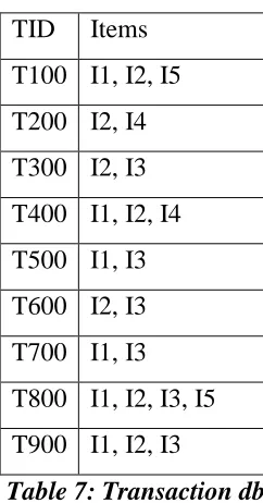
Input: Transaction db (Table 7), min-support count=2, Candidate items= {I1, I2, I3, I4, I5} Output: frequent itemset list.
Step 1: frequent 1 itemsets in descending order of support count
28
TID Items T100 I1, I2, I5 T200 I2, I4 T300 I2, I3 T400 I1, I2, I4 T500 I1, I3 T600 I2, I3 T700 I1, I3 T800 I1, I2, I3, I5 T900 I1, I2, I3
Table 7: Transaction db
The set of frequent items is sorted in the order of descending support count. This resulting set is denoted by L. Thus, we have L = {{I2: 7}, {I1: 6}, {I3: 6}, {I4: 2}, {I5: 2}}. Each transaction in the input transaction table, Table 7, is now sorted in the descending order of the support counts of the items in the transaction. Table 8 shows the sorted items in each transaction.
TID Items T100 I2, I1, I5 T200 I2, I4 T300 I2, I3 T400 I2, I1, I4 T500 I1, I3 T600 I2, I3 T700 I1, I3 T800 I2, I1, I3, I5 T900 I2, I1, I3
29
Step 2: Fp-tree construction
An FP-tree is then constructed as follows. First, create the root of the tree, labeled with “null.” Scan database (Table 8) once. The items in each transaction are processed in L order (i.e., sorted according to descending support count), and a branch is created for each transaction. For example, the scan of the first transaction, “T100: I1, I2, I5,” which contains three items (I2, I1, I5 in L (descending) order), leads to the construction of the first branch of the tree with three nodes, I2:1, I1:1, I5:1, where I2 is linked as a child to the root, I1 is linked to I2, and I5 is linked to I1. The second transaction, T200, contains the items I2 and I4 in L order, which would result in a branch where I2 is linked to the root and I4 is linked to I2. However, this branch would share a common prefix, I2, with the existing path for T100. Therefore, we instead increment the count of the I2 node by 1, and create a new node, I4: 1, which is linked as a child to I2: 2. In general, when considering the branch to be added for a transaction, the count of each node along a common prefix is incremented by 1, and nodes for the items following the prefix are created and linked accordingly.
Figure 9: Construction of fp tree
30
Step 3: Mining the fp-tree for frequent itemsets
Mining of the FP-tree is summarized in Table 9 and detailed as follows. We first consider I5, which is the last item in L. I5 occurs in two FP-tree branches of Figure 9. (The occurrences of I5 can easily be found by following its chain of node-links). The paths formed by these branches are I2, I1, I5: 1 and I2, I1, I3, I5: 1. Therefore, considering I5 as a suffix, its corresponding two prefix paths are I2, I1: 1 and I2, I1, I3: 1, which form its conditional pattern base. Using this conditional pattern base as a transaction database, we build an I5-conditional FP-tree, which contains only a single path, (I2: 2, I1: 2); I3 is not included because its support count of 1 is less than the minimum support count. The single path generates all the combinations of frequent patterns: {I2, I5: 2}, {I1, I5: 2}, {I2, I1, I5: 2}. Similar to the preceding analysis, I3’s conditional pattern base is {{I2, I1: 2}, {I2: 2}, {I1: 2}}. Its conditional FP-tree has two branches, I2: 4, I1: 2 and I1: 2, which generates the set of patterns {{I2, I3: 4}, {I1, I3: 4}, {I2, I1, I3: 2}} .This process is carried out for all the items.
Item Conditional pattern base Conditional FP-Tree Frequential Pattern Generated I5 [(I2 I2 :1),(I2 I1 I3:1)] (I2 :2,I1:2) I2I5:2, I1I5:2, I2I1I5:2
I4 [(I2 I1 :1),(I2 :1)] (I2 :2) I2I4:2
I3 [(I2 I1 :I2),(I2 :2),(I1:2)] (I2 :4,I1:2)(I2 :2) I2I3:4, I1I3:2, I1I3:2
I1 [(I2 :4)] (I2 :4) I2I1:4
Table 9: Final result
The final frequent itemset list is the union of all the frequent itemsets found so far. In our example, the final frequent itemset list F= I1, I2, I3, I4, I5, (I2, I5), (I1, I5), (I2, I1, I5), (I2, I4), (I2, I1), (I2, I3), (I1, I3), (I2, I1, I3).
31
candidate generation. It is a scalable technique for frequent pattern mining. Some disadvantages of FP tree is that tree is expensive to build.
2.2 Frequent Sequence mining algorithms
2.2.1 GSP Algorithm
The candidate generation method that is used in this algorithm will be used in the proposed algorithm. Generalized Sequential Patterns (GSP), an Apriori-based sequential pattern mining algorithm was introduced by Srikant and Agrawal (1996). The GSP algorithm makes multiple passes over the data. The first pass determines the frequent 1-item patterns (L1). Each subsequent pass starts with a seed set: the frequent sequences found in previous pass (Lk-1). The seed set is used to generate new candidate sequences (Ck). The candidate sequences are found using the GSP gen join. The GSP candidate generation method consists of 2 steps: Join phase and Prune phase. In order to obtain the k-sequence candidates (Ck), the frequent sequences found in previous step (Lk-1), joins with itself in an Apriori-gen way. This requires that every sequence - s in 1 joins with other sequences - s’in Lk-1, if the last elements of s (excluding the first element of s) is same as first elements of s’ (excluding the last element of s’). For example, sequence s-<(1) (2) (3)> can join with sequence s’- <(2) (35)>, since the last elements of s (ie. (2) (3)) is same as first elements of s’ (ie. (2)(3)). After the join phase, in the prune phase, the candidate sequences (Ck) that do not satisfy the minimum support count are removed to get the next frequent sequences (Lk+1). This process is repeated till no more candidate sequence sets can be generated. The final frequent sequence list is union of all frequent sequences found so far. In order to understand the candidate generation method used in the algorithm, we shall run through an example from the input to the final output of the algorithm.
Input: Sequence table (Table 10), minimum support count=2, Candidate items= {A, B, C, D, E, F, G}
32
Step 1: Finding frequent 1 items
From the given sequence table (Table 10), we get a frequent 1 table (Table 11) by eliminating all items that have support count less than the given min support count 2.
SID Sequences
1 <AB(FG)CD>
2 <BGD>
3 <BFG(AB)>
4 <F(AB)CD>
5 <A(BC)GF(DE)>
Table 10: GSP sequence table
Items Count
A 4
B 5
C 3
D 4
F 4
G 4
Table 11: Frequent-1 items
Step 2: Generating candidate sets and finding frequent sequences
33
an Apriori-gen way. This requires that every sequence - s in Lk-1 joins with other sequences - s’in Lk-1, if the last elements of s (excluding the first element of s) is same as first elements of s’ (excluding the last element of s’). For example, sequence s-<(1) (2) (3)> can join with sequence s’- <(2) (35)>, since the last elements of s (ie. (2) (3)) is same as first elements of s’ (ie. (2)(3)). After the join phase, in the prune phase, the candidate sequences (Ck) that do not satisfy the minimum support count are removed to get the next frequent sequences (Lk+1). For example, in Table 12, sequence (1,2) (3) joins with (2) (3,4) since the last 2 items (2,3) in the first sequence and the first 2 items (2,3) in the second sequence are the same. Equally, (1,2) (3) joins with (2) (3) (5). The join operation then produces (1,2) (3,4) and (1,2) (3) (5). In this example, Sequence (1,2) (3) (5) is pruned since its contiguous sub-sequence (1,2) (5) is not frequent (not in frequent 3-sequence).
Table 12: Candidate sequences generated using GSP-gen join
34
Figure 10: Final frequent sequences
The candidate generation method used in this algorithm will be used in the proposed TidFSeq algorithm for mining multiple sequence tables.
2.2.2 SPAM algorithm
35
the process of generating itemset-extended sequences is known as the item-extension step (abbreviated, the I-step). Let us consider an example to understand the algorithm.
Input: transaction db (Table 13), min-support count=2, Candidate items= {a, b, c, d} Output: frequent sequences
Step 1: Converting database to vertical bitmap
Sort the Database (Table 13) of itemsets in ascending Order of Cid and Tid. Store it in the form of vertical bitmap by setting (1) or (0) for itemsets depending on whether the item is found for a given transaction belonging to a specific sequence (Figure 11). For example, item 'a' is found in transaction ids: 1, 4, 5, the bits corresponding to those positions are set to 1 and other bits are set to 0.
CID TID Itemset
1 1 {a,b,d}
1 3 {b,c,d}
1 6 {b,c,d}
2 2 {b}
2 4 {a,b,c}
3 5 {a,b}
3 7 {b,c,d}
36
Figure 11: Vertical Bitmap of items in transaction db
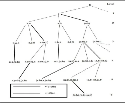
Step 2: Constructing lexicographic tree
37
Figure 12: Lexicographic tree
Step 3: Finding frequent sequences
38
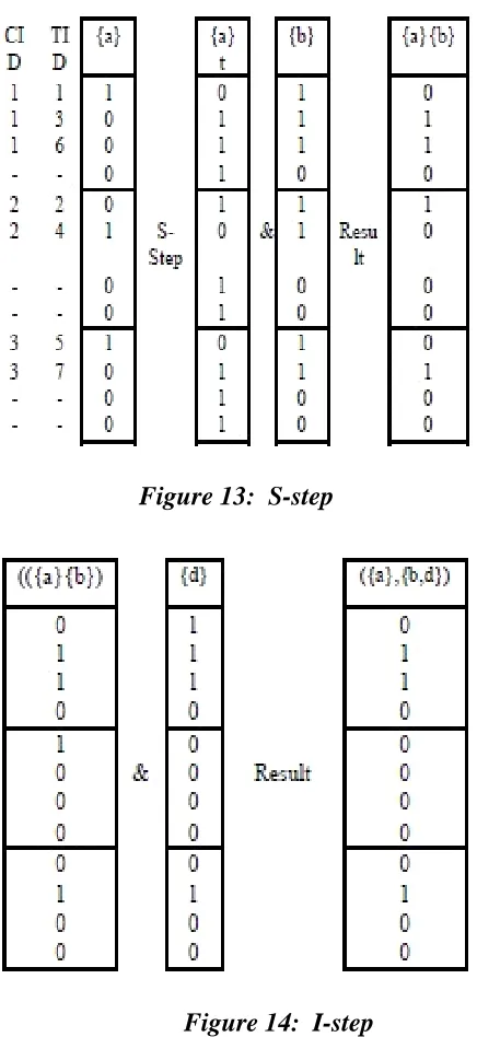
Figure 13: S-step
Figure 14: I-step
39
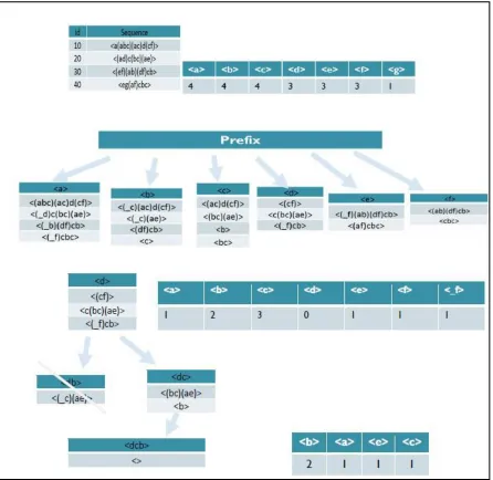
For I-step, we simply do the bit-AND operation on the bitmaps say for e.g. of ({a}, {b}) and {d} to get the result of ({a},{b,d}). Considering the first customer (sequence id) in the final bitmap, the second bit and the third bit for the first customer have value one. This means that the last itemset (i.e. {b}) of the sequence appears in both transaction 2 and transaction 3, and itemset {a} appears in transaction 1. After I-step or S-step is finished, we accumulate the number of sequences that have more than one ‟true‟ bits in bitmap results. As shown in Figures 13 and 14, it can be seen that the support count of ({a}, {b}) is 4 and that of ({a},{b,d}) is 3. If min sup is set to 50% (i.e., 2 sequences), both ({a}, {b}) and ({a},{b,d}) will be viewed as frequent and will not be pruned, else will be pruned. Following this procedure, SPAM can generate the complete set of frequent sequential patterns by traversing only through parent sequences which are frequent in the lexicographic tree, since by the Apriori principle, any child sequence generated from a infrequent parent sequence will not be frequent.
Key features and shortcomings: SPAM (Ayres and et al (2002)) outperformed SPADE (Zaki (2001)) and PrefixSpan (Pei and et al.(2004)) in terms of short runtime for relatively large datasets (20 transactions) size, because of vertical bitmap representation used for counting recursively many times. For the same reasons as the average number of items per transaction and the average number of transactions per customer increases, and as the average length of maximal sequences decreases, the performance of SPAM increases even further relative to the performance of SPADE and PrefixSpan. Scans the original database once and transforms it into vertical bitmap table unlike Apriori based approaches which requires multiple database scans. Storage Space: Because SPAM uses a depth-first traversal of the search space, it is quite space-inefficient in comparison to SPADE/PrefixSpan. SPAM uses the vertical bitmap representation to store transactional data, for each item we need one bit for transaction in the database.
2.2.3 PrefixSpan algorithm