Scholarship at UWindsor
Scholarship at UWindsor
Electronic Theses and Dissertations Theses, Dissertations, and Major Papers
4-13-2017
Prediction of High-Throughput Protein-Protein Interactions for
Prediction of High-Throughput Protein-Protein Interactions for
Large Datasets Using Repeated Random Sampling with
Large Datasets Using Repeated Random Sampling with
Replacement of Short Linear Motifs
Replacement of Short Linear Motifs
Behzad Rezaei
University of Windsor
Follow this and additional works at: https://scholar.uwindsor.ca/etd
Recommended Citation Recommended Citation
Rezaei, Behzad, "Prediction of High-Throughput Protein-Protein Interactions for Large Datasets Using Repeated Random Sampling with Replacement of Short Linear Motifs" (2017). Electronic Theses and Dissertations. 5950.
https://scholar.uwindsor.ca/etd/5950
Interactions for Large Datasets Using Repeated
Random Sampling with Replacement of Short
Linear Motifs
By
Behzad Rezaei
A Thesis
Submitted to the Faculty of Graduate Studies through the School of Computer Science in Partial Fulfillment of the Requirements for
the Degree of Master of Science at the University of Windsor
Windsor, Ontario, Canada
2017
c
Repeated Random Sampling with Replacement of Short Linear Motifs
by
Behzad Rezaei
APPROVED BY:
S. Nkurunziza
Department of Mathematics and Statistics
R. Gras
School of Computer Science
A. Ngom, Advisor School of Computer Science
L. Rueda, co-Advisor School of Computer Science
I hereby certify that I am the sole author of this thesis and that no part of this thesis has been published or submitted for publication.
I certify that, to the best of my knowledge, my thesis does not infringe upon anyones copyright nor violate any proprietary rights and that any ideas, techniques, quotations, or any other material from the work of other people included in my thesis, published or oth-erwise, are fully acknowledged in accordance with the standard referencing practices. Fur-thermore, to the extent that I have included copyrighted material that surpasses the bounds of fair dealing within the meaning of the Canada Copyright Act, I certify that I have ob-tained a written permission from the copyright owner(s) to include such material(s) in my thesis and have included copies of such copyright clearances to my appendix.
Wet-lab experimental methods for prediction of Protein-Protein Interactions (PPIs), as a decisive problem in biology, are labor demanding and costly, and usually comprise high false-negative and false-positive rates [20]. Therefore, computational methods have been extensively used as faster, less-expensive and more accurate alternatives [1]. Among all dif-ferent computational approaches for predicting PPIs, methods based on protein sequences information are more common than the others [16]. While such methods do not need any extra knowledge or data about the proteins rather than their sequences’ amino acids infor-mation, they have shown to be promising about predicting PPIs [16].
Basically, these methods try to find patterns spread over interacting and non-interacting proteins’ sequences, take them as features, and use them for predicting PPIs. Motifs, as common patterns of amino acids between a group of sequences [33], have been recently used for this purpose. There are some algorithms and tools for obtaining motifs from protein sequences. However, most of them have limitations on size of the datasets they can deal with, and also depend on datasets of pre-found motifs. One of the most popular algorithms which is capable of handling big datasets is Multiple EM for Motif Elucidation (MEME). Nevertheless, even for powerful tools like MEME, finding large number of motifs from such datasets would be time-wise infeasible.
I would like to express my deepest appreciation to my supervisor Dr. Alioune Ngom, and my co-supervisor Dr. Luis Rueda for their perpetual supports, patience, and inspiration during my Master’s program in University of Windsor. It was such an honor for me to know you, and also be in your research team. Thank you so much for giving me an opportunity to learn from you.
Secondly, I would also like to express my gratitude to my committee members Dr. Severien Nkurunziza, and Dr. Robin Gras for their beneficial advices and suggestions to my thesis.
Meanwhile I would like to express my special thanks to my friends for helping me during past two years.
DECLARATION OF ORIGINALITY III
ABSTRACT IV
AKNOWLEDGEMENTS V
DEDICATION VI
LIST OF TABLES IX
LIST OF FIGURES XI
1 Introduction 1
1.1 Protein-Protein Interaction . . . 1
1.2 Motifs . . . 2
1.2.1 Short Linear Motifs . . . 2
1.2.2 Tools for Finding Motifs . . . 3
1.3 Machine Learning . . . 6
1.4 WEKA as a classification and feature selection tool . . . 7
1.4.1 Classification algorithms . . . 7
1.4.2 Feature selection . . . 9
1.4.3 Evaluation method . . . 10
1.5 Motivation of this Thesis . . . 11
2 Literature review 13 2.1 Approaches for Prediction of PPIs . . . 13
2.1.1 Prediction of High-throughput Protein-Protein Interactions and Calmodulin-Binding Using Short-Linear Motifs . . . 13
2.1.2 A model based on minimotifs for classification of stable protein-protein complexes . . . 20
2.2 Inspiration from the Previous Works . . . 23
3 Materials and Methods 24 3.1 Datasets . . . 24
3.2 Obtaining protein sequences . . . 26
3.3 Refining the datasets . . . 28
3.4 Obtaining the SLiMs . . . 30
3.5 Finding and scoring the sites . . . 35
3.6 Building final datasets . . . 37
4.1.1 NaiveBayes . . . 42
4.1.2 KNN . . . 43
4.1.3 Random Forest . . . 44
4.1.4 SVM . . . 44
4.2 Classification results on datasets after feature selection . . . 47
4.2.1 Results of applying NaiveBayes on filtered datasets . . . 48
4.2.2 Results of applying KNN on filtered datasets . . . 48
4.2.3 Results of applying Random Forest on filtered datasets . . . 49
4.2.4 Results of applying SVM on filtered datasets . . . 49
4.3 Comparison . . . 52
4.3.1 Comparison of classifiers performances on original datasets . . . . 52
4.3.2 Comparison of classifiers performances on filtered datasets . . . 53
4.3.3 Original datasets VS filtered datsets . . . 54
4.3.4 Motifs VS Nomad . . . 56
5 Conclusion and Future Work 57 5.1 Contributions . . . 57
5.2 Future Work . . . 58
References 59
1.2.1 Comparing different motif discovery tools based on their platforms, type of the motif can be discovered by them, and their limitations. . . 6
4.1.1 Results of running Naive Bayes classifier on series 1 to 4, Stiff-Motifs, Flexible-Motifs, and Nomad-Motifs datasets. (Best,second best, andthird best). . . 43 4.1.2 Results of running KNN classifier (k=1 to k=70) on series 1 to 4,
Stiff-Motifs, Flexible-Stiff-Motifs, and Nomad-Motifs datasets. (Best, second best, andthird best). . . 44 4.1.3 Results of running Random Forest classifier on series 1 to 4, Stiff-Motifs,
Flexible-Motifs, and Nomad-Motifs datasets. (Best,second best, andthird best). . . 45 4.1.4 Grid-search on SVM reveals the best obtained results for each of seven
datasets. Values are gained accuracy(%) after running SVM on datasets. . . 46 4.1.5 Results of running SVM-RBF classifier on series 1 to 4, Stiff-Motifs,
Flexible-Motifs, and Nomad-Motifs datasets. (Best,second best, andthird best). . . 47 4.2.1 Number of features selected by mRmR for each dataset. . . 47 4.2.2 Results of running Naive Bayes classifier on series 1 to 4, Stiff-Motifs,
Flexible-Motifs, and Nomad-Motifs datasets after getting filtered using fea-ture selection results. (Best,second best, andthird best). . . 48 4.2.3 Results of running KNN classifier on series 1 to 4, Stiff-Motifs,
Flexible-Motifs, and Nomad-Motifs datasets after getting filtered using feature se-lection results. (Best,second best, andthird best). . . 49 4.2.4 Results of running Random Forest classifier on series 1 to 4, Stiff-Motifs,
filtered using feature selection results . Values are gained accuracy(%) after running SVM on datasets. . . 51 4.2.6 Results of running SVM-RBF classifier on series 1 to 4, Stiff-Motifs,
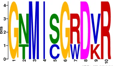
1.2.1 A Short Linear Motif (SLiM) of length 10, shown with logo and its corre-sponding regular expression. . . 2 1.4.1 Symbolic view of KNN for K=1, and K=3. . . 8 1.4.210-fold cross validation scheme. . . 10
2.1.1 Classification results for the score matrices with SLiMs obtained from the CM approach. . . 16 2.1.2 Classification results for the score matrices with SLiMs obtained from the
SM approach. . . 16 2.1.3 Prediction of PPIs using SVM-Polynomial (C = 1, 10, 100, 1000, gamma
= 0.01, 0.1, 0, 1, 10, 100, 1000) with SLiMs obtained from SM. . . 17 2.1.4 Prediction of PPIs using SVM-Polynomial (C = 1, 10, 100, 1000, gamma
= 0.01, 0.1, 0, 1, 10, 100, 1000) with SLiMs obtained from CM. . . 17 2.1.5 Prediction of CaM-binding proteins classification results for the score
ma-trices with SLiMs obtained from SM. . . 18 2.1.6 Prediction of CaM-binding proteins classification results for the score
ma-trices with SLiMs obtained from CM. . . 18 2.1.7 Prediction of CaM-binding proteins using SVMPolynomial (C = 1, 10, 100,
1000, gamma = 0.01, 0.1, 0, 1, 10, 100, 1000) with SLiMs obtained from SM. . . 19 2.1.8 prediction of CaM-binding proteins using SVMPolynomial (C = 1, 10, 100,
1000, gamma = 0.01, 0.1, 0, 1, 10, 100, 1000) with SLiMs obtained from CM. . . 19 2.1.9 KNN classification results for the datasets using PPI-SLIM-SEQ. . . 22 2.1.10SVM and LDR classification results for the ZH and MW datasets with the
been used for each part. . . 25
3.1.1 Samples from PrePPI dataset. Each row indicates there is an interaction between specified pair of proteins. . . 26
3.1.2 Samples from Negatome v 2.0 dataset. Each row indicates there is no in-teraction between specified pair of proteins. . . 26
3.2.1Sequencetag in P22619.xml file (downloaded from Uniprot.org) contains the sequence information for P22619 protein. . . 27
3.2.2 Our datasets view after finding the sequences information and changing their formats to FASTA. . . 27
3.3.1 Samples of duplicate protein pairs in Negatome dataset. . . 28
3.3.2 Algorithm used for finding duplicate protein pairs in our datasets. . . 28
3.3.3 Examples of identical protein pairs found using BLASTp results. . . 29
3.3.4 Corresponding sequences of discovered identical pairs. . . 29
3.3.5 Algorithm used for randomly selecting the positive and negative samples. . 30
3.4.1 Samples of discovered motif locations after using ANR mode in MEME. . . 32
3.4.2 Dividing the whole dataset into 100 subsets of size 50 pairs of protein (25 positive and 25 negative) in order to pass each subset to MEME separately and obtain 50 motifs of length 3 to 10. . . 32
3.4.3 Creating four different series of 100 subsets by shuffling the dataset, ran-domly selecting protein pairs, and putting them into subsets for each series. 33 3.4.4 Position Specific Probability Matrix (PSPM) for one discovered motif, and the regular expression obtained by that. . . 34
3.5.1 Samples of listed discovered motifs from series 1. . . 35
3.5.2 Algorithm used for scoring the sites. . . 36
entitled ”Flexible-Motifs” . . . 40
4.3.1 Comparing performance of each classifier over all original datasets. . . 53 4.3.2 Comparing performance of each classifier over all filtered datasets. . . 54 4.3.3 Comparing results of classifying each dataset, before and after feature
se-lection. . . 55 4.3.4 Time spent to discover 5000 motifs with MEME and Nomad. . . 56 4.3.5 Comparing the best result obtained from motifs discovered by MEME, with
Introduction
1.1
Protein-Protein Interaction
Binding two or more proteins with each other is called protein-protein interaction (PPIs) [26]. There are many indispensable biological processes happening in every living cell, which are affected by PPIs. Thus, to comprehend fundamental systems engaged in cellu-lar precesses studying these biological interactions is very important [28]. In other words, since for many proteins the only way to play their role in a cell is to interact with other companion proteins, Protein-Protein Interactions (PPIs) are, as a result, critical in discern-ing most of the biological processes existdiscern-ing in the cell [1]. PPIs analysis can assist both anticipating the function of the proteins that have not been discovered yet, and also distin-guishing fundamental pathways and processes at the cellular level [1]. Besides, information obtained from protein-protein interactions also helps to describe the function of a protein by its position in the protein-protein interaction network. Having this information will likely make a contribution to finding new drug targets [41].
Basically, common understanding of PPIs is mainly extracted from experimental meth-ods or computational indicator techniques [1]. Experimental methmeth-ods are costly, labor-intensive, and usually suffering from high false-positive and false-negative rates. Therefore, establishing trustworthy computational methods for predicting PPIs is of great importance [25].
information, and integration of sequence information and 3D structural information, re-spectively [23]. However, the first method is more common due to the fact that it does not depend on further information about proteins [16].
1.2
Motifs
Patterns outspread over a set of proteins which are functionally linked or may share bio-logical characteristics are called motifs [33]. In other words, motifs are frequent subse-quences occurring the most among a group of protein sesubse-quences [33]. Motifs can perform in an organized manner to show the complicatedness of practical regulatory inside the cell. Therefore, motif analysis will increase the knowledge about main process that runs protein-protein interactions [18].
1.2.1
Short Linear Motifs
While a motif consists of a sequence pattern of 3-20 amino acids, Short linear motifs (SLiMs) or minimotifs are referred to motifs with length of 3-10 amino acids[11], often with a mixture of fixed positions and wildcards[13].
SLiMs have been found to be decisive due to their capability of domain binding, con-version, cleavage, and targeting, which are all critical in signalling in cells [18]. A motif can be shown in two different ways, with its logo and its regular expression.
1.2.2
Tools for Finding Motifs
In last decades more research have been done on protein sequences and motifs, because of the important role that PPIs and SLiMs play in the function and formation of a protein. Having different ideas and algorithms finally led to have many databases and tools for ex-tracting motifs from the protein sequences. Most of these databases and tools are presented to the researchers and users only in a web-based platform, whereas some of them have pro-vided a standalone version of their tools as well. The advantage of using web-based tools, specially for small tasks, is that there is no need to go through any installation process, all users have to do is to enter the sequences they want to extract SLiMs from, customize their search parameters, submit the request to the server, and get the results on the browser. However all the web-based tools have limitation on the size of the input dataset.
Some of the main and popular tools for motif discovery are as follows:
• SLiMSearch
• SLiMFinder
• SLiMScape
• Eukaryotic Linear Motif (ELM)
• Minimotif Miner (MnM)
• Nomad
• MEME suite
user-decided SLiMs, then all the sites are scored using pre-schemed databases. Acording to the authors, SLiMSearch is developed to help clarifying the outputs of another SLiM discovery tool designed by the same authors called SLiMFinder.
According to Edwards et al. [13] SLiMFinder is a web-based and also standalone tool suitable for exploring high-throughput motifs. As they explain, SLiMFinder consists of two algorithms named SLiMBuild and SLiMChance. The authors claim that SLiMBuild first finds all the fixed length motifs, and keeps only those have been repeated between the sequences for adequate number of times. Then, it merges the selected motifs to obtain final ones containing wildcards. As they state, SLiMChance algorithm then evaluates probability of gained motifs, fixes their length and arrangements, and finally scores all the motifs.
Both SLiMSearch and SLiMFinder are valuable tools for motif discovery. however, as the authors claim [10] they both are designed for small protein datasets (up to 100 proteins for SLiMFinder [13]).
According to O’Brien et al. [43] SLiMScape is an add-on for Cytoscape which allows users to both search for sites of known motifs and also detecting new motifs. As the authors explain, SLiMScape has two main search tool. First, SLiMFinder which discovers new motifs by investigation a network of protein interactions, and second, SLimSearch which is able to detect sites of known or promising motifs through the same network. As they state, in last step results are illustrated by Cytoscape imagery features. The authors also state that internet connection is necessary while using SLiMScape, since it relies upon some websites like SMART domain database, Uniprot protein database, DBFetch, SLiMFinder, and SLiMSearch.
According to Dinkel et al. [12] Eukaryotic Linear Motif (ELM) has two main parts. First, a database of known motifs, and second, a web-based tool that uses this database to find potential motifs in provided protein sequence dataset. As Gould et al. [15] explain, users can provide protein sequences via ELM main page and will obtain the results of applicant motifs. The authors state that for educational goals, ELM also produces typed analysis and links to the literatures related to the roles that LM plays in the cell.
Minimo-tif Miner 3.0, the latest version released, has around 300,000 minimoMinimo-tifs from any species. As they explain while MnM 1.0 as the first version of this web service, did not have any filter on false positive cases and used to score the minimotifs based on the complicatedness of the sequences, MnM 2.0 let users to filter the results as needed. As the authors claim, basically filtering will not cut out the false positives, and it just assists the end user to filter the output based on his/her judgement. As the authors state, MnM 3.0 has significantly enhanced over MnM 2.0 in terms of accuracy of the minimotif searching, and also the size of the known minimotifs database.
According to Hernandez et al. [19] Nomad (Neighborhood Optimization for Multiple Alignment Discovery) is a local tool and also web interface that uses hill-climbing strategy and Ungapped Local Multiple Alignment (ULMA) to find non-overlapping fixed-size sites. As they explain, Nomad uses frequency of symbols of each position in ULMA to score obtained occurrences. The authors also claim that Nomad outperforms MEME and Gibbs Site Sampler in cases that sequences are distantly-related.
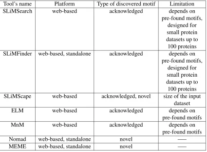
Tool’s name Platform Type of discovered motif Limitation
SLiMSearch web-based acknowledged depends on
pre-found motifs, designed for small protein datasets up to 100 proteins SLiMFinder web-based, standalone acknowledged depends on
pre-found motifs, designed for small protein datasets up to 100 proteins SLiMScape web-based acknowledged, novel size of the input
dataset
ELM web-based acknowledged depends on
pre-found motifs
MnM web-based acknowledged depends on
pre-found motifs
Nomad web-based, standalone novel —–
MEME web-based, standalone novel —–
TABLE 1.2.1: Comparing different motif discovery tools based on their platforms, type of the motif can be discovered by them, and their limitations.
For our experiment we need a motif discovery tool which has two characteristics. First, since our dataset is large and also the number of motifs to be found is large, query can not be processed via web-based platforms. Thus, the tool has to have standalone (local) version with no limitation on the size of either dataset or the number of requested motifs. Second, for prediction of PPIs we need to discover novel motifs. Therefore, the tool should be capable of finding novel motifs. Taking these facts and Table 1.2.1 into consideration, we decided to use MEME and Nomad for our experiments.
1.3
Machine Learning
as precise as possible [36]. In Machine learning, whenever the class labels of the data are known in advance (supervised learning), classification methods are used for prediction, otherwise (unsupervised learning) clustering techniques are needed [35].
1.4
WEKA as a classification and feature selection tool
Waikato Environment for Knowledge Analysis (WEKA) is one of the best and well-known tools that is widely used for machine learning and data mining [17]. With providing com-plete selection of machine learning algorithms, and data preparing gadgets, it helps users to easily classify new datasets with different machine learning algorithms and compare the results [17]. Besides, having an open source code has given users the ability of making and developing new projects which helps WEKA to enhance even more [17]. In classification, first a model is learned by training instances, then the learned model is used to classify the new examples into the acknowledged classes [39]. Classification process is as follows :
1. Building a training dataset
2. Analyzing the class feature and classes
3. Analyzing effective attributes for classification
4. Learning the model by the training samples in training set
5. Using the model to analyze the undiscovered data samples [39]
1.4.1
Classification algorithms
Bayesian classifiers, which rely on Bayes’ theory, are statistical classifiers [22]. To facilitate the associated computation, Naive Bayesian classifiers consider that impact of a class or feature value is autonomous and separated from other features [22]. Despite of this feeble independence hypothesis, the results of this classifier have shown to be promising and even in some cases comparable with more complicated methods [31]. Naive Bayes has been found to be efficient in many sensible functions such as medical analysis, and text labelling [31].
K-nearest neighbour (KNN) is one of the aged and elementary classification algorithms, and is one of the best options specially when there is no previous information about the data distribution [29]. KNN uses distance metrics (usually Euclidean distances) to find K-nearest neighbours of unknown samples in the data distribution space, to finally decide which class it belongs to based on the classes of its neighbours [46].
? ? 1 1 1 1 1 3 1 1 1 1 1 2 2 2 2 2 4 2 2 2 2 2
FIGURE 1.4.1: Symbolic view of KNN for K=1, and K=3.
Random Forest (RF) is an ensemble tree-based classifier that applies Bootstrap aggre-gating (bagging) method to make training sets [7]. It consists of two main techniques. First, random feature subspace which helps to build the trees faster, and second out-of-bag error which increases the chance of assessing the context of the features [7]. Generally, Random Forest is not parametric, has good accuracy, and able to discover importance of the features [32].
non-linearly separable data. Considering that Support Vectors (SV) are referred to the data points that lie on the very edge of each class, for linearly separable cases SVM tries to find a hyperplane that separates classes with the maximum margin [21]. Margin is any positive distance between the hyperplane and any data points. Once the optimum hyperplane is found, the resolution is defined by a linear mixture of involved support vectors [21].
However, the most realistic problems are non-linearly separable. For these cases SVM uses kernels to map the data onto higher dimensional space and then tries to find separating hyperplane in the new space [21]. Thus, a linear solution in the new feature space cor-responds to non-linear function in the initial space [21]. There are different kernels (like Polynomial, Radial Basis Function (RBF), Spline) with various options implemented for SVM. Therefore, in order to find the one that works the best for a given dataset, testing kernels with different combination of their options is suggested.
1.4.2
Feature selection
Since many of the classification methods are not initially devised to deal with multiple unrelated features, it is essential to mix them with feature selection (FS) methods [35]. Feature selection, which can be applied on both supervised and unsupervised learning, has three main goals:
1. to prevent over-fitting and promote model and prediction efficiency
2. to produce more agile and cost-efficient models
3. to obtain better understanding of how data is created [35]
1.4.3
Evaluation method
The method that is usually used for evaluating classifiers is called M-fold cross validation. In M-fold cross validation, which is a generalization of cross validation, first dataset is divided intomdisarranged sets of balanced size. Then the classifier is trainedmtimes such that at each iterationm-1folds are used to train the dataset and 1 fold is left out for testing. Finally, measures obtained from all M-folds are averaged (Figure 1.4.2).
FIGURE 1.4.2: 10-fold cross validation scheme.
Measures usually used for evaluating performance of a classifier are Accuracy, Sensi-tivity(Recall),Specificity, Precision, andMatthews Correlation Coefficient(MCC) which all are computed based on Confusion Matrix. Considering we have two classes, positive and negative, confusion matrix consists of four elements, TP, TN, FP, and FN [45]:
• True Positives (TP) are positive samples classified as positive
• True Negatives (TN) are negative samples classified as negative
• False Positives (FP) are negative samples classified as positive
• False Negatives (FN) are positive samples classified as negative
Accuracy = T P +T N
T P +F P +T N+F N (1.4.1)
Sensitivity(Recall) = T P
T P +F N (1.4.2)
Specif icity = T N
F P +T N (1.4.3)
P recision= T P
T P +F P (1.4.4)
M CC = √ T P ×T N −F P ×F N
(T P +F P)(T P +F N)(T N +F P)(T N+F N) (1.4.5)
Sensitivity (Recall) shows true positive rate, Specificity reveals true negative rate, Pre-cision offers positive predicted value [45], and MCC, which is a value between -1 and +1, presents the correlation coefficient among the classes and predicted samples. Where -1 means no correlation between predicted classes and actual classes, 0 means the perfor-mance of the classifier is not better than randomly classifying the samples, and +1 means precise prediction.
1.5
Motivation of this Thesis
Basically, these methods try to find patterns spread over interacting and non-interacting proteins’ sequences, take them as features, and use them for predicting PPIs. Motifs, as common patterns of amino acids between a group of sequences [33] , have recently been used for this purpose.
Many different tools have been developed for motif discovery. However, most of them usually have two major drawbacks for predicting PPIs using novel motifs. First, they have been designed to match possible motifs with a dataset of known motifs instead of uncov-ering new motifs, which leads to using motifs that are less appropriate for PPI prediction. Second, they have limitations on the size of the input dataset as well as on number of re-quested motifs, which leads to not having enough features for PPI prediction. Furthermore, even for a few tools that do not have these disadvantages (such as MEME), finding only hundreds of motifs may take months or years. Considering the fact that researchers in this area always tend to enlarge the dataset they are working on to obtain as close results as possible to the actual PPI datasets, existing boundaries have always inhibited them from achieving their goal.
In this thesis, we propose a method for obtaining large number of motifs from a large dataset of interacting and non-interacting proteins using MEME in much faster time. We obtained 5000 motifs from a database of size 5000 (pairs of proteins) and used discovered motifs to predict PPIs using classification methods. Our method proves to be encouraging specially considering the time spent to uncover 5000 novel motifs, and indicates that SLiMs are highly suitable for accurate prediction of PPIs.
Literature review
Among all the studies that have been done regarding using protein sequence information for predicting protein-protein interactions (PPI), using SLiMs has been the most popular. In this chapter we review some of the literature about short linear motifs for prediction of PPIs.
2.1
Approaches for Prediction of PPIs
2.1.1
Prediction of High-throughput Protein-Protein Interactions and
Calmodulin-Binding Using Short-Linear Motifs
According to Y. Li [24], prediction of protein-protein interactions (PPIs) and also Calmod-ulin Binding Proteins (CaM-binding) are two vital problems in biology. Existing methods for PPIs prediction are not usually precise enough and suffer from significant rates of FP and FN, besides developed methods for CaM-binding prediction are not advanced enough. The author states that in proposed method novel SLiMs found by MEME are used to predict PPIs and CaM-binding.
Previous work and shortcomings by others referred to by the authors
The new idea that the authors proposed
As Y. Li [24] claims, she has applied two different methods for obtaining SLiMs using MEME tool, SM and CM. She explains that SM means obtaining SLiMs from interacting and non-interacting datasets individually, while CM means putting both datasets together for SLiMs discovery. As the author describes, first she has applied SM and CM on both PPIs and CaM-binding datasets to discover 100 novel SLiMs for each set, then she scores the occurrences (sites) with 5 different functions, and finally uses gained scores to build the final datasets for prediction.
Materials and methods
As the author claims [24], for PPIs dataset 50 protein pairs has been downloaded from PrePPI dataset and set as positive samples, and 38 negative protein pairs has been obtained from Negatome Database version 2.0. On the other hand, for CaM-binding dataset 194 positive samples have been chosen from Calmodulin Target Database and 193 negative instances have been selected from Uniprot database. As the author explains, in proposed method MEME tool is used for discovering 100 motifs of length 3 to 10 for each dataset and each method (SM, and CM). Then 5 different methods have been used for scoring the occurrences (sites) as follows:
1. Counting sites
2. Scoring sites with I formula
I(a|X) = −
l
X
i=1
P(ai)×log(P(ai)) (2.1.1)
3. Scoring sites with ˆI formula
ˆ
I(a|X) =−1
l × l
X
i=1
P(ai)×log(P(ai)) (2.1.2)
5. SlidingWindow Scoring method
As the author clarifies, first method simply tries to find obtained motifs in original protein sequences and count the number of occurrences, while in second and third methods mentioned formulas has been used for calculating the scores of sites. As the author states [24], ”in the formulasXis the profile sequence,P(ai)is the probability (of theithresidue
ofa)”, andlis the length of the motif. According to the author, while the fourth method is actually the third scoring formula divided by the first one with the aim of checking the effects of counting sites on the ˆI formula, the fifth method considers every sub-sequence of lengthlin a sequence to likely be a site. Thus, a Sliding Window has been used to score all the possible sites.
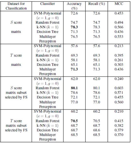
According to the author, in next step final datasets has been built based on the obtained scores, and different classification methods such as SVM-Polynomial kernel, Random For-est, KNN, and Multilayer Perceptron have been applied on the original dataset as well as dataset filtered by feature selection method.
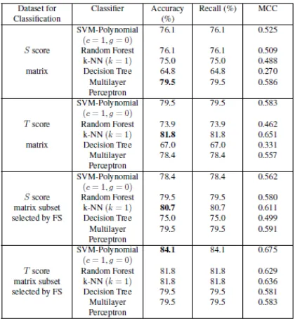
Results that the authors claim to have achieved
FIGURE 2.1.1: Classification results for the score matrices with SLiMs obtained from the CM approach.
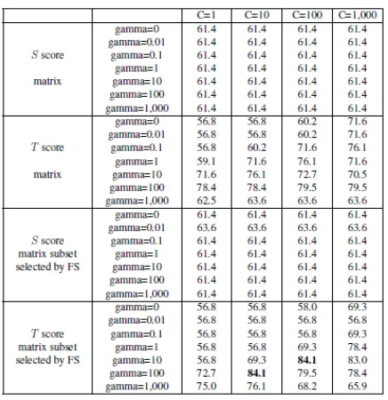
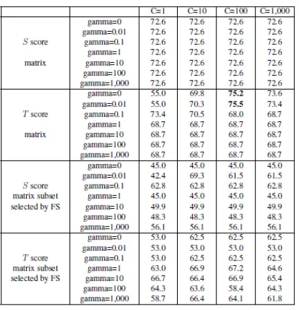
FIGURE 2.1.3: Prediction of PPIs using SVM-Polynomial (C = 1, 10, 100, 1000, gamma = 0.01, 0.1, 0, 1, 10, 100, 1000) with SLiMs obtained from SM.
FIGURE 2.1.4: Prediction of PPIs using SVM-Polynomial (C = 1, 10, 100, 1000, gamma = 0.01, 0.1, 0, 1, 10, 100, 1000) with SLiMs obtained from CM.
The Author also claims to have obtained the following results for CaM-Binding predic-tion using her methods on the datasets menpredic-tioned above:
FIGURE 2.1.5: Prediction of CaM-binding proteins classification results for the score ma-trices with SLiMs obtained from SM.
FIGURE 2.1.7: Prediction of CaM-binding proteins using SVMPolynomial (C = 1, 10, 100, 1000, gamma = 0.01, 0.1, 0, 1, 10, 100, 1000) with SLiMs obtained from SM.
FIGURE 2.1.8: prediction of CaM-binding proteins using SVMPolynomial (C = 1, 10, 100, 1000, gamma = 0.01, 0.1, 0, 1, 10, 100, 1000) with SLiMs obtained from CM.
they got better accuracy compared to result obtained from original dataset.
2.1.2
A model based on minimotifs for classification of stable
protein-protein complexes
According to L.Rueda et al. [34] prediction of obligate and non-obligate proteins is an important problem in biology. As they explain, between all different existing problems in this matter, they aimed their attention at the problem of distinguishing the immobility of protein structure, and the transportation from non-obligate to obligate. As the authors clarify, obligate interactions are easier to investigate due to the fact that they are continuous, while non-obligate interactions are acknowledged to be either long-lasting or short-term.
Previous work and shortcomings by others referred to by the authors
The authors [34] refer to the related work that addresses the related problem of prediction of protein-protein interaction types using association rule based classification [27], and pre-diction of biological protein-protein interactions using atom-type and amino acid properties [2], and also predicting and analyzing protein-protein interaction types using electrostatic energies [44], and state that the shortcomings of previous work are first, methods using protein structures are restricted to structural information of the proteins which with cur-rent knowledge is accessible for a small number of proteins, and second such methods are basically slow and time-absorbing.
The new idea that the authors proposed
Materials and methods
As the authors [34] claim, they have used two different datasets named ZH and MW. As they explain, ZH includes 75 obligate and 62 non-obligate curated pairs of proteins obtained from [49], while MW contains 115 obligate and 212 non-obligate curated pairs of protein. They also explain that they have used MEME to obtain two series of 1000 SLiMs, first of length 3-10 , and second of length 2-7 for each ZH and MW, separately.
According to the authors [34], after discovering the motifs each sequence is divided into all attainable overlapping small frames of lengthl(equal to SLiMs length), then using un-covered SLiMs information content for each frame is determined by the following formula, and finally best 20 values are used to build 20 feature vector for each pair of protein.
ˆ
I(a|X) =−1
l × l
X
i=1
P(ai)×log(P(ai)) (2.1.3)
As the authors add, since log(1) = 0, in order to avoid losing information the following cases have been applied while scoring the frames:
logP(ai) =
log(0.99) ifP(ai) = 1
log(P(ai)) otherwise
(2.1.4)
its capacity of generalization and independence of acknowledged features.
Results that the authors claim to have achieved
The Author claims to have obtained the following results using their methods on the datasets mentioned above:
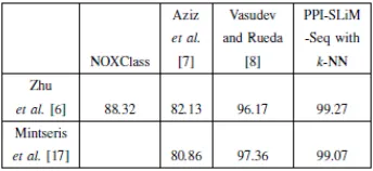
FIGURE 2.1.9: KNN classification results for the datasets using PPI-SLIM-SEQ.
FIGURE 2.1.10: SVM and LDR classification results for the ZH and MW datasets with the MW and ZH SLiMs respectively.
FIGURE 2.1.11: Comparison of classification accuracy with other related works.
is 99.27% forl=9,7,6,5 for ZH dataset and the same accuracy for l=8,5 for MW dataset. They also claim that best obtained results for SVM is 98.77% accuracy which is obtained from MW dataset, using ZH SLiMs and withl=6, while for LDR classifier the best gained result is for quadratic kernel with 99.27% accuracy from the ZH dataset, using MW SLiMs.
2.2
Inspiration from the Previous Works
Materials and Methods
In this chapter we describe the dataset and methods we used in our experiments step by step. As illustrated in Figure 3.0.1, Java is used for most of the parts that required text-file processing and scoring. We used Python to extract the sequences from the corresponding proteins XML files downloaded from UniProt website [www.Uniprot.org] (a hub for pro-tein information) [9]. BLASTp software and also Java used for purifying the dataset, and MEME is used for obtaining the SLiMs. We benefited from java.regex for finding the sites, and used WEKA for classification and feature selection purposes.
3.1
Datasets
FIGURE 3.1.1: Samples from PrePPI dataset. Each row indicates there is an interaction between specified pair of proteins.
FIGURE 3.1.2: Samples from Negatome v 2.0 dataset. Each row indicates there is no interaction between specified pair of proteins.
Since we wanted to deal with balanced datasets, we selected the same number of protein pairs from each datasets (PrePPI and Negatome). Ideally, we should have selected as much pairs as existing in the smaller dataset which is 4397 (from Negatome). However, in order to make our datasets more manageable we reduce the size of each dataset to 3500. Using Java Random class, we randomly selected 3500 positive protein pairs from PrePPI dataset as well as 3500 negative protein pairs from Negatome dataset.
3.2
Obtaining protein sequences
FIGURE 3.2.1: Sequencetag in P22619.xml file (downloaded from Uniprot.org) contains the sequence information for P22619 protein.
After obtaining protein sequences we changed our datasets format from the original one (Figure 3.1.1, and 3.1.2) to FASTA format (Figure 3.2.2). In FASTA format first line of each entry, which is indicated by a>symbol, is a description line for that entry, and is followed by sequence information of corresponding protein in next line(s). The reason we changed our datasets to FASTA format is that FASTA is one of the layouts that is acceptable by most of the motif discovery tools as well as blast software.
3.3
Refining the datasets
In this part we curated our datasets by finding repeated and duplicate pairs in our datasets in order to have clean datasets with unique instances.
1. Duplicate protein pairs
As we noticed both PrePPI and Negatome databases happens to have duplicate pro-tein pairs such that two or more different rows indicate interact or non-interact inter-action between same pair of proteins. In order to refine the datasets, using Java codes (Figure 3.3.2) we found these repeated samples, kept one for each pair and removed duplicates from our datasets. In this code, we compared each pair of proteins with rest of the pairs to see if we could find cases such that proteins in a pair are repeated with any order in another pair.
FIGURE 3.3.1: Samples of duplicate protein pairs in Negatome dataset.
2. Different proteins with identical sequences
There are some proteins in both PrePPI and Negatome database such that they have different names, they have identical sequences though. Since our method depends on protein sequences, having such instances can affect the SLiMs discovery part and eventually our classification results. In order to avoid these proteins, we applied a BLASTp query on our datasets, found such samples, saved one for each pair and eliminated remaining duplicates.
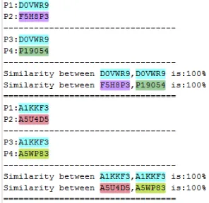
FIGURE 3.3.3: Examples of identical protein pairs found using BLASTp results.
FIGURE 3.3.4: Corresponding sequences of discovered identical pairs.
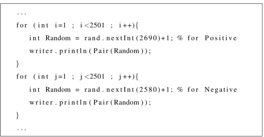
we randomly chose 2500 protein pairs from remaining pairs in each class (Figure 3.3.5). RAND function in Java produces a random number between 0 and the number provided for rand.nextInt() - 1.
FIGURE 3.3.5: Algorithm used for randomly selecting the positive and negative samples.
3.4
Obtaining the SLiMs
As mentioned earlier, we used MEME for motif discovery part. However, regardless of all the benefits that MEME has such as having standalone version which removes limitations on input dataset size and also capability of discovering novel motifs, finding even hundreds of motifs would be infeasible due to the long time that it takes. Considering for our case we have to look for motifs of length 3 to 10, the time needed to obtain motifs gets even longer than usual since all the process has to be repeated over and over again for each value of the length of the motif.
Undoubtedly, the obtained motifs from a set of proteins depends on existing proteins in that set. In order to check how different grouping (making subsets randomly) may change the motifs and eventually the classification results we decided to obtain four different series of 100 subsets with completely unlike arrangement. Thus, after dividing the dataset into 100 subsets we shuffled the whole dataset and repeated grouping part to create second, third, and fourth random series of 100 subsets (Figure 3.4.2). While finding 5000 motifs from a dataset of size 5000 (protein pairs) may take several months or years, we obtained 20,000 motifs (5000 motifs from each series) only in 40 days.
For each series we passed each subset to MEME separately to obtain 50 motifs of length 3 to 10 using the following command:
meme Dataset.txt -o SubsetName -mod anr -nmotifs 50 -minw 3 -maxw 10
where Dataset.txt is the dataset created for each subset (25 positive and 25 negative pairs), -o indicates the name of the output folder, -mod signifies the mode for obtaining the motifs, -nmotifs specifies the number of motifs that need to be discovered, and -minw and -maxw are the minimum and maximum length of motifs, respectively.
MEME has three different modes for discovering motifs:
1. Zero or one occurrence per sequence (ZOOPS)
2. One occurrence per sequence (OOPS)
3. Any number of repetitions (ANR)
FIGURE 3.4.1: Samples of discovered motif locations after using ANR mode in MEME.
FIGURE 3.4.3: Creating four different series of 100 subsets by shuffling the dataset, ran-domly selecting protein pairs, and putting them into subsets for each series.
MEME will create a logo for each one of the discovered motifs, as well as one output text file for each executed and terminated command (in our case for each subset). This text file contains information about sequences existing in the input dataset, letter frequency in the dataset, as well as Position Specific Probability Matrix (PSPM) for each discovered motif. For all discovered motifs we used PSPM to uncover their regular expression.
sponding residue, otherwise the probability is distributed between more than one residue, which means that position in the pattern has a wild-card of all corresponding residues. Fi-nally, the regular expression is obtained by attaching all fixed and wild cards from the first position to the last one.
3.5
Finding and scoring the sites
After obtaining regular expression of all discovered motifs, we used Java regular expres-sion (java.util.regex package) to find and score the sites. Java Regex is a package that helps to find a substring in another string. All it needs is a pattern written in regular expression form, and a string that is going to be searched. The former is calledPattern, and the latter is named Matcher. For example, running following pattern and matcher in java will give us the number of matches found (here is 2) as well as starting position of the matches:
Pattern r = Pattern.compile(”M[LRC]V”);
Matcher m = r.matcher(”PDTMLVCSVLVLLLRRNMRVNGDS”); While (m.find( ))
Thus, in order to build our final dataset based on the discovered motifs, for each pair of protein we passed all 5000 discovered motifs to the pattern separately to count all matches in both protein sequences.
FIGURE 3.5.1: Samples of listed discovered motifs from series 1.
sequence to the ”Matcher” and try to do the same. Eventually, we do the same for all 5000 motifs (Figure 3.5.2).
FIGURE 3.5.2: Algorithm used for scoring the sites.
Using regular expression pattern and matcher, this code will find all the sites existing in both proteins sequences and count number of matches for each motif (Figure 3.5.3).
3.6
Building final datasets
Using mentioned method (Figure 3.5.2), we built our final dataset such that for each pair of proteins in our dataset we assigned score of each motif in its corresponding position.
FIGURE 3.6.1: Building the final dataset based on the scores provided by the regular expression.
Since we had four different series of 5000 motifs, we created one dataset, as explained, for each series to see how different grouping changes the classification results. Further-more, at this point we decided to score all 20,000 motifs and created two more datasets based on the flexibility of motifs patterns.
It has been proved that motifs can be scored using information theory [14]. Thus we use following formula to score each motif (all logarithms are base 2):
I(P) =X
i
H(M)−H(Ki) (3.6.1)
H(P) =−X
a∈C
PalogPa (3.6.2)
where C is a set of symbols {a}, which each of them has a background probability
I(P)by the length of the motifs to normalize the scores. Therefore, we have:
I(P) =
P
iH(M)−H(Ki)
l (3.6.3)
wherelis the length of each motif.
For example, for pattern K = C[DG][AHQ]D, while M ={A,C,D,P,G,H,Q}, and their background probabilities arePA=PC =PD =PG =PH =PQ = 16, and considering that
probabilities of letters in a wild-card are equal, scoring would be as follows:
I(P) =
P
iH(M)−H(Ki)
l =
H(M)−H(C)+H(M)−H([DG])+H(M)−H([AHQ])+H(M)−H(D)
l =
−6(16log16)+1log1−6(16log16)+2(12log12)−6(16log16)+3(13log13)−6(16log16)+1log1
4 =
7.7548
4 = 1.9387
As mentioned earlier, using (3.6.3) we scored all 20,000 motifs obtained from the four series. Then, we used the 5000 top scored ones to create a new dataset named (Stiff-Motifs), and also used 5000 low scored ones to create another dataset named (Flexible-Motifs). The reason for choosing these names is that the motifs with higher scores have more fixed-card and do not have flexible positions (Figure 3.6.2), while motifs with lower scores have more wild-cards and as a result they are more flexible (Figure 3.6.3). It means the lower score a motif has, there is more chance to find sites using that motif, because it has more wild-cards.
3.7
Classification
Results
For classification purposes, we used different classifiers such as Naive Bayes, K-nearest neighbour (KNN), Random Forest, and SVM with two different kernels, Polynomial and Radial Basis Function (RBF) on all of our datasets. As mentioned earlier, we had six datasets created by the SLiMs obtained using MEME(four datasets from four series of subsets and two datasets using scoring function, named Stiff-Motifs and Flexible-Motifs), and one dataset which was built using SLiMs discovered by Nomad.
After obtaining the results, we also applied Feature Selection on all datasets with the aim of removing possible noise and obtaining better results. For mRmR we selected ” Wrap-perSubsetEval” as ”Attribute evaluator” and ”RerankingSearch” as its search method. Fur-thermore, we chose Random Forest as wrapper’s classifier, andAccuracyfor its evaluation measure. Moreover, we used mRmR as our ranking method.
We used the features selected by mRmR to filter our datasets, and applied all mentioned classifiers once again on filtered datasets to be able to compare both methods. The results of classifying all datasets (original and filtered) using the mentioned classifiers, as well as comparison between the two methods are listed and discussed in this chapter.
4.1
Classification results on the original datasets
4.1.1
NaiveBayes
0.528 MCC. Besides, NaiveBayes could not classify Stiff-Motifs with better than 61.14% accuracy.
Naive Bayes Confusion Matrix Accuracy(%) Precision(%) Recall(%) MCC
Series 1 1208 1292 72.46 79.30 72.50 0.513
85 2415
Series 2 1277 1223 73.38 79.20 73.40 0.522
108 2392
Series 3 1248 1252 73.28 79.80 73.30 0.527
84 2416
Series 4 1176 1324 71.60 78.50 71.60 0.496
96 2404
Stiff-Motifs 2478 22 61.14 76.30 61.10 0.343
1921 579
Flexible-Motifs 1271 1229 73.52 79.60 73.50 0.528
95 2405
Nomad-Motifs 2496 4 71.88 81.80 71.90 0.528
1402 1098
TABLE 4.1.1: Results of running Naive Bayes classifier on series 1 to 4, Stiff-Motifs, Flexible-Motifs, and Nomad-Motifs datasets. (Best,second best, andthird best).
4.1.2
KNN
KNN Confusion Matrix Accuracy(%) Precision(%) Recall(%) MCC
Series 1 (k=2) 2226 274 90.52 90.60 90.50 0.811
200 2300
Series 2 (k=3) 2201 299 90.96 91.10 91.00 0.821
153 2347
Series 3 (k=1) 2178 322 90.78 91.00 90.80 0.818
139 2361
Series 4 (k=2) 2242 258 90.62 90.60 90.60 0.813
211 2289
Stiff-Motifs (k=1) 2464 36 72.24 80.80 72.20 0.523
1352 1148
Flexible-Motifs (k=2) 2210 290 90.68 90.80 90.70 0.814
176 2324
Nomad-Motifs (k=1) 1517 983 78.98 83.50 79.00 0.623
68 2432
TABLE 4.1.2: Results of running KNN classifier (k=1 to k=70) on series 1 to 4, Stiff-Motifs, Flexible-Stiff-Motifs, and Nomad-Motifs datasets. (Best,second best, andthird best).
4.1.3
Random Forest
As shown in Table 4.1.3, applying Random Forest classifiers on 5 datasets Series 1, Series 2, Series 3, Series 4, and Flexible-Motifs gave us almost the same accuracy of 92%. While the best result is 92.36% accuracy and 0.847 MCC for Series 3, Random Forest could not classify Flexible-Motifs and Nomad-Motifs better than 72.52% and 79.30% accuracy, respectively.
4.1.4
SVM
Random Forest Confusion Matrix Accuracy(%) Precision(%) Recall(%) MCC
Series 1 2292 208 92.04 92.00 92.00 0.841
190 2310
Series 2 2298 202 92.08 92.10 92.10 0.842
194 2306
Series 3 2317 183 92.36 92.40 92.40 0.847
199 2301
Series 4 2282 218 91.50 91.50 91.50 0.830
207 2293
Stiff-Motifs 2462 38 72.52 80.80 72.50 0.527
1336 1164
Flexible-Motifs 2281 219 91.76 91.80 91.80 0.835
193 2307
Nomad-Motifs 1524 976 79.30 83.90 79.30 0.630
59 2441
TABLE 4.1.3: Results of running Random Forest classifier on series 1 to 4, Stiff-Motifs, Flexible-Motifs, and Nomad-Motifs datasets. (Best,second best, andthird best).
performance.
As shown, while the best accuracy for each dataset has been obtained with different mixture of cost and gamma, the best result for four out of seven datasets (Series 1, Series 3, Series 4, and Flexible-Motifs) has been obtained setting cost to 10 and gamma to 0.01. Considering that accuracy for all these 4 datasets are the best 4 accuracies among all 7 datasets we can realize that c=10 and g=0.01 is the best combination between all the ones we tried.
SVM Grid-Search Series 1 Series 2 Series 3 Series 4 Stiff-Motifs Flexible-Motifs Nomad-Motifs
SVM-Polynomial 51.00 52.40 51.30 51.10 50.10 56.30 50.02
SVM-RBFc=10,
g=0.01 92.24 92.22 92.32 91.24 72.60 93.70 78.18
SVM-RBFc=10,
g=0.1 91.60 91.76 92.06 90.68 72.62 87.60 74.32
SVM-RBFc=10,
g=1 82.82 82.18 78.78 82.00 71.02 63.40 76.42
SVM-RBFc=10,
g=10 71.96 70.74 66.58 68.98 69.90 52.80 81.00
SVM-RBFc=10,
g=100 71.96 70.74 66.58 68.98 69.90 52.80 81.00
SVM-RBFc=10,
g=1,000 71.96 70.74 66.58 68.98 69.90 52.80 81.00
SVM-RBFc=10,
g=5,000 71.96 70.74 66.58 68.98 69.90 52.80 81.00
SVM-RBFc=10,
g=10,000 71.96 70.74 66.58 68.98 69.90 52.80 81.00
SVM-RBFc=10,
g=20,000 71.96 70.74 66.58 68.98 69.90 52.80 81.00
SVM-RBFc=10,
g=100,000 71.96 70.74 66.58 68.98 69.90 52.80 81.00
SVM-RBFg=0.01,
c=1 89.96 89.14 89.72 88.18 68.20 92.40 72.98
SVM-RBFg=0.01,
c=10 92.24 92.22 92.32 91.24 72.60 93.70 78.18
SVM-RBFg=0.01,
c=100 91.80 92.64 92.26 91.12 72.92 93.40 79.38 SVM-RBFg=0.01,
c=1,000 91.48 90.10 91.74 90.36 72.86 92.80 79.20 SVM-RBFg=0.01,
c=10,000 90.52 90.10 90.32 88.46 72.90 92.50 79.20 SVM-RBFg=0.01,
c=100,000 89.40 89.46 89.94 87.84 72.90 92.50 79.20 SVM-RBFg=0.01,
c=1,000,000 89.02 88.78 89.94 87.94 72.90 92.50 79.20
SVM-RBF Confusion Matrix Accuracy(%) Precision(%) Recall(%) MCC
Series 1 (c=10, g=0.01) 2251 249 92.24 92.30 92.20 0.846
139 2361
Series 2 (c=100, g=0.01) 2276 224 92.64 92.70 92.60 0.853
144 2356
Series 3 (c=10, g=0.01) 2244 256 92.32 92.40 92.30 0.848
128 2372
Series 4 (c=10, g=0.01) 2209 291 91.24 91.40 91.20 0.826
147 2353
Stiff-Motifs (c=100, g=0.01) 2445 55 72.92 80.50 72.90 0.528
1299 1201
Flexible-Motifs (c=10, g=0.01) 2360 140 93.70 93.70 93.70 0.874
175 2325
Nomad-Motifs (c=10, g=10) 2074 426 81.00 81.00 81.00 0.620
524 1976
TABLE 4.1.5: Results of running SVM-RBF classifier on series 1 to 4, Stiff-Motifs, Flexible-Motifs, and Nomad-Motifs datasets. (Best,second best, andthird best).
4.2
Classification results on datasets after feature
selec-tion
As we mentioned, we used mRmR feature selection method with setting Random Forest as its wrapper’s classifier. The number of features that mRmR chose between all the features for each dataset (5000) is as follows:
Feature selection with mRmR Number of selected features
Series 1 25
Series 2 24
Series 3 27
Series 4 28
Stiff-Motifs 2
Flexible-Motifs 20
Nomad-Motifs 1
TABLE 4.2.1: Number of features selected by mRmR for each dataset.
see how feature selection affects the classification results.
4.2.1
Results of applying NaiveBayes on filtered datasets
As can be seen in Table 4.2.2, NaiveBayes classified Series 1, Series 2, Series 3, F-Series 4, and Flexible-Motifs datasets with accuracy between 69% to 74%. The best result is achieved from classifying F-Series 3 with 73.76% accuracy and 0.534 MCC. Besides, NaiveBayes could not classify F-Stiff-Motifs, and F-Nomad-Motifs datasets with better than 52.86%, and 51.98% accuracy.
Naive Bayes Confusion Matrix Accuracy(%) Precision(%) Recall(%) MCC
F-Series 1 1174 1326 71.92 79.20 71.90 0.506
78 2422
F-Series 2 1275 1225 73.76 80.00 73.80 0.534
87 2413
F-Series 3 1177 1323 72.06 79.40 72.10 0.509
74 2426
F-Series 4 1171 1329 71.72 78.90 71.70 0.501
85 2415
F-Stiff-Motifs 2498 2 52.86 75.10 52.90 0.169
2355 145
F-Flexible-Motifs 1043 1457 69.26 77.60 69.30 0.462
80 2420
F-Nomad-Motifs 2498 2 51.98 74.50 52.00 0.139
2399 101
TABLE 4.2.2: Results of running Naive Bayes classifier on series 1 to 4, Stiff-Motifs, Flexible-Motifs, and Nomad-Motifs datasets after getting filtered using feature selection results. (Best,second best, andthird best).
4.2.2
Results of applying KNN on filtered datasets
KNN (k=1 to k=70) Confusion Matrix Accuracy(%) Precision(%) Recall(%) MCC
F-Series 1 (k=2) 2041 459 85.96 86.20 86.00 0.722
243 2257
F-Series 2 (k=3) 2004 496 84.70 85.00 84.70 0.697
269 2231
F-Series 3 (k=1) 2067 433 86.54 86.80 86.50 0.733
240 2260
F-Series 4 (k=2) 2033 467 85.16 85.40 85.20 0.705
275 2225
F-Stiff-Motifs (k=1) 2497 3 54.08 75.40 54.10 0.203
2293 207
F-Flexible-Motifs (k=4) 2088 412 85.14 85.20 85.10 0.703
331 2169
F-Nomad-Motifs (k=1) 2498 2 51.98 74.50 52.00 0.139
2399 101
TABLE 4.2.3: Results of running KNN classifier on series 1 to 4, Stiff-Motifs, Flexible-Motifs, and Nomad-Motifs datasets after getting filtered using feature selection results. (Best,second best, andthird best).
4.2.3
Results of applying Random Forest on filtered datasets
As shown in Table 4.2.4, applying Random Forest classifiers on 5 datasets Series 1, F-Series 2, F-F-Series 3, F-F-Series 4, and F-Flexible-Motifs gave us accuracy between 85% and 88%. While the best result is 88.06% accuracy and 0.763 MCC for F-Series 3, Random Forest could not classify Stiff-Motifs and Nomad-Motifs better than 54.08% and 51.98% accuracy, respectively.
4.2.4
Results of applying SVM on filtered datasets
Random Forest Confusion Matrix Accuracy(%) Precision(%) Recall(%) MCC
F-Series 1 2033 467 86.00 86.30 86.00 0.723
233 2267
F-Series 2 2044 456 85.88 86.10 85.90 0.720
250 2250
F-Series 3 2128 372 88.06 88.20 88.10 0.763
225 2275
F-Series 4 2069 431 86.22 86.40 86.20 0.726
258 2242
F-Stiff-Motifs 2497 3 54.08 75.40 54.10 0.203
2293 207
F-Flexible-Motifs 2182 318 86.76 86.80 86.80 0.735
344 2156
F-Nomad-Motifs 2498 2 51.98 74.50 52.00 0.139
2399 101
TABLE 4.2.4: Results of running Random Forest classifier on series 1 to 4, Stiff-Motifs, Flexible-Motifs, and Nomad-Motifs datasets after getting filtered using feature selection results. (Best,second best, andthird best).
SVM Grid-Search F-Series 1 F-Series 2 F-Series 3 F-Series 4 F-Stiff-Motifs F-Flexible-Motifs F-Nomad-Motifs
SVM-Polynomial 70.24 75.10 74.40 74.90 54.08 80.34 51.98
SVM-RBFc=10,
g=0.01 84.18 83.88 85.86 84.50 54.08 84.88 51.98
SVM-RBFc=10,
g=0.1 85.52 85.42 87.30 86.20 54.08 87.92 51.98
SVM-RBFc=10,
g=1 86.08 85.76 87.78 86.08 54.08 85.58 51.98
SVM-RBFc=10,
g=10 85.80 84.92 87.34 84.72 54.08 79.52 51.98
SVM-RBFc=10,
g=100 85.80 84.92 87.34 84.72 54.08 79.52 51.98
SVM-RBFc=10,
g=1,000 85.80 84.92 87.34 84.72 54.08 79.52 51.98
SVM-RBFc=10,
g=5,000 85.80 84.92 87.34 84.72 54.08 79.52 51.98
SVM-RBFc=10,
g=10,000 85.80 84.92 87.34 84.72 54.08 79.52 51.98
SVM-RBFc=10,
g=20,000 85.80 84.92 87.34 84.72 54.08 79.52 51.98
SVM-RBFc=10,
g=100,000 85.80 84.92 87.34 84.72 54.08 79.52 51.98
SVM-RBFg=0.01,
c=1 82.94 83.06 84.66 82.94 53.76 83.06 51.98
SVM-RBFg=0.01,
c=10 84.18 83.88 85.86 84.50 54.08 84.88 51.98
SVM-RBFg=0.01,
c=100 84.34 84.42 85.98 84.66 54.08 85.18 51.98 SVM-RBFg=0.01,
c=1,000 84.02 84.48 86.14 84.94 54.08 85.40 51.98 SVM-RBFg=0.01,
c=10,000 84.38 83.82 85.76 84.58 54.08 84.70 51.98 SVM-RBFg=0.01,
c=100,000 84.92 83.68 86.06 83.88 54.08 83.94 51.98 SVM-RBFg=0.01,
c=1,000,000 82.70 76.66 84.36 82.16 54.08 78.44 51.98
SVM-RBF Confusion Matrix Accuracy(%) Precision(%) Recall(%) MCC
Series 1(c=10, g=1) 2067 433 86.08 86.20 86.10 0.723
263 2237
Series 2 (c=10, g=1) 2092 408 85.76 85.80 85.80 0.716
304 2196
Series 3 (c=10, g=1) 2164 336 87.78 87.80 87.80 0.756
275 2225
Series 4 (c=10, g=0.1) 2010 490 86.20 86.70 86.20 0.729
200 2300
Stiff-Motifs (c=10, g=0.1) 2497 3 54.08 75.40 54.10 0.203
2293 207
Flexible-Motifs (c=10, g=0.1) 2125 375 87.92 88.00 87.90 0.760
229 2271
Nomad-Motifs (c=10, g=0.1) 2498 2 51.98 74.50 52.00 0.139
2399 101
TABLE 4.2.6: Results of running SVM-RBF classifier on series 1 to 4, Stiff-Motifs, Flexible-Motifs, and Nomad-Motifs datasets after getting filtered using feature selection results. (Best,second best, andthird best).
4.3
Comparison
4.3.1
Comparison of classifiers performances on original datasets
scored motifs, which have more fixed-cards in their patterns than wild-cards, decreases the chance of finding sites, and consequently the quality of the dataset. Indeed, the best results for our last dataset, Nomad-Motifs, obtained from KNN, Random Forest, and SVM-RBF with almost 80% accuracy.
Finally, among all the classifiers we used in our experiment, SVM-Polynomial was the weakest and KNN, Random Forest, and SVM-RBF all performed very well. From another point of view, among all our datasets, Series 1, Series 2, Series 3, Series 4, Flexible-Motifs were almost equally the best datasets.
FIGURE 4.3.1: Comparing performance of each classifier over all original datasets.
4.3.2
Comparison of classifiers performances on filtered datasets
As shown in Figure 4.3.2, KNN, Random Forest, and SVM-RBF could classify F-Series 1, F-Series 2, F-Series 3, F-Series 4, and Flexible-Motifs filtered datasets all with around 85% accuracy, including the best result obtained from classifying F-Series 3 with Random Forest with 88.06% accuracy.
SVM-It can be concluded from the figure that KNN, Random Forest, and SVM-RBF all performed well classifying filtered datasets. Besides, among all filtered datasets F-Series 3, and Flexible-Motifs were the best ones.
FIGURE 4.3.2: Comparing performance of each classifier over all filtered datasets.
4.3.3
Original datasets VS filtered datsets
4.3.4
Motifs VS Nomad
As illustrated in Figure 4.3.4, Nomad is much faster than MEME in terms of discovering motifs, such that finding 5000 motifs with Nomad only takes less than 2 days, while it takes around 10 days to discover 5000 motifs with MEME.
FIGURE 4.3.4: Time spent to discover 5000 motifs with MEME and Nomad.
However, as shown in Figure 4.3.5, the best results that we could achieve among all the datasets created by motifs discovered by MEME was from classifying Flexible-Motifs dataset with SVM-RBF with almost 94% accuracy, while Nomad-Motifs dataset could never be classified with any classifier with more than 81% accuracy. Thus, in our case MEME proved to be a better tool for motif discovery.
Conclusion and Future Work
5.1
Contributions
We proposed a novel method to deal with the problem of finding large number of motifs from large datasets, and use them for prediction of protein-protein interactions. In our method, first we chose 2500 interacting and 2500 non-interacting protein pairs, and after curating the dataset, we divided the whole dataset into 100 small subsets and randomly selected 25 interacting and 25 non-interacting for each subset. Using the same idea we created three more series of subsets to see how different grouping changes the classification results. At this point, instead of passing the whole dataset to MEME, we separately passed subsets of each series to MEME to discover novel motifs. As explained earlier, we used a function to score all the motifs and created two more datasets based on the flexibility of the motifs. We also used Nomad to discover motifs from our original dataset to be able to compare the results of MEME and Nomad. After that we used five different classifiers to predict protein-protein interactions. We also used mRmR feature selection to see if it can help the classifiers with removing the noises.
accu-Flexible-Motif have always been either the best, or so close to the best. This proves that us-ing flexible motifs for creatus-ing the dataset enhances the performance of classifies, because having patterns with lower scores means having more wild-cards, which eventually leads to find more sites and have better dataset.
Although feature selection significantly enhanced the performance of SVM-Polynomial, the accuracy of other classifiers decreased by almost 5%. As a result, we state that in our case feature selection could not help classifiers to obtain better results in total.
5.2
Future Work
I divided the dataset into hundred subsets of size fifty protein pairs (half interacting and half non-interacting). Other combination of the number of subsets and their size can be taken into consideration for further studies. Besides, I simply added up the number of sites I found in each protein pairs to create final datasets. However, scoring the sites with existing formulas from other works may be used. Furthermore, the motifs selected by feature selection can somehow be related to each other. Studying their relation can be a possible extension to this work. Finally, other feature selection methods can be used with the aim of obtaining better results. Therefore, all options for extending this work can be summarized as follows:
• Changing the subsets number and size to see how enlarging or shrinking the subsets might change the classification results.
• Scoring the sites with different scoring functions.
• The relationship between the discovered motifs can be taken into consideration for further investigation.
[1] Ahmed, H. R. and Glasgow, J. I. J. (2014). Pattern discovery in protein networks reveals high-confidence predictions of novel interactions. AAAI, pages 2938–2945.
[2] Aziz, M., Maleki, M., Rueda, L., Raza, M., Banerjee, S., et al. (2011). Prediction of biological protein–protein interactions using atom-type and amino acid properties.
Proteomics, 11(19):3802–3810.
[3] Bailey, T. L., Bod´en, M., Whitington, T., and Machanick, P. (2010). The value of position-specific priors in motif discovery using meme. BMC Bioinformatics, 11(1):1.
[4] Bailey, T. L., Johnson, J., Grant, C. E., and Noble, W. S. (2015). The meme suite.
Nucleic Acids Research, 43(W1):W39–W49.
[5] Blohm, P., Frishman, G., Smialowski, P., Goebels, F., Wachinger, B., Ruepp, A., and Frishman, D. R. (2014). Negatome 2.0: a database of non-interacting proteins derived by literature mining, manual annotation, and protein structure analysis. Nucleic Acids Research, page gkt1079.
[6] Browne, F., Zheng, H., Wang, H., and Azuaje, F. (2010). From experimental ap-proaches to computational techniques: a review on the prediction of protein-protein interactions. Advances in Artificial Intelligence, 2010:7.
[8] Chang, C.-C. and Lin, C.-J. (2011). LIBSVM: a library for support vector machines.
ACM Transactions on Intelligent Systems and Technology (TIST), 2(3):27.
[9] Consortium, T. U. (2014). Uniprot: a hub for protein information. Nucleic Acids Research, page gku989.
[10] Davey, N. E., Haslam, N. J., Shields, D. C., and Edwards, R. J. (2011a). SLiM-Search 2.0: biological context for short linear motifs in proteins. Nucleic Acids Re-search, 39(suppl 2):W56–W60.
[11] Davey, N. E., Trav´e, G., and Gibson, T. J. (2011b). How viruses hijack cell regulation.
Trends in Biochemical Sciences, 36(3):159–169.
[12] Dinkel, H., Van Roey, K., Michael, S., Kumar, M., Uyar, B., Altenberg, B., Milchevskaya, V., Schneider, M., K¨uhn, H., Behrendt, A., et al. (2015). ELM 2016data update and new functionality of the eukaryotic linear motif resource. Nucleic Acids Research, page gkv1291.
[13] Edwards, R. J., Davey, N. E., and Shields, D. C. (2007). SLiMFinder: a probabilistic method for identifying over-represented, convergently evolved, short linear motifs in proteins. PloS one, 2(10):e967.
[14] Eidhammer, I., Jonassen, I. T., William, R., and Inge Jonassen, W. R. T. (2004).
Protein Bioinformatics: An algorithmic approach to sequence and structure analysis. John Wiley and Sons, Ltd.
[15] Gould, C. M., Diella, F., Via, A., Puntervoll, P., Gem¨und, C., Chabanis-Davidson, S., Michael, S., Sayadi, A., Bryne, J. C., Chica, C., et al. (2009). ELM: the status of the 2010 eukaryotic linear motif resource. Nucleic Acids Research, page gkp1016.