Adv. Radio Sci., 6, 139–143, 2008 www.adv-radio-sci.net/6/139/2008/
© Author(s) 2008. This work is distributed under the Creative Commons Attribution 3.0 License.
Advances in
Radio Science
Macro-modelling via radial basis functionen nets
C. Wiegand1,2, C. Fischer1, R. Kazemzadeh2,3, C. Hedayat1,2, W. John2, and U. Hilleringmann1 1University of Paderborn, Department of Electrical Engineering, Sensor Technology Group, Germany
2Fraunhofer Institute for Reliability and Microintegration (IZM) Advanced System Engineering (ASE), Paderborn, Germany 3Leibniz University of Hannover Institute of Electromagnetic Theory (TET), Hannover, Germany
Abstract. By the rising complexity and miniaturisation of the device’s dimensions, the density of the conductors creases considerably. Referring to this, locally transient in-teractions between single physical values become apparent. Therefore, for the investigation and optimisation of inte-grated circuits it is essential to develop suitable models and simulation surroundings which allow for memory and time-efficient calculation of the behaviour. By means of the dy-namic reconstruction theory and the radial basis functions nets the so-called black box models are provided. The de-scription of black box models is derived from the input and output behaviour or so-called time series of a dynamic sys-tem. Concerning the time series, the black box model adapts its parameters via the extended Kalman filter. This paper provides a modelling approach that enables fast and efficient simulations.
1 Introduction
The increasing simulation time is a big limiting factor dur-ing the design and the development of HDI/HDP systems. Hence, it is more and more crucial to provide models which allow for quick and accurate simulations (Wiegand et al., 2007b,a; Stievano, 2002). The classical modelling approach, based on the transistor level circuits and the symbolic anal-ysis, requires unreasonably long computation times. The black box modelling (BBM) via radial basis functions (RBF) nets for integrated circuits is an adequate solution that pro-vides robust and fast simulations. In the following, a method is presented for developing mathematical models to reduce the very growing simulation times for transient analysis. This modelling approach is based on the dynamic reconstruction of dynamic systems. That is, a mathematical formulation needs to be found, that describes the dynamics of the system to be examined as accurately as possible without necessarily considering the physical characteristics of the circuit.
Correspondence to: C. Wiegand
In Sect. 2 the modelling flow for developing black box mod-els is discussed, although the radial basis functions nets are the main focus of all considerations. Section 3 describes the architecture of the RBF nets. The parameter adaptation, i.e. the extended Kalman filter, is explained in Sect. 4. In Sect. 5 a NOR element with two inputs and three outputs is exam-ined. Then, an example of a diode is considered and the RBF model is parameterised in such a way so as to allow for the temperature to be regarded as a further input.
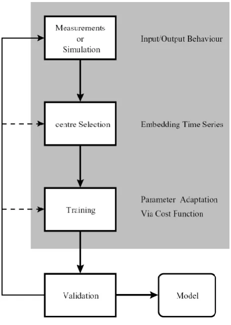
2 Modelling flow
Fig. 1. Modelling flow.
3 Radial basis functions nets
With using RBF networks, it is possible to represent any continuous nonlinear function. Because of this important feature, they are utilised to model nonlinear dynamic systems and integrated circuits. Radial basis functions nets are special feedforward neural networks consisting of three layers with a hidden layer.
Input layer: definition of the number of inputs, i.e. within the regressor vector the number of inputs is fixed.
Hidden layer: signal processing viapradial basis functions (Gaussian) or so-called neurons. Furthermore the embedding of the data occurs just in the hidden layer.
Output layer: definition of the number of outputs. Regarding
weighted transitions the neurons outgoing signals are added up within every output.
Figure 2 shows a schematic representation of a typical RBF network with multiple inputs and multiple outputs (MIMO). The response of a MIMO radial basis functions net
Fig. 2. Schematic representation of a multiple input and multiple output radial basis functions net.
can be formulated as follows:
ˆ
y1
.. .
ˆ
ym
=
θ11 · · ·θ1p ..
. . .. ...
θm1· · ·θmp
φ1(ζ1)
.. .
φp(ζp)
(1)
whereφi(ζi)denotes theit hgaussian activation function in the hidden layer and can be written as
φi(ζi)=e−ζi mitζ =(x−ci)T6−i1(x−ci) (2) andxis the regressor vector and is denoted by
x=hxT1,· · ·,xTniT. (3) Within the regressor vector the n inputs are de-fined; m and n describe the number of outputs and the number of basis functions; ci is the it h centre and 6i =diag(σi)=diag [σ12i,· · ·, σri2]represents the shape of theit hbasis function. Equation 1 can be described in the following way:
ˆ
y1
.. .
ˆ
ym
=
θT1
.. .
θTm
φ1(ζ1)
.. .
φp(ζp)
ˆ
y =2φ
. (4)
C. Wiegand et al.: Macro-modelling via radial basis functionen nets 141 time FIR1/IIR-Filters2 can be used instead of the weights
or global feedback paths (Howlett, 2001a,b) could be intro-duced. A simple method to create dynamics can be expressed by:
xi(t )=[ui(t−1),· · · , ui(t−d1),
yi(t−1),· · ·, yi(t−d2)]T , (5) whered1andd2denote the input embedding dimension and the output embedding dimension. By making such changes, a state space model can be described (Wiegand et al., 2007a). The first order derivation can be employed to transform the discrete time representation into a continuous state space model.
4 Parameter estimation
Generally, the parameters of a RBF net can be determined by a huge number by algorithms, for example, by the lo-cally regularised least square algorithm with centre selection (Chena et al., 1990a; Chen et al., 1990b, 1996). Nevertheless, non-linear optimisation methods must then be employed to adapt the shapes6i of the basis functions. Within this work, the extended Kalman filter (EKF) is used for parameter iden-tification of non-linear systems. In accordance to this, all parameters are determined iteratively by the EKF, including those which are in the argument of the gaussian function. For the initialisation and the improvement of the convergence, the K-Means cluster algorithms is used to determine the cen-tres. In addition, this cluster algorithm delivers an facile pos-sibility for the calculation of the shapes (widths) of the basis functions, to be able to determine the weights by means of least square methods.
4.1 K-Means cluster algorithm
The algorithm is an iterative procedure to divide a set of training data into groups (cluster). The only available in-formation is the training data and the number of the clus-ters. This is also known as unsupervised learning. A random choice of the cluster centresc(0)within the training setT
serves as the starting point. Next, in every iteration stepk, every set of trainig data is allocated to the nearest situated cluster centre and thus the subsets Mi are obtained. The identification of the new centres
ci(k+1)= 1
Ni X
x∈Mi
x (6)
is accomplished by means of average determination via the sets
Mi = {x∈T :ci(k)=argmin c(k)
kx−c(k)k2}, (7) 1FIR: Finite Impulse Response
2IIR: Infinite Impulse Response
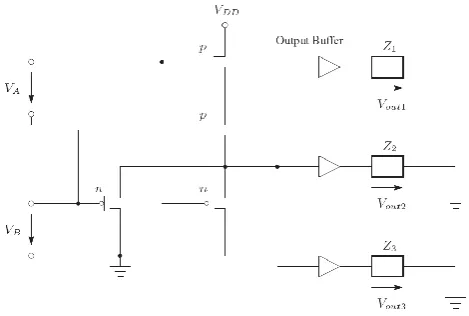
Fig. 3. NOR-Circuit with two inputs (VA undVB) and three out-puts (Vout1,Vout2undVout3). The buffers of the respective outputs are four cascaded inverters. Also, the outputs are concluded with different complex impedances (Zi, wherei∈[1,2,3]).
whereasNidenotes the number of elements which are in the setMi. An initialisation of the matrices6can take place af-ter the deaf-termination of the centres, i.e. afaf-ter the last iaf-teration step:
σi,j = v u u t
1
Ni X
x∈Mi
(xj −ci,j(K))2 (8)
σi = [σi,1,· · · , σi,r]T (9)
6i =(diag(σi))2 (10)
With the calculated initial centres and the widths of the ba-sis functions, it is possible to determine the weights, i.e., by utilising the least square methods.
4.2 Extended Kalman Filter
Iteratively, the EKF estimates the parameter vector
wk = h
θT1,· · · ,θTp,σT1,· · · ,σTp,cT1,· · ·,cTpiT. (11) using
wk =wk−1+Kke (12) whereKkis the Kalman gain.
Kk =Pk−1Hk h
Rk+HTkPk−1Hk i−1
(13)
e=y− ˆy is the error between the observed outputsy (target vector) and the estimated outputs yˆ of the RBF network;
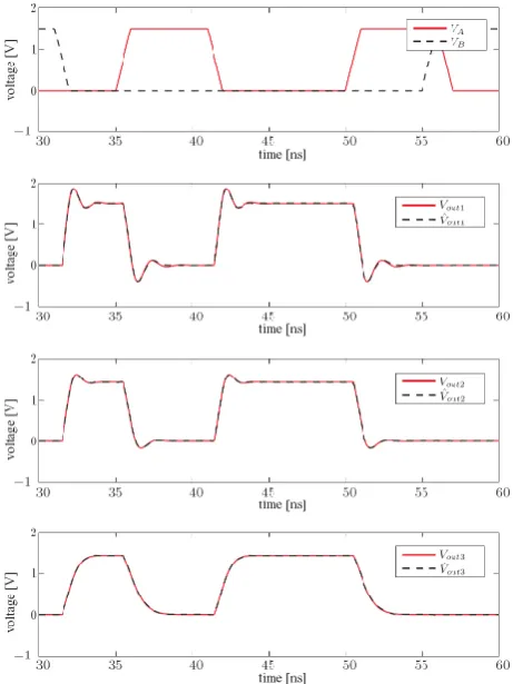
Fig. 4. Input and output signals of the simulated system and model. The output voltages marked with a hat denote the outputs of the RBF model.
∂fj(x,w) ∂ci
=2θj i6−i 1(x−ci) e−ζ (14)
∂fj(x,w) ∂θj i
=e−ζ (15)
∂fj(x,w) ∂σi
=2θj i6e
−1
i sq(x−ci)e−ζ (16)
wheree6iis defined as e
6i =diag(eσi)=diag
[σ13i,· · ·, σri3] (17) with
sq(x−ci)= [(x1−c1i)2,· · · , (xr −cri)2]T. (18) Rk andPk denote the variance of the measurement noise and the error covariance matrix. The error covariance matrix is a positive definite symmetricν×ν matrix, whereνis the number of parameters being updated and can be determined by:
Pk = h
I−KkHTk i
Pk−1+q0I. (19)
Fig. 5. Identity lines of the diode and the model for different tem-peratures.
According to Ahmida and Charef (2002), q0 regulates the allowed random step towards the gradient. For fast parameter estimation, the training data is subdivided into smaller sets. These sets are used to adjust the parameters of the RBF net. Afterwards, a test is performed as well as an update of the regressor vector.
5 Simulations
In the following section, two different nonlinear systems are considered.
The first example corresponds to a two input and three output NOR-Circuit (see Fig. 3). In the second example a diode is envisaged, in which the ability of parameterisation of the RBF nets is illustrated.
5.1 Example 1: NOR Circuit
C. Wiegand et al.: Macro-modelling via radial basis functionen nets 143
x(k)= h
uT(k),uT(k−1),yT(k−1)
iT
(20)
u(k)=[u1(k), u2(k)]T (21)
y(k)=[y1(k), y2(k), y3(k)]T (22) In Fig. 4 the input signals (VAundVB) as well as the re-sponse of the ADS-system (Vout1, Vout2 und Vout3) and the RBF model (Vˆout1,Vˆout2undVˆout3) are shown. The model is able to represent the dynamic as well as the logical behaviour of the system. The mean square error (MSE) is about 4·10−5. 5.2 Example 2: diode
The system under consideration is a diode (SISO), but the RBF net was implemented with a second input. This second input is virtual and corresponds to the parameterisation of the model taking the temperature drift into account. This means that the temperature is considered at the modelling level as if it were an other input. This is therefore a simple example that shows the ability to parameterise the RBF nets. The most simple identity equation is
y(k)=Is
eqUinkT −1, (23) whereUin denotes the input voltage, k andqstand for the Boltzmann constant and the elementary charge. Is is the saturation current and for simulation purposesIs was fixed to 5·10−3A. During the training, the temperature was var-ied between 18◦C to 33◦C. The training signal, consisting of
1000 values, had a sine-shaped course and formed, in combi-nation with the temperature, the two-dimensional regressor. For conclusive testing, four characteristic curves were sim-ulated for 21◦C, 24◦C, 27◦C und 30◦C (Fig. 5). The mean square error is in the order of magnitude 10−6.
6 Conclusions
In this paper it was explained how a MIMO RBF net can be generated by means of the K-Means cluster algorithm and the extended Kalman filter. It became apparent that it is pos-sible to model physical parameters in the same fashion. To achieve a noticeable gain in speed, the systems to be mod-elled must be substantially more complex. Nevertheless, it was shown that the RBF nets are able to carry out precise and fast system-level simulations. The future efforts will concen-trate on the application of the findings in a industrial envi-ronment.
Acknowledgements. The reported R+D work was carried out within
the MEDEAplus A701 PARACHUTE (Parasitic Extraction and Op-timization for Efficient Microelectronics System Design and Ap-plication) project. This particular research was supported by the BMBF (Bundesministerium fur Bildung und Forschung) of Federal Republic of Germany University of Paderborn under grant 01M 3169 E and Infineon Technologies AG under grant 01M 3169 A. The views expressed in this paper are those of the authors only.
References
Chen, S., Billings, S. A., Cowan, C. F. N., and Grant, P. M.: Non-linear system identification using radial basis functions, Int. J. Control, 21, 2513-2539, 1990a.
Chen, S., Billings, S. A., Cowan, C. F. N., and Grant, P. M.: Prac-tical identification of NARMAX models using radial basis func-tions, Int. J. Control, 52, 1327-1350, 1990b.
Chen, S., Chng, E. S., and Alkadhimi, K.: Regularized orthogo-nal least squares algorithm for constructing radial basis function networks, Int. J. Control, 64, 829-837, 1996.
Haykin, S.: Kalman Filtering and Neural Networks, John Wiley & Sons, Inc., New York, Chichester, Weinheim, Brisbane, Singa-pore, Toronto, 2001.
Howlett, R. J. and Jain, L. C.: Radial Basis Funcrion Networks 1 – Recent Developments in Theory and Application, Physica-Verlag, 2001a.
Howlett, R. J. and Jain, L. C.: Radial Basis Funcrion Networks 2 – New Advances in Design, Physica-Verlag, 2001b.
Sauer, T., Yorke, J. A., and Casdagli, M.: Embedology, J. Stat. Phys., 65, 579-616, 1991.
Sing, J. K., Basu, D. K., Nasipuri, M., and Kundu, M.: Improved K-means Algorithm in the Design of RBF Neural Networks, TEN-CON 2003, Conference on Convergent Technologies for Asia-Pacific Region, 2, 841-845, 2003.
Stievano, I. S., Maio, I. A., and Canavero, F. G.: Parametric Macro-models of Digital I/O Ports, IEEE T. Adv. Packaging, Special Selection on EPEP01, 25(2), 255–264, 2002.
Wiegand, C., Hedayat, C., John, W., Radic-Weissenfeld, L., and Hilleringmann, U.: Nonlinear Identification of Complex Systems using Radial Basis Function Networks and Model Order Reduc-tion, IEEE International Symposium on EMC, Honolulu Hawaii, USA, 2007a.
Wiegand, C., Radic-Weissenfeld, L., Hedayat, C., John, W.: Black Box Model and Singular Value Based Model Order Reduction, 18th International Zurich Symposium on EMC, 2007b.