Scholarship at UWindsor
Scholarship at UWindsor
Electronic Theses and Dissertations Theses, Dissertations, and Major Papers
2011
A New Cell-Centred Finite Difference Scheme for CFD Simulations
A New Cell-Centred Finite Difference Scheme for CFD Simulations
Ali Salih
University of Windsor
Follow this and additional works at: https://scholar.uwindsor.ca/etd
Recommended Citation Recommended Citation
Salih, Ali, "A New Cell-Centred Finite Difference Scheme for CFD Simulations" (2011). Electronic Theses and Dissertations. 5388.
https://scholar.uwindsor.ca/etd/5388
This online database contains the full-text of PhD dissertations and Masters’ theses of University of Windsor students from 1954 forward. These documents are made available for personal study and research purposes only, in accordance with the Canadian Copyright Act and the Creative Commons license—CC BY-NC-ND (Attribution, Non-Commercial, No Derivative Works). Under this license, works must always be attributed to the copyright holder (original author), cannot be used for any commercial purposes, and may not be altered. Any other use would require the permission of the copyright holder. Students may inquire about withdrawing their dissertation and/or thesis from this database. For additional inquiries, please contact the repository administrator via email
by
Ali Salih
A Thesis
Submitted to the Faculty of Graduate Studies
through Mechanical, Automotive and Materials Engineering in Partial Fulfillment of the Requirements for
the Degree of Master of Applied Science at the University of Windsor
Windsor, Ontario, Canada
2011
by
Ali Salih
APPROVED BY:
______________________________________________ Dr. Tirupati Bolisetti
Department of Civil and Environmental Engineering
______________________________________________ Dr. Biao (Bill) Zhou
Department of Mechanical, Automotive and Materials Engineering
______________________________________________ Dr. Ronald Barron, Advisor
Department of Mathematics and Statistics, and
Department of Mechanical, Automotive and Materials Engineering
______________________________________________ Dr. Bruce Minaker, Chair of Defense
Department of Mechanical, Automotive and Materials Engineering
AUTHOR’S DECLARATION OF ORIGINALITY
I, Ali Salih, hereby certify that I am the sole author of this thesis. This thesis includes original research that has been previously published/submitted for publication in peer reviewed conference proceedings, as follows,
Thesis Chapter Publication title/full citation Publication status
Chapter 3 & 4 Salih, A. and Barron, R.M. A New Cell-Centred
Finite Difference Scheme for CFD Simulations.
19th Annual Conf. of the CFD Society of Canada, Montreal, April 2011.
Presented
Chapter 3 & 4 Salih, A. and Barron, R.M. A Cell-Based Finite
Difference Method for the Numerical Solution of
PDEs. Applied Mathematics, Modeling and
Computational Science Conference, Waterloo, July 2011.
Accepted
I certify that the material contained in this thesis describes work completed during my registration as a graduate student at the University of Windsor.
I declare that, to the best of my knowledge, my thesis does not infringe upon anyone’s copyright nor violate any proprietary rights and that any ideas, techniques, quotations, or any other material from the work of other people included in my thesis, published or otherwise, are fully acknowledged in accordance with the standard referencing practices. Furthermore, I certify that I have not included copyrighted material that surpasses the bounds of fair dealing within the meaning of the Canada Copyright Act.
Provisional Patent Application 61/457,589 has been filed on April 22, 2011 for Patent Protection for: “Cell-Centered Finite Difference Method for Numerical Solution of Partial Differential Equations on Arbitrary Mesh Systems”
ABSTRACT
The governing partial differential equations of fluid motion are usually numerically approximated using one of the three classical methods: Finite Difference
(FD), Finite Volume (FV) or Finite Element (FE). In this thesis, a new cell-centred FD (CCFD) formulation is developed, in which the governing fluid flow equations are differenced over all the cell centres instead of grid points. The nodes (grid points) are
then updated by averaging the property from all the cell centres that share that node. This feature, which is motivated by development of the FV method, allows the application of
the proposed FD numerical formulation on unstructured grids. Several test cases are investigated here to illustrate this approach. To verify the results, the analytical solution for the test case is used if available. Otherwise, the numerical solution is compared to the
DEDICATION
ACKNOWLEDGEMENTS
I owe my deepest gratitude to my supervisor, Dr. Ronald Barron, whose guidance,
support and patience from the start to the final level of this project made this thesis possible.
TABLE OF CONTENTS
AUTHOR’S DECLARATION OF ORIGINALITY ... iii
ABSTRACT ... iv
DEDICATION... v
ACKNOWLEDGEMENTS... vi
LIST OF FIGURES ... x
LIST OF TABLES... xiii
NOMENCLATURE ... xiv
CHAPTER I. INTRODUCTION ... 1
II. REVIEW OF LITERATURE... 6
2.1 Introduction ... 6
2.2 Classical Numerical Schemes in CFD ... 6
2.3 Locating Variables and Related Issues in FV Method ... 8
2.4 Model Equation ... 10
2.5 Accelerating the Solution ... 11
2.6 Thesis Objectives ... 12
III. DESIGN AND METHODOLOGY ... 14
3.1 The CCFD Scheme ... 14
3.2 A Simple Test Problem ... 20
3.2.1 Solution procedure ... 20
3.2.2 Mesh refinement and solution relaxation ... 22
3.3.1 Uniform grid ... 26
3.3.2 Clustered grid ... 30
3.4. Alternative Methods to Calculate Intersection Values ... 32
3.4.1 Two cell centres ... 33
3.4.2 Two end points (nodes) of the face ... 33
3.4.3 Two end nodes of the face and the cell centre ... 34
3.4.4 Control volume ... 34
3.4.5 Four vertices of the cell ... 35
IV. ANALYSIS OF FURTHER VERIFICATION TESTS ... 40
4.1 Introduction ... 40
4.2 Poisson's Equation with Dirichlet Boundaries ... 40
4.3 A Combination of Dirichlet and Neumann Boundaries ... 43
4.3.1 Grid clustering ... 48
4.4 Convection-Diffusion PDE ... 51
4.5 Summary of Results ... 54
V. INCOMPRESSIBLE FLOW OVER A BACKWARD-FACING STEP 55 5.1 Introduction ... 55
5.2 The Governing Equations ... 56
5.3 Discretization of the Governing Equations ... 58
5.4 Problem Geometry and Boundary Conditions ... 61
5.4.1 Boundary conditions for streamfunction ... 62
5.4.2 Boundary conditions for vorticity ... 64
5.6 Summary ... 70
VI. CONCLUSIONS AND RECOMMENDATIONS ... 71
6.1 Conclusions ... 71
6.2 Current Code Capabilities and Programming Issues ... 72
6.3 Future Work ... 73
REFERENCES ... 74
VITA AUCTORIS ... 80
LIST OF FIGURES
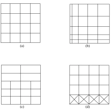
FIGURE 1.1:DIFFERENT TYPES OF MESH TOPOLOGIES;(A) STRUCTURED UNIFORM MESH,(B) STRUCTURED CLUSTERED MESH,(C) UNSTRUCTURED MESH WITH HANGING NODES,
(D) HYBRID MESH ... 5
FIGURE 3.1:AN ARBITRARY MESH TOPOLOGY ... 14
FIGURE 3.2:A FINITE DIFFERENCE STENCIL IN AN ARBITRARY PENTAGONAL CELL ... 16
FIGURE 3.3:MAPPING THE PHYSICAL STENCIL TO A UNIFORM COMPUTATIONAL STENCIL .. 16
FIGURE 3.4:SIMPLE DOMAIN WITH 4 IDENTICAL CELLS ... 20
FIGURE 3.5:DIFFERENT TYPES OF GRID ARRANGEMENT:(A)5X3 GRID,(B)3X5 GRID,(C) 5X5 GRID,(D)9X3 GRID,(E)3X9 GRID,(F) HYBRID GRID ... 24
FIGURE 3.6:EFFECT OF RELAXATION FACTOR FOR CCFD SCHEME,(A)25X25 GRID,(B) 13X49 GRID,(C)49X13 GRID... 26
FIGURE 3.7:COMPARISON OF EXACT ANALYTICAL,PSOR AND CCFD SCHEMES FOR A 25X25 UNIFORM GRID:(A) GRID,(B)CCFD SOLUTION,(C)PSOR SOLUTION,(D) EXACT SOLUTION (K=33),(E) EXACT SOLUTION (K=7) ... 29
FIGURE 3.8:EFFECT OF GRID REFINEMENT ON ERROR DISTRIBUTION:(A)5X5 GRID,(B) 21X21 GRID,(C)49X49 GRID... 29
FIGURE 3.9:CLUSTERED GRIDS TOWARD DIFFERENT BOUNDARIES:(A) BOTTOM CLUSTERED, (B) LEFT CLUSTERED,(C) LEFT CLUSTERED AND GRID REFINED,(D) BOTTOM AND LEFT CLUSTERED ... 31
FIGURE 3.10:CLUSTERING EFFECT:(A)25X25 CLUSTERED GRID,(B)49X25 CLUSTERED GRID,(C)CCFD SOLUTION,(D) EXACT ANALYTICAL SOLUTION (K=33) ... 32
FIGURE 3.11:TWO CELL CENTRES SCHEME ... 33
FIGURE 3.12:TWO END NODES OF THE FACE SCHEME ... 33
FIGURE 3.13:TWO END NODES OF THE FACE AND THE CELL CENTRE SCHEME ... 34
FIGURE 3.14:CONTROL VOLUME SCHEME ... 34
FIGURE 3.16:NODE DISTRIBUTION ALONG THE VERTICAL INTERFACE OF A NON
-CONFORMAL MESH ... 36
FIGURE 3.17:NUMBER OF SEARCHES FOR ONE ITERATION ... 37
FIGURE 3.18:COMPARISON OF FIVE METHODS USED TO CALCULATE THE INTERSECTION VALUES FOR A UNIFORM 13X13 GRID.SOLUTION ALONG HORIZONTAL LINES:(A) Y=0.08333,(B) Y=0.5,(C) Y=0.91667 ... 39
FIGURE 4.1:POISSON BVP ... 41
FIGURE 4.2:CCFD SOLUTION,PSOR SOLUTION, EXACT ANALYTICAL SOLUTION, ABSOLUTE ERROR OF CCFD AND ABSOLUTE ERROR OF PSOR,(A)17X9 GRID, AND (B)17X17 GRID ... 42
FIGURE 4.3:COMBINATION OF DIRICHLET AND NEUMANN BOUNDARIES ... 43
FIGURE 4.4:TYPICAL CELL ADJACENT TO BOTTOM NEUMANN BOUNDARY ... 44
FIGURE 4.5:THREE DIFFERENT METHODS FOR CALCULATING NEUMANN NODES:(A) TWO CELL CENTRE METHOD,(B)2ND ORDER FORWARD DIFFERENCING WITHIN THE CELL, (C)2ND ORDER FORWARD DIFFERENCING WITH TWO NODES ... 45
FIGURE 4.6:RESULTS FOR THREE NEUMANN BOUNDARY NODES IN A 5X5 GRID, COMPARISON OF RESULTS BETWEEN GS AND THREE APPROXIMATION METHODS ... 46
FIGURE 4.7:GRID,CCFD SOLUTION,GS SOLUTION, ABSOLUTE AND RELATIVE DIFFERENCES FOR CCFD VS.GS,(A)25X25 GRID,(B)21X41 GRID ... 48
FIGURE 4.8:CLUSTERED GRID TOWARD ALL BOUNDARIES:(A)25X25 GRID AND ITS SOLUTION,(B)21X41 GRID AND ITS SOLUTION ... 49
FIGURE 4.9:CLUSTERED 21X41 GRID TOWARD THE NEUMANN BOUNDARY:(A) Α =0.99 GRID AND ITS SOLUTION,(B) Α =0.82 GRID AND ITS SOLUTION ... 50
FIGURE 5.1:DIFFERENCING STENCIL FOR (A) VORTICITY,(B) STREAMFUNCTION ... 58
FIGURE 5.2:BACKWARD-FACING STEP DOMAIN AND BOUNDARY CONDITIONS ON PRIMITIVE VARIABLES ... 61
FIGURE 5.3:VELOCITY AND STREAMFUNCTION INLET PROFILES FOR RE =50 ... 63
FIGURE 5.4:STREAMFUNCTION BOUNDARY CONDITIONS ... 63
FIGURE 5.6:REATTACHMENT LENGTH XR ... 66
FIGURE 5.7:REATTACHMENT LENGTH XR AS A FUNCTION OF REYNOLDS NUMBER ... 67
FIGURE 5.8:CCFD GRID SENSITIVITY FOR RE =50 ... 68
FIGURE 5.9:STREAMLINES FOR:(A)RE =50,(B)RE =100,(C)RE =200 ... 69
LIST OF TABLES
TABLE 3.1:CENTRAL NODE VALUES FOR DIFFERENT ASPECT RATIOS AND MESH
REFINEMENTS ... 24
TABLE 3.2:AVERAGE ABSOLUTE ERROR FOR A 25X25 GRID FOR DIFFERENT NUMBER OF TERMS (K) IN THE INFINITE SERIES SOLUTION ... 28
TABLE 4.1:EFFECT OF DIFFERENT GRID SIZES AND RELAXATION FACTORS FOR THE POISSON EQUATION TEST PROBLEM ... 41
TABLE 4.2:AVERAGE ABSOLUTE DIFFERENCE BETWEEN CCFD SOLUTION AND
TRADITIONAL GS SOLUTION FOR DIFFERENT GRID SIZES ... 46
TABLE 4.3:COMPARISON OF ACCURACY OF CCFD RESULTS WITH OTHER NUMERICAL SCHEMES FOR THE CONVECTION-DIFFUSION PDE WITH P=40 ... 52
TABLE 4.4:ABSOLUTE MAXIMUM DIFFERENCE BETWEEN CCFD AND EXACT ANALYTICAL SOLUTION ... 52
TABLE 4.5:CCFD,GS AND ANALYTICAL SOLUTION CONTOURS FOR DIFFERENT VALUES OF P AND Θ ... 53
TABLE 5.1:REATTACHMENT LENGTHS FOR CCFD SCHEME COMPARED TO EXPERIMENTAL DATA AND OTHER NUMERICAL METHODS ... 66
TABLE 5.2:COMPARING THE ACCURACY OF THE CCFD SCHEME ... 67
NOMENCLATURE
relaxation factor (Ch. III)
vorticity (Ch. V)
streamfunction
∆x horizontal spacing
∆y vertical spacing
property (e.g. temperature)
∂ partial derivative
Superscripts
k previous value
k+1 current value
Subscripts
n north intersection
s south intersection
e east intersection
w west intersection
cc cell centre
T top boundary
B bottom boundary
R right boundary
L left boundary
P point or node
CHAPTER I
INTRODUCTION
Finding practical solutions to the governing equations of fluid mechanics is one of the most challenging problems in engineering. These equations, in most cases, form a set
of coupled non-linear partial differential equations (PDEs). In Computational Fluid Dynamics (CFD), the equations of fluid motion are usually approximated by algebraic
expressions using one of several well-established numerical techniques. Currently, the most popular discretization methodologies in CFD are the Finite Difference (FD), Finite Volume (FV) and Finite Element (FE) methods.
The CFD field was dominated by the FD method in its early years. The underlying mathematics that forms the foundation of the FD method is relatively simple.
This allowed researchers to carry out thorough analyses, such as stability and convergence studies, of the algorithms they were developing. Finite difference methods were initially developed for rectangular domains, and CFD researchers found themselves
restricted to flow problems that could be approximated and modeled accordingly. For example, full-potential transonic flow over an airfoil could not be solved because the
flow domain is non-rectangular. However, under the assumption of a thin airfoil which creates only small disturbances to the uniform free stream flow, researchers formulated the so-called transonic small-disturbance theory [1] and were able to obtain good
numerical solutions that assisted engineers to design efficient airfoils for wing cross-sections. During the 1970’s, several researchers developed very sophisticated numerical
simulations [2-4]. However, research is about pushing the envelop, and CFD researchers soon began to place higher demands for the applications of their computer codes, in terms of both the physics that could be modeled and the geometrical complexity of the flow
region. In particular, implementation of the FD formulation is restricted to structured grid systems, i.e. those grid systems that can be organized in such a way that an underlying
logical connection between nodes can be defined. This is a serious limitation in modern-day CFD simulations, since most industrial applications of CFD involve highly complicated geometric structures and passages which cannot be easily or accurately
represented by a structured grid system. Although multiblock methods have been developed to alleviate this problem with the application of the FD method, some issues
still persist, such as complicated computer coding, loss of accuracy across block interfaces and the inability to design a highly automated numerical grid generation process.
In view of the limitation of the FD method to structured grids, extensive research on building new Finite Volume (FV) formulations was started in the late 1970’s. Researchers in solid mechanics had been using the Finite Element (FE) method for many
years and, in the course of their work, had developed fairly sophisticated mesh generation techniques. These mesh systems are referred to as unstructured since there is no logical
connection between nodes in the mesh. Although more difficult to manage in terms of computer logic and storage requirements, unstructured meshes are very popular because of their capability to accurately represent highly complex domains. Furthermore,
FV approach, which can be implemented on either structured or unstructured meshes, has now become central to most of today's commercial CFD codes, such as CFX/ANSYS, FLUENT and STARCD, as well as many research codes. However, the FV formulation
still faces many difficulties, such as those associated with grid arrangement [5]. The pressure-velocity coupling and the correct place to store their values (cell face or cell
centre or a mix of both) constitutes a problem that continues to attract research in FV [6]. Also, high order FV methods cannot easily be formulated or implemented.
A new FD approach is presented in this thesis, which has the flexibility to be
applied on an unstructured mesh. The governing equations are differenced over all the cell centres (control volume centres) instead of the grid points as would typically be done
in a conventional FD approach, and hence the name Cell-Centred Finite Difference (CCFD). The nodes are then updated by averaging the property from all the cell centres that share that node.
Several simple test cases are investigated in this thesis to illustrate the development and application of this new method. The numerical results are compared with analytical solutions if available and/or traditional FD solutions. Even in many
simple instances the analytical solution is not available, perhaps being restricted due to the boundary condition type. For example, an elliptic equation subject to Dirichlet
boundary conditions (i.e. boundary values are specified) may have an analytical solution. However, the same equation subject to a Neumann boundary condition (i.e. normal derivative of the variable is specified) may not have an analytical solution. At the same
needed to map the clustered grid points in the physical domain to a set of equally spaced grid points in the computational domain.
When the solution domain can be discretized to a structured grid with uniform
spacing, as shown in Fig. 1.1a, traditional FD is more efficient than either FV or FE, i.e. it is more stable and needs less resources. However, for curvilinear coordinates or
unequally spaced grid lines, as in Fig. 1.1b, the physical domain must be transformed to a computational domain, where the PDEs are solved after also being transformed. In the case of complex geometries and when hanging nodes exist (e.g. interior nodes that have
three cells around it instead of four), as illustrated in Fig. 1.1c, the traditional FD method must be designed as a multiblock scheme. The traditional FD method cannot handle a
mesh topology such as the one shown in Fig. 1.1d, while FV and FE have the ability to handle all the mesh topologies shown in Fig. 1.1.
The overall objective of this thesis research is to develop a finite difference based
scheme for solving partial differential equations which can be implemented on both structured and unstructured mesh systems. The CCFD method developed in this research is designed to be applicable to any physical problem that can be mathematically modeled
by PDEs with associated initial and/or boundary conditions. At each step in the development, a simple question is asked: “Does this assumption, or derivation, or
decision restrict the general applicability of the method?”. Although this thesis concentrates on the development of the CCFD method for 2-dimensional problems, it is anticipated that, in future research, this method will be extended to 3-dimensional
(a) (b)
(c) (d)
CHAPTER II
REVIEW OF LITERATURE 2.1 Introduction
There is a vast body of literature that discusses issues regarding the numerical
solution of partial differential equations. Likewise, the literature on the numerical simulation of fluid flows is extensive. Although there has been much research in these fields, most of it does not directly impact on the research presented in this thesis. Rather,
some fundamental ideas developed over many decades of research have informed the formulation of the Cell-Centred Finite Difference (CCFD) method. In this chapter, some specific literature that is relevant to the research in this thesis is reviewed.
2.2 Classical Numerical Schemes in CFD
Peiro and Sherwin [7] have presented the fundamental concepts of the FD, FV
and FE methods. They point out that the integral formulation (i.e. FV and FE formulations) of the governing equations is more advantageous since it handles Neumann
boundary conditions and discontinuous source terms in a more natural way. Moreover, the integral form deals with complex geometries better than the differential form (i.e. FD) as it doesn't rely on the type of the mesh, i.e. the mesh can be structured, unstructured or
hybrid. The rules for assignment of weighting functions and the similarity between FV and FE discretization strategies are explained by Mattiussi [8]. Onata and Idelsohn [9]
The fundamental concepts of FV and details of FD formulas are explained by Hoffmann and Chiang [10, 11], Smith [12], and in many other CFD textbooks. The main differences between the three classical numerical schemes include the following points.
FD and FV generate the discretized equation at any node based on the corresponding values at neighbouring nodes. In the FE method, the discretized equation of each element
is independent of the other elements. In FE, incorporating different types of boundaries (i.e. Dirichlet and Neumann) is simpler, because it will only effect the element equations. On the other hand, FD and FV formulations need to be modified for derivative
boundaries. In FD and FV the coupling between the discretized equation setup and its solution is based on the cell type, while in FE, adding new cell types will only change the
local cell equations and the final solution procedure through the global matrices doesn't need to be modified. In the CCFD formulation developed in this thesis, each cell is considered in much the same fashion as in the FE method. The effect of cell type and its
geometrical details is translated into constant coefficients in the FD equation for that individual cell. However, unlike FE, in CCFD the global matrices do not need to be assembled, and the cell-centre values of adjacent cells are linked through the updating
procedure of the physical mesh nodes. This part of the procedure is closer to techniques commonly used in FV formulations.
Gottlieb and Orzag [13] and Saleh [14] explain another method to solve differential equations through approximating the unknown functions by using Fourier series or a series of Chebyshev polynomials, which is known as the Spectral Method.
and FE methods is that the series is valid throughout the domain, whereas the solution is local in the mesh-based methods. Similarly, as implied by the name, meshless methods do not require a grid on which to discretize the governing equations.
2.3 Locating Variables and Related Issues in FV Method
As described by Patankar [16], who is regarded as one of the primary authors of
the Finite Volume method, if pressure and velocity components of an incompressible fluid flow are stored in the same location (i.e. non-staggered or collocated grid), an
oscillatory or "checkerboard" pressure field may occur. To avoid this problem, researchers developed the idea of a staggered grid, in which each of the flow variables is calculated and stored at a different node in the mesh [16]. In this type of grid system, the
pressure-velocity coupling is usually handled through some variation of the SIMPLE algorithm [16], or by formulating a Poisson equation for pressure that simultaneously
ensures that mass is conserved [10]. Generally speaking, staggered grids will be structured, so it is also possible to employ this type of grid system in a FD formulation. In a recent research conducted by Barron and Zogheib [17], a new numerical algorithm was
developed for solving 2D incompressible flow equations on a staggered curvilinear grid by replacing some weaknesses in FD with equivalent strong parts of FV, especially the
velocity-pressure coupling. One of the significant advantages of the FD approach in [17] is that it avoids the need to calculate fluxes at the cell faces, which is central to all FV formulations.
advantages associated with calculating all variables at the same location, researchers have devised schemes to solve the resulting non-realistic pressure fields. Rhie and Chow [19] performed a numerical study on 2D, incompressible, steady flow. They developed a
“momentum interpolation” scheme on an ordinary (non-staggered) grid to suppress the pressure oscillations by adding a pressure gradient term into the pressure interpolation.
Reggio and Camarero [20] developed a scheme that employs upwind differencing for the velocity gradients and downwind differencing for the pressure gradients to prevent the odd-even pressure field. In another research, Thiart [21] presented a differencing scheme
that accounts for the effect of pressure on the velocity gradients. Peric et al. [5] and Demirdzic et al. [22] did a comparison between a staggered and a collocated grid
arrangement for three test cases, and they indicated the advantages of a collocated scheme in terms of convergence speed and the ability to extend the implementation to non-orthogonal grids. Versteeg and Malalasekera [23] have also explained the issues
related with the FV formulation on a curvilinear body-fitted structured grid, and the need for special correction expressions for the diffusion and convection fluxes in an unstructured grid. They have presented a special pressure-velocity coupling on a
collocated grid which avoids the checkerboard pressure effect. They emphasize on the pressure interpolation practice developed in [19] and its success in collocated curvilinear
body-fitted and unstructured grids. Majumdar [24] demonstrated the dependency of the momentum interpolation scheme on the under-relaxation factor, and proposed a new scheme for calculating the velocity value at cell faces which preserves a convergent
To maintain the advantageous features of a collocated grid, in this thesis a FD scheme is developed that locates or stores all the variables at the same location, the cell centre. A combination of the non-staggered FV philosophy with robust FD
approximations is observed, and since it is a purely FD formulation, there is no need for approximating the fluxes across cell faces.
Other endeavors to develop a FD formulation similar to the CCFD formulation, at least in terms of confining the flow variables to the cell centre, can be seen in the MHD (Magneto-Hydro-Dynamics) field, as presented by Livne et al. [25], Stone and Mihalas
[26], Gardiner and Stone [27], Mignone et al. [28] and Spekreijse [29]. Spekreijse [29] uses differencing stencils comprised of four cells, and shows that a nine-point 2D upwind
stencil changes into a five-point block stencil. Other than the fact that these works are “cell-centred”, they shared very little common features with the current CCFD method developed in this thesis.
2.4 Model Equation
Several benchmark test cases for incompressible flows can be found in the
literature (eg. cf. [30] and [31]). New types of FV formulations are verified using these benchmark problems [32, 33]. In recent research, a detailed comparison between
node-centred and cell-node-centred FV formulations was conducted by Diskin et al. [6]. Using the Poisson equation as their model equation, six second-order schemes were developed for six typical regular and irregular grids. They found that grid skewness plays a critical role
Maintaining a stable solution with a higher order of accuracy has always been one of the main objectives of new numerical methodologies. Sakai and Watabe [34] have proposed a new trial to increase the accuracy of numerical fluxes in the case of advection-diffusion
equations. This further supports the conflicting issues in CFD and the motivation to re-assess the entire CFD approach.
2.5 Accelerating the Solution
The process of solving a physical engineering problem starts with defining the
PDEs that model the problem. Then the PDEs are discretized, and the resulting algebraic equations, which can be assembled into a matrix equation, are solved over a discrete set of mesh points. For this purpose, direct and indirect/iterative methods are used. Iterative
methods are more common in CFD because the matrices are very large and often have a well-defined sparse structure, and since iterative methods need less computational
resources. It is well-known that using a so-called relaxation factor improves the
convergence rate [10]. The effect of relaxation can be thought of as the addition of only a portion of the residuals, which is the difference in value between two successive
iterations, to the calculated value for any node. In another words, it squeezes the gap between the initial and final solution faster. This influence is maximum at the first iterations and reduces as the solution approaches its final state within the pre-defined
convergence criterion. There are no general directions for calculating the optimum
value. Although can be calculated for some applications, it will be limited to
specific details like domain geometry and boundary type. Based on the relaxation
over-relaxed (1 2 or the basic Gauss-Seidel ( 1). In most cases the value of
increases with finer meshes. Versteeg and Malalasekera [23] state that is mesh
dependent and no guidelines exist for exact value computation. Attempts to set up a numerical formulation that doesn't rely on a relaxation parameter have been conducted,
like the work of Majumdar [24]. However, current CFD simulations still rely heavily on the idea that relaxation can provide accurate and stable solutions over a wide range of
applications.
2.6 Thesis Objectives
In this thesis, the CCFD approach reveals new vistas for research across the whole scope of CFD. A new FD scheme is presented for structured grid systems, with the flexibility to be extended to unstructured grids. As in all fundamental research in CFD, to
introduce a new differencing scheme, a single PDE is used, e.g. [31]. The 2D Laplace equation is considered as the model equation in this study,
0 (2.1)
with Dirichlet and/or Neumann boundary conditions. To develop and explain the method, the mesh is initially constructed with rectangular cells of uniform size. The FD scheme is derived from the differential form of the conservation laws.
The thesis is organized as follows. The basic formulation of the CCFD method is described in Chapter III. Many of the critical aspects of any useful numerical method are
out in Chapter IV, where the CCFD method is applied to a Poisson equation with Dirichlet boundary conditions, a Laplace equation with Neumann boundary conditions, and a model convection-diffusion equation with Dirichlet conditions. The CCFD method
is then applied to a benchmark incompressible fluid flow problem, that is, the flow over a backward-facing step, in Chapter V. Chapter VI includes the conclusions from this
CHAPTER III
DESIGN AND METHODOLOGY 3.1 The CCFD Scheme
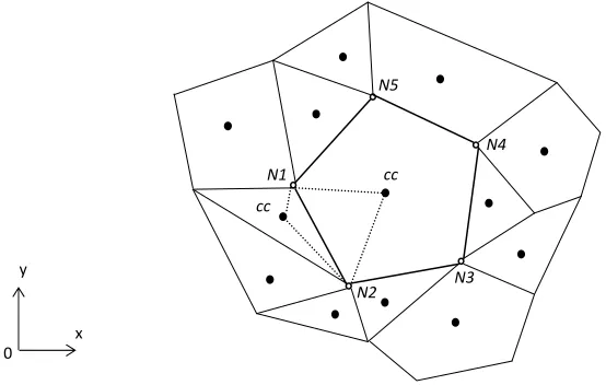
Consider an arbitrary polygonal cell in 2D bounded by the line segments joining
nodes N1, N2, N3, N4 and N5, surrounded by neighbouring cells as shown in Fig. 3.1.
Figure 3.1: An arbitrary mesh topology
The coordinates of nodes N1,…,N5 with respect to a fixed global Cartesian coordinate system Oxy are assumed to be known. An arrangement of nodes such as shown in Fig. 3.1 does not allow for a traditional FD formulation of the governing PDE
since there is no orderly pattern to the placement of nodes. Traditional FD methods
requires that all nodes (grid points) lie at the intersection of lines and .
On the other hand, the FV and FE methods can be implemented on polygonal cells. For these methods, the governing PDE is first reformulated as an integral equation by performing a double integration of the PDE over the region contained within the cell.
In the cell-centred FV method, the double integral is then converted into a line integral around the boundary of the cell using Green's theorem. This line integral is written as the
0
y
x
cc
cc N5
N4
N3 N2
sum of line integrals along the straight lines joining the nodes, i.e. along the faces (or edges) of the cell. For example, consider the line integral along the face joining nodes N1
and N2. To evaluate the integral exactly we need to know the variation of (or perhaps
or ) along the face. Since this variation is unknown (otherwise we would already
know the solution to the original PDE), it must be approximated. A simple approximation
would be to take to be constant along the face, with value as the average of at the two
end nodes N1 and N2. Alternatively, we could approximate using the cell-centre values
of the two cells sharing the face joining N1 and N2. Applying this procedure to all cells in the domain, one can formulate a system of algebraic equations for the values of at all
cell centres. This system is then solved, either by direct or iterative matrix solvers. If
nodal values are required, e.g. at node N1, it can be obtained by taking a distance weighted average of cell-centre values for all cells sharing node N1.
In the FE method, the integrand is approximated over the cell, and then the double
integration is performed exactly. The approximation will involve the unknown values of
at the nodes of the cell, and must be a function which is integrable over the cell area. Assembling the equations obtained from each cell will lead to an algebraic system of
equations for the unknown nodal values.
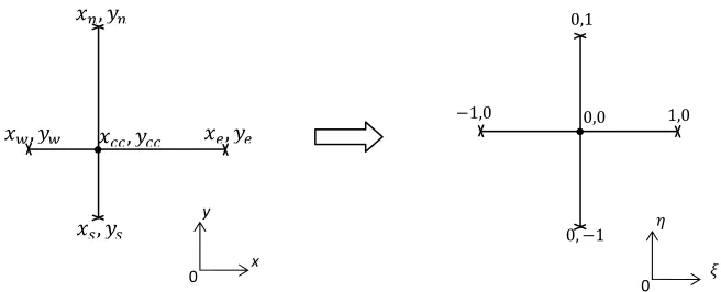
In the CCFD method, the PDE is applied at the centre of each cell, and the partial
derivatives in the PDE are approximated by finite differences. To accomplish this, a finite difference stencil is placed inside the cell, with the centre of the stencil located at the centroid of the cell, as illustrated in Fig. 3.2. The arms of the stencil are positioned to be
denoted by w, e, n and s. Standard finite difference formulae require uniform spacing between grid points, or, in the present context, that the distance from s to cc equals that from cc to n. Clearly, for an arbitrary cell topology, this will not be the case.
Figure 3.2: A finite difference stencil in an arbitrary pentagonal cell
One option would be to use finite difference approximations that account for variable grid spacing, but this degrades the accuracy of the approximation. A better
approach, which preserves the accuracy of the standard formulae, is to map the non-uniform stencil to a non-uniform one, as demonstrated in Fig. 3.3.
Figure 3.3: Mapping the physical stencil to a uniform computational stencil
, ,
, ,
,
0
y
x
0, 1 0,0
1,0 1,0
0,1
0
cc N5
N4
N3
The line segment joining w to e is mapped to 1 1, with cc mapped to
0. Similarly, the stencil arm joining s to n is mapped to 1 1, with cc mapped
to 0. These mappings can be expressed as quadratic functions:
(3.1)
Denoting the coordinates (with respect to the global system) of w by ( , ),
coordinates of e by ( , ), etc., it can be shown that the coefficients in (3.1) are given
by:
, ,
(3.2)
, ,
Standard finite difference formulae can be used in the ( , ) system, in which
Δ 1, Δ 1. To apply these standard approximations, the governing PDE must also
be transformed to the ( , ) coordinates. Using chain rules, we get, for example,
1
(3.3)
1 1 1
and similarly for , and higher order derivatives. In these expressions the metrics
are given by 2 and 2 . Since the partial derivatives are
locally approximated at the cell centre, x', x'', y' and y'' are evaluated at 0, 0.
Therefore, , 2 , and 2 . Using eqn. (3.2), the metrics
, 2
(3.4)
, 2
Note that the values of the metrics are cell specific. The governing PDE is not globally
transformed under eqn. (3.1). It is uniquely transformed for each individual cell.
To illustrate the fundamental concepts of the CCFD method, consider the Laplace
equation:
0 (3.5)
Using transformation (3.1) and the relationships (3.3), the Laplace equation in the , coordinates becomes:
1 1
0 (3.6)
where x', x'', y' and y'' are given by eqn. (3.4). Now, suppose three-point central differencing is used to approximate the derivatives in eqn. (3.6), i.e.
2 , 1
2
(3.7)
2 , 1
2
Applying the approximations (3.7) to the eqn. (3.6), the resulting finite difference
equation can be written as,
(3.8)
where 1 1
,
,
Following procedures similar to those used in the FV method, the values of ,
, and can be approximated in terms of cell nodal values and neighbouring cell
centroid values. Equations for the nodal values can be constructed using the distance weighted average of cell-centre values for all cells sharing the node. Assembling the resulting equations at all cell centroids and all nodes leads to a system of linear algebraic
equations which can be solved by standard numerical procedures.
In this thesis, rather than assemble the large matrix system, we use an iterative
approach. An initial guess for at all cell centroids and nodes is made. A particular node
P is selected and all cells sharing that node are identified. Then, for each of these cells,
, , and are evaluated based on the initial guess. Equation (3.8) is used to
update the value of for each of the cells. The value of at the selected node P is then
updated using
∑
∑ 1 (3.9)
where is the number of cells sharing node P, cc1, ... , are the centroids of these
cells and is the distance from centroid to the node P.
The next node is selected and the above procedure is followed to update the nodal value, until all nodes in the mesh have been updated, completing the first iteration. The
3.2 A Simple Test Problem
A simple test problem is chosen to demonstrate how the CCFD method is implemented. Consider the solution of the Laplace equation (3.5) on a square domain
with four square cells, as shown in Fig. 3.4. The domain size is 1 unit by 1 unit, with equal grid spacing (∆x = ∆y). Dirichlet conditions are applied, with all boundaries set to
be zero except for the left boundary, which is taken to have the value 1.
Figure 3.4: Simple domain with 4 identical cells
3.2.1 Solution procedure
In this example, the only node to be evaluated is the domain central node (P). The general procedure is as follows:
a. find the cells that share the current node (i.e. node P)
b. for each one of these cells;
i. calculate the cc coordinates, and the coordinates of w, s, e and n
intersections.
ii. calculate e by distance weighted averaging between the two centres of the
Similarly, evaluate n, w and s. If the intersection lies on a boundary, use
the corresponding boundary value.
iii. evaluate cc from the discretized FD form of the model equation. Second
order central differencing is used, leading to eqn. (3.8).
c. update node P by a distance weighted averaging from all adjacent cell centres,
using eqn. (3.9).
The calculations start with an initial guess at P and all the cell centres, which are then updated iteratively until the convergence criterion is satisfied.
For the domain shown in Fig. 3.4, using the CCFD formulation with successive
over-relaxation and a relative difference between iterates of 10E-9, P was found to be
0.25 after 7 iterations ( = 1.413). This is in excellent agreement with the exact
analytical value of 0.25. The analytical solution for this test problem can be found in many resources, and is given by:
, lim 4 (3.10)
where L is the left boundary value, L and H are the length and the height of the domain,
K is the number of terms in the summation and (x, y) are the Cartesian coordinates of any internal point in the domain (not necessarily a node).
For each cell in the CCFD formulation, the property value of the north, east, south
boundary or an internal one. This may occur in an unstructured grid with triangular cells, or a hybrid mesh (see Fig. 3.5f). Alternatively, the intersection may lie on a boundary face (a face is a line that joins two nodes). In this case the boundary value is directly
assigned to the intersection, e.g. w = 1 for cell number one in Fig. 3.4. This means that
the second part of Step b of the solution procedure is only applied when the intersection lies on an internal face, and is modified otherwise as explained above.
For square cells, instead of using the two adjacent cell centres, the intersection values can also be calculated by a distance weighted average between the two nodes
forming the face on which the intersection lies. In this case, the differencing stencil incorporates the property values at the corners of the cell. This is equivalent to a nine-point formula of FV and FE which is derived in [8]. In other words, the CCFD scheme
uses four "corner" values, while the traditional FD formulation does not. Other methods of calculating the intersection values are explained in section 3.4 of this chapter.
3.2.2 Mesh refinement and solution relaxation
With the same domain size and boundary conditions mentioned above in section
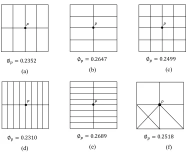
3.2, several types of (uniform) grid refinements and cell arrangements have been tested, without clustering. The grid arrangements and results for the domain central node value
are shown in Figs. 3.5a-f. For cell aspect ratio ( = ∆x/∆y) not equal to 1, i.e. non-square
cells, the accuracy of the solution is reduced for coarse grids. This decrease in accuracy is also observed with traditional FD solutions for the same grids. Figures 3.5a and 3.5d show the results of refinement in the x-direction, corresponding to cell aspect ratios less
than 1, i.e, = 0.5 and 0.25, respectively. In both cases, the value of P is less than the
heavily influenced by the boundary conditions on the right, bottom and top of the domain (all zeros). The non-zero value on the left boundary, which drives the solution away from zero, only influences the solution through one node on the left boundary. The exact
solution can be recovered by inserting additional nodes on the left boundary, as shown in Fig. 3.5c. The reverse occurs when the cell aspect ratio is taken greater than 1, as
illustrated in Figs. 3.5b and 3.5e, where the non-zero left boundary dominates the solution. However, with CCFD, for any value of , grid refinement improves the
solution. Some typical results are tabulated in Table 3.1. M and N are the number of grid
points in the x- and y-directions, respectively.
For a hybrid mesh (a mix of two different cell types in one domain), as shown in
Fig. 3.5f, P was found to be 0.2518. It should be mentioned here that eqns. (3.8) and
(3.9) are solved for the property value at the cell centres and nodes respectively. This case provides a counterexample to the widely-held argument (cf., e.g. [6]), that the bottleneck of the FD formulation is that it cannot handle an unstructured mesh system
over a complex geometry, because it requires a topologically square network of lines to discretize the PDEs. In fact, the present CCFD scheme is able to handle an arbitrary unstructured mesh made up of triangular cells or a hybrid mesh comprised of both
0.2518 P
(a) (b) (c)
(d) (e) (f)
Figure 3.5: Different types of grid arrangement: (a) 5x3 grid, (b) 3x5 grid, (c) 5x5 grid, (d) 9x3 grid, (e) 3x9 grid, (f) hybrid grid
Table 3.1: Central node values for different aspect ratios and mesh refinements
β MxN фP iter
0.25 9x3 0.2310 63
0.25 49x13 0.2494 551
0.5 5x3 0.2353 20
0.5 25x13 0.2495 175
1 3x3 0.2500 7
1 13x13 0.2500 94
2 3x5 0.2647 16
2 13x25 0.2505 281
4 3x9 0.2690 63
4 13x49 0.2506 955
P
0.2352
P
0.2647
0.2689 P
0.2310 P
Table 3.1 indicates that a finer mesh recovers the loss in accuracy created by non-square cells, although more computation time will be associated with the higher number of cells. In this case, an accelerated solution will be desired for the iterative solver.
Hoffmann and Chiang [10] state that introducing a relaxation factor into the discrete
form of the FD approximation of the PDE should accelerate the solution (i.e. reduce the
number of iterations), provided that 1 ≤ ≤ 2. In the current research, several grids (with
rectangular cells) have been tested with a relaxed form of the CCFD scheme, which is expressed as:
(3.11)
where n+1 and n are the current and the previous iteration indices respectively, and the
tilda indicates the cell-centre value calculated from eqn. (3.8).
CCFD results for two grid systems are shown in Fig. 3.6, illustrating the relationship between the number of iterations required for convergence and the value of
the relaxation factor. The optimum value for the relaxation factor was found to be 2.56 and 1.99 for 25x25 and 13x49 grid sizes respectively.
(a)
0 200 400 600 800 1000
iter
omega
(b)
(c)
Figure 3.6: Effect of relaxation factor for CCFD scheme, (a) 25x25 grid, (b) 13x49 grid, (c) 49x13 grid
3.3 Solution of Test Problem
3.3.1 Uniform grid
A 25x25 grid has been selected to check many of the important aspects of the iterative numerical solution (optimum relaxation factor, number of iterations, average
absolute error, etc.). A comparison between the exact analytical solution (eqn. (3.10)), the CCFD solution and a traditional FD point successive over-relaxation (PSOR) solution is
0 200 400 600 800 1000 1200 1400 1600 1800 iter omega iter 0 1000 2000 3000 4000 5000 6000 7000 8000 9000 10000
1.50 1.63 1.75 1.88 2.00 2.13 2.25 2.38 2.50 2.63 2.75 2.88 3.00
iter
omega
shown in Fig. 3.7. A relative difference between iterations is used for the convergence criterion, with tolerance less than or equal to 10E-9 at each node, for both the CCFD and PSOR solutions. The equations used for the PSOR scheme can be found in [10] (p.164,
eqns. (5-18) through (5-20)). The optimum relaxation factor for the PSOR scheme was found to be 1.769, which made the solution converge after 86 iterations, while the
optimum relaxation factor for the CCFD scheme was found to be 2.56 (in a tested range of 1.0 to 2.7) with 340 iterations to converge (see Fig. 3.6a). For most of the grid sizes
that were tested, choosing beyond this range (1.0 to 2.7) leads to a sudden large
increase in the number of iterations, as seen in Fig. 3.6c, or even divergence in some cases.
In the FV method, under-relaxation is normally used to control the oscillations in
an iterative solution of this problem. Majumdar [24] proposed a FV formulation for calculating the velocity value at cell faces which preserves a convergent solution, independent of the under-relaxation factor and without significant increases in
computational time. In another word, trials were made to untie available FV formulations
with the classical relaxation bounds, i.e. (0 < < 1). Such a decoupling may be possible in the CCFD method, but has not been explored in this thesis.
The average absolute error (for both CCFD and PSOR) over all the interior nodes is the difference between the numerical and exact analytical solution. However the
“accuracy” of the exact solution itself, which is calculated from eqn. (3.10), depends on the number of terms (K) that are included in the summation. Figures 3.7d and 3.7e show the effect of a high or low number of terms. This leads to variations in the average error
number of terms in the exact solution (i.e. in eq. (3.10)) without any modification to the grid. Naturally, the higher number of terms (K) in a relatively fine mesh (e.g. 49x49) is associated with increasing the processing time. However, most importantly, this example
demonstrates that the CCFD method provides a solution with the same level of accuracy as the traditional FD method.
Table 3.2: Average absolute error for a 25x25 grid for different number of terms (K) in the infinite series solution
K CCFD PSOR
7 0.00215 0.00215 11 0.00098 0.00098 33 0.00041 0.00041
(c) (d)
(e)
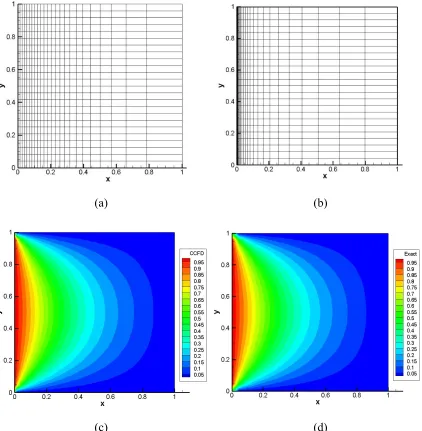
Figure 3.7: Comparison of exact analytical, PSOR and CCFD schemes for a 25x25 uniform grid: (a) grid, (b) CCFD solution, (c) PSOR solution, (d) exact solution (K = 33),
(e) exact solution (K = 7)
The effect of grid refinement on the solution accuracy is shown Fig. 3.8. Three structured grids are used for this purpose.
Abs. Err.
Rel. Err.
(a) (b) (c)
3.3.2 Clustered grid
To explore the effect of clustering grid lines toward different directions, first
some simple cases of clustering are considered on coarse grids, then finer grids are considered. Again, the same domain size and boundary conditions mentioned in section 3.2 will be utilized. Figures 3.9a and 3.9b show the addition of nodes toward the bottom
and the left boundaries, respectively. One may expect that adding nodes close to the left boundary would make the results more accurate, but this is not the case for coarse grids.
To understand the reason for this, note that in Fig. 3.9a, two nodes lay on the left boundary, which is the non-zero boundary, and four nodes fall on the other three zero
boundaries, giving a ratio of two to four, and a reasonably accurate solution P = 0.2570.
On the other hand, in Fig. 3.9b the same ratio of nodes is one to five, and the solution P
= 0.2230 is considerably less accurate. Comparing Fig. 3.9b and 3.9c makes the scope more clear, where the ratio of non-zero to zero boundary nodes is changed from 1 by 5 to
3 by 7, which brings the value of P from 0.2230 to 0.2522. In another word, the number
of nodes on any boundary reflects the effect of that boundary on interior nodes, implying that the number of grid points in each direction must be chosen so that all boundaries
sufficiently influence the interior solution. However, this significant effect is true for coarse grids, and may or may not have the same impact in fine or dense grids.
With the grid clustered toward the left boundary, as shown in Figs. 3.10a and
3.10b, the CCFD method shows a close match with the analytical solution (see Figs. 3.10c and 3.10d). Two types of clustering procedures were used to design these grid
(Fig. 3.10b). Packing the grid to the left boundary using a scale factor α means that the ratio of adjacent cell lengths is α, i.e. ∆xi-1 = α∆xi.
(a) (b) (c)
(d)
Figure 3.9: Clustered grids toward different boundaries: (a) bottom clustered, (b) left clustered, (c) left clustered and grid refined, (d) bottom and left clustered
The grid in Fig. 3.10b, which exhibits tight packing at the left boundary, was
generated with α = 0.8. For some of these types of grids, the cell aspect ratio gets extremely small (β < 0.00014 for the 49x25 grid in Fig. 3.10b). Although most other
numerical solution schemes have difficulty dealing with small (or large) aspect ratios, it is interesting to observe that the CCFD scheme can handle this extremely small aspect ratio, and produces a highly accurate solution. In this example, clustering also leads to an
increase in the number of iterations for the CCFD scheme, from 340 iterations for the
uniform grid with = 2.56, to 372 iterations for the clustered grid with the same
relaxation factor.
P
0.2570
P
0.2522
P
0.2384 0.2230
(a) (b)
(c) (d)
Figure 3.10: Clustering effect: (a) 25x25 clustered grid, (b) 49x25 clustered grid, (c) CCFD solution, (d) exact analytical solution (K = 33)
3.4 Alternative Methods to Calculate Intersection Values
There are other methods to calculate the property value at the four intersections (n, s, e and w) from cell centres and/or nodes. All of the ones discussed below involve
intersection. We illustrate these procedures by considering the evaluation of the east (e) intersection point in a cell.
3.4.1 Two cell centres
Figure 3.11: Two cell centres scheme
1
1 1
1
(3.12)
where | | and 1 | |.
3.4.2 Two end points (nodes) of the face
Figure 3.12: Two end nodes of the face scheme
1 2
1 1 12
(3.13)
where 1 | | and 2 | |.
N1
N2 L2 e
L1
cc
e L1 L
3.4.3 Two end nodes of the face and the cell centre
Figure 3.13: Two end nodes of the face and the cell centre scheme
1 2
1
1 12 1
(3.14)
where | |, 1 | | and 2 | |.
3.4.4 Control volume
In this case, we construct a control volume from the two face end points (nodes), the current cell centre and the centre of the cell adjacent to the east face.
Figure 3.14: Control volume scheme
1 2 3
1 1
1 12 13
where | |, 1 | |, 2 | | and
3 | |.
3.4.5 Four vertices of the cell
Figure 3.15: Four vertices scheme
where 1 | |, 2 | |,
3
and 4
Schemes 3.4.2, 3.4.3 and 3.4.5 are more relevant to the core of the CCFD formulation, starting from the name CCFD, i.e. all the necessary information for the
numerical evaluation of the calculated property at the cell centre comes from the current cell nodes and/or centre. This feature adheres to an important principle in the development of the CCFD method, to treat an unstructured mesh with its simplest
formulation. In this context, simplest refers to two significant issues in the numerical solution of PDEs that govern physical processes. First, these schemes give more
1 2 3 4
1
1 12 13 14
(3.16)
L4 L3 N3
N4
e N1
flexibility to CCFD to handle an arbitrary number of cells and types that may share a single node. Also, it allows the CCFD method to handle cells that possess a number of nodes greater than its physical nodes at the cell vertices. These are commonly referred to
as hanging nodes and occur on the two layers of cells that lay on the interface of a non-conformal mesh, as illustrated in Fig. 3.16.
Figure 3.16: Node distribution along the vertical interface of a non-conformal mesh
Secondly, these schemes permit easier programming because no information from neighbour cells is needed. In the cases where data is needed from out of the cell, like the
two cell centres method, the neighbouring cells should be identified. This can be done out of the solver part of the program, i.e. in the geometry part, in which case more computer memory is claimed. Alternatively, if it is kept within the PDE solver, then extensive
processing time is required with larger meshes. The extra processing time originates from the searching process for the second cell that shares the same couple of nodes with the
imagine the size of searching, consider a structured grid of square cells with 49 by 49 nodes. Then,
No. of internal nodes = (49-2) X (49-2) = 2209
No. of cells to be evaluated = (No. of internal nodes) X (No. of cells adjacent to each node) = 2209 X 4 = 8836
No. of searches = (No. of cells to be evaluated) X (No. of intersections for each cell)
= 8836 X 4 = 35344
To illustrate this further, see Fig. 3.17 which shows the exponential increase in the
number of searches as the number of internal mesh points increase.
Figure 3.17: Number of searches for one iteration
A grid of 13x13 nodes was selected to compare the results of these five methods for evaluating the intersections values. The boundary value problem described in section 3.2
has been solved using each of these five schemes. For comparison to the exact solution,
0 10000 20000 30000 40000 50000 60000 70000 80000 90000
5X5
11X11 25X25 35X35 49X49 75X75
No. of
Searches
grid size (MXN)
three horizontal rows of grid points (nodes) are selected. These three rows are: the second row of nodes from the lower boundary (y = 0.08333), in the middle of the domain (y = 0.5), and the second row of nodes from the top boundary (y = 0.91667). Property values
from the left to the right boundary along these three rakes are shown in Fig. 3.18. For a uniform grid, corresponding to the data presented in Fig. 3.18, these graphs show that all
five schemes have good accuracy (compared with the exact solution). However, further simulation tests have shown that, for grid systems with high and low cell aspect ratios, the two cell centres, two nodes and control volume schemes were more accurate than the
other two schemes. As for convergence speed, the two cell centres scheme was always the fastest (i.e. converged with less number of iterations) compared with rest of the
schemes. For this reason, the two cell centres scheme will be used to calculate the intersection values for all the problems in Chapter IV and Chapter V.
(a)
0 0.2 0.4 0.6 0.8 1 1.2
Nodal
val
ues
x-coord
(b)
(c)
Figure 3.18: Comparison of five methods used to calculate the intersection values for a uniform 13x13 grid. Solution along horizontal lines: (a) y=0.08333, (b) y=0.5, (c)
CHAPTER IV
ANALYSIS OF FURTHER VERIFICATION TESTS
4.1 Introduction
In this chapter the CCFD method is implemented on three additional test problems that have been investigated by other researchers using other numerical methodologies. These three test cases are meant to explore the extendibility of the
proposed CCFD scheme to other types of PDEs and boundary conditions. The investigations that have been reported in Chapter III are not all repeated for each problem. However, some aspects will be summarized in tables and/or presented in
contour plots.
4.2 Poisson's Equation with Dirichlet Boundaries
Winslow [35] used Poisson's equation to test and explain a new numerical scheme over a triangle mesh. Therefore, to further test the CCFD method, a boundary value problem for the Poisson equation has been selected from [36]. The domain is a 1 unit x
0.5 unit rectangle, subject to a variable Dirichlet condition at the bottom boundary, and constant Dirichlet conditions on the rest of the boundaries. The PDE to be solved is
2 1 (4.1)
with solution domain and boundary conditions as illustrated in Fig. 4.1. This boundary value problem has an exact analytical solution which is also provided in [36], given by
Figure 4.1: Poisson BVP
All the parameters and solution aspects investigated for the first test case in
sections 3.2 and 3.3 can also be applied to this case. However, only the effects of grid refinement and relaxation factor are shown in Table 4.1. This problem has an exact
analytical solution given by eqn. (4.2) and therefore both CCFD and PSOR (traditional FD method) solutions can be compared to the analytical solution. The last two pairs of columns in Table 4.1, absolute maximum error and relative maximum error, show that for
all the tested grids, CCFD is more accurate than the traditional PSOR. As for the number of iterations, with the same convergence criterion, CCFD needs more iterations to
converge.
Table 4.1: Effect of different grid sizes and relaxation factors for the Poisson equation test problem
MxN Num. of Iter. Omega Opt AbsMaxErr RelMaxErr CCFD PSOR CCFD PSOR CCFD PSOR CCFD PSOR 5x3 12 8 1.575 1.033 0.04930 0.07856 0.4161 0.8562 5x5 17 14 1.825 1.172 0.04822 0.07922 0.4706 1.1841 9x5 23 19 2.075 1.267 0.04248 0.07980 0.4368 1.3560 9x9 54 28 2.200 1.447 0.04297 0.08051 0.4492 1.4653 17x9 67 37 2.450 1.533 0.04111 0.08067 0.4526 1.5987 17x17 193 56 2.200 1.674 0.04155 0.08187 0.4555 1.6282
0
0 0
CCFD
PSOR
Exact
AbErCC
AbErSOR
(a) (b)
Figure 4.2: CCFD solution, PSOR solution, exact analytical solution, absolute error of CCFD and absolute error of PSOR, (a) 17x9 grid, and (b) 17x17 grid
degree of accuracy than the traditional FD method. This conclusion is typical of other grid arrangements applied to this BVP.
4.3 A Combination of Dirichlet and Neumann Boundaries
A worked example from [37] has been selected to further verify the CCFD scheme. In this example, the governing PDE is the Laplace equation and the solution
domain has a derivative (Neumann) condition at the bottom boundary, while the rest of the boundaries are Dirichlet. Since there is no analytical solution available for this
particular example, the CCFD solution will be compared with the PSOR (traditional FD) solution. Figure 4.3 shows the problem domain and boundary conditions.
Figure 4.3: Combination of Dirichlet and Neumann boundaries
The domain is a 4 x 4 square. To handle the derivative condition along the lower boundary, a second-order forward differencing has been used to approximate s for the
layer of cells attached to the bottom boundary, i.e.,
0
0 80
180
3 4
2 2 (4.3)
or 1
3 4 (4.4)
The new calculated value of s from eqn. (4.4) is used in eqn. (3.8), which approximates using a second-order central differencing. Recall eqn. (3.8):
(4.5)
Substituting eqn. (4.4) in (4.5), and re-arranging the equation for , the resulting finite
difference equation can be written as,
1 4
3 3 3
(4.6)
where the coefficients acc, aw, ae, an and as are given by eqn. (3,8). Equation (4.6) is solved for the cells attached to the bottom Neumann boundary. A typical Neumann
boundary cell is shown in Fig. 4.4.
Figure 4.4: Typical cell adjacent to bottom Neumann boundary
The solution procedure for all the interior nodes is exactly the same as explained
in section 3.2.1. After the solution is converged, the property value at the Neumann boundary nodes should be evaluated. For this evaluation, three different schemes have
Δ
been tested to approximate the nodal values, using two cell centre values that share that node, left-cell east value and the node on top, or simply two nodes inside. All three schemes are shown in Fig. 4.5. The last two methods are second-order forward
differencing, while the first uses a weighted averaging from adjacent cell centre values.
(a) (b) (c)
Figure 4.5: Three different methods for calculating Neumann nodes: (a) two cell centre method, (b) 2nd-order forward differencing within the cell, (c) 2nd-order forward
differencing with two nodes
To compare these three methods, consider a 5x5 grid. Figure 4.6 shows the three bottom boundary nodes which are calculated with three different approximation schemes,
using the converged or updated values for the interior locations. Both the two cell centre and two node methods show close results to the traditional FD formulation solved by the Gauss-Seidel (GS) method. However, the two node method is easier to compute and
more logical or closer to the traditional FD scheme. Therefore, it will be used in any subsequent calculations where a Neumann boundary exists.
1
2
Figure 4.6: Results for three Neumann boundary nodes in a 5x5 grid, comparison of results between GS and three approximation methods
Different grids with uniform rectangular cells have been tested. They all show good agreement between the CCFD results and the traditional FD results. The absolute difference between CCFD and the traditional FD results, averaged by the number of
interior nodes, reduces by refining the grid, as shown in Table 4.2. Figure 4.7 presents two grids with their corresponding results.
Table 4.2 : Average absolute difference between CCFD solution and traditional GS solution for different grid sizes
MxN AveAbsDifCCFD_GS 5x5 0.36909 9x9 0.40683 17x17 0.24465
9x17 0.22978 9x33 0.11958
25 35 45 55 65 75
Node 1 Node 2 Node 3
Property value
Neumann boundary node numbers
Grid CCFD GS
Absolute Diff. CCFD vs. GS Relative Diff. CCFD vs. GS (a)
Absolute Diff. CCFD vs. GS Relative Diff. CCFD vs. GS (b)
Figure 4.7: Grid, CCFD solution, GS solution, absolute and relative differences for CCFD vs. GS, (a) 25x25 grid, (b) 21x41 grid
From the two grids shown in Fig. 4.7 it was found that the maximum difference
between CCFD and GS decreases from 0.85 for the 25x25 grid to 0.5 for the 21x41 grid. Similarly, the maximum relative difference drops from 0.02 to 0.013. This suggests that clustering the grid, particularly towards the bottom boundary, may improve the solution.
4.3.1 Grid clustering
Two non-uniform grids, 21x41 and 25x25, were selected to study the effect of
grid clustering on the final solution, and also to check the limits of the CCFD scheme with highly clustered grids close to Neumann boundaries. Since the Dirichlet boundary
values at the left, right and top boundaries are different, clustering grid lines toward all boundaries should yield better results. Figures 4.8a and 4.8b show both grids and the corresponding solution contours. It is important to note that the traditional FD method is
(a) (b)
Figure 4.8: Clustered grid toward all boundaries: (a) 25x25 grid and its solution, (b) 21x41 grid and its solution
To check the CCFD bounds with clustering close to only Neumann boundaries,
the 21x41 grid is used with a range of different clustering scale factors, i.e. α equal to 0.99, 0.97, 0.95, 0.92, 0.90, 0.87, 0.85, 0.82 and 0.8. The 0.99 factor generates almost a uniform grid, which doesn't show much change in the solution contours. However, for
smaller values of the scale factor, like α = 0.82, the solution contours tend to have sharper edges in the upper half of the domain, because only four rows (out of 41 rows) of grid
(a) (b)
Figure 4.9: Clustered 21x41 grid toward the Neumann boundary: (a) α = 0.99 grid and its solution, (b) α = 0.82 grid and its solution
The computation time increases rapidly with decreasing value of the clustering scale factor. The number of iterations jumps from a couple hundred for α = 0.99 to more
than ten thousand iterations for α = 0.82. The conclusion drawn from this numerical experiment is that excessive clustering close to Neumann boundaries does not necessarily improve the final CCFD solution and, in fact, it increases the processing time or may
4.4 Convection-Diffusion PDE
A boundary value problem from [38] is selected to test the CCFD scheme to simulate a PDE that includes both convection and diffusion terms. The domain is a unit
square, subject to Dirichlet boundaries all around. The boundary values are zero, except for the left boundary which has a non-zero parabolic profile. The problem is described by
(4.7)
with boundary conditions,
, 0 0, , 1 0,
0, 4 1 , 1, 0,
0 1
0 1
This problem represents the convection of by a fluid moving with a uniform
velocity at an angle to the x-axis, where is also allowed to diffuse with a constant
diffusion coefficient. This problem has an exact solution, given by [38]
, / 1 (4.8)
where /4
and 8 1 1 /
For this problem, the CCFD method uses second-order accurate central
differencing to approximate the diffusion terms and , and first-order accurate
upwind differencing for the convective terms and . Because the direction of flow is
constant, i.e. the convective velocity always has positive components, the convective terms will be backward differenced at all cell centres.