University of Windsor University of Windsor
Scholarship at UWindsor
Scholarship at UWindsor
Electronic Theses and Dissertations Theses, Dissertations, and Major Papers
2017
Some studies on protein structure alignment algorithms
Some studies on protein structure alignment algorithms
Shalini Bhattacharjee University of Windsor
Follow this and additional works at: https://scholar.uwindsor.ca/etd
Recommended Citation Recommended Citation
Bhattacharjee, Shalini, "Some studies on protein structure alignment algorithms" (2017). Electronic Theses and Dissertations. 7348.
https://scholar.uwindsor.ca/etd/7348
Some studies on protein structure alignment
algorithms
By
Shalini Bhattacharjee
A Thesis
Submitted to the Faculty of Graduate Studies through the School of Computer Science in Partial Fulfillment of the Requirements for
the Degree of Master of Science at the University of Windsor
Windsor, Ontario, Canada
2017
c
Some studies on protein structure alignment algorithms
by
Shalini Bhattacharjee
APPROVED BY:
M. Hlynka
Department of Mathematics and Statistics
D. Wu
School of Computer Science
A. Mukhopadhyay, Advisor School of Computer Science
Y. P. Aneja, Co-Advisor Odette School of Business
DECLARATION OF ORIGINALITY
I hereby certify that I am the sole author of this thesis and that no part of this thesis has been
published or submitted for publication.
I certify that, to the best of my knowledge, my thesis does not infringe upon anyones copyright
nor violate any proprietary rights and that any ideas, techniques, quotations, or any other material
from the work of other people included in my thesis, published or otherwise, are fully
acknowl-edged in accordance with the standard referencing practices. Furthermore, to the extent that I
have included copyrighted material that surpasses the bounds of fair dealing within the meaning
of the Canada Copyright Act, I certify that I have obtained a written permission from the
copy-right owner(s) to include such material(s) in my thesis and have included copies of such copycopy-right
clearances to my appendix.
I declare that this is a true copy of my thesis, including any final revisions, as approved by my
thesis committee and the Graduate Studies office, and that this thesis has not been submitted for
ABSTRACT
The alignment of two protein structures is a fundamental problem in structural bioinformatics.
Their structural similarity carries with it the connotation of similar functional behavior that could
be exploited in various applications. A plethora of algorithms, including one by us, is a testament
to the importance of the problem. In this thesis, we propose a novel approach to measure the
effectiveness of a sample of four such algorithms, DALI,T M-align, CE and EDAlignsse, for
de-tecting structural similarities among proteins. The underlying premise is that structural proximity
should translate into spatial proximity. To verify this, we carried out extensive experiments with
five different datasets, each consisting of proteins from two to six different families.
In further addition to our work, we have focused on the area of computational methods for
aligning multiple protein structures. This problem is known for its np-complete nature. Therefore,
there are many ways to come up with a solution which can be better than the existing ones or at
least as good as them. Such a solution is presented here in this thesis. We have used a heuristic
algorithm which is the Progressive Multiple Alignment approach, to have the multiple sequence
alignment. We used the root mean square deviation (RMSD) as a measure of alignment quality and
reported this measure for a large and varied number of alignments. We also compared the execution
DEDICATION
To my beloved grandfather Dulal Kumar Ghose, loving parents, Siddhartha and Tanuja
Bhattacharjee, and my sister Seetom Dasgupta and brother-in-law Aritra Dasgupta and my loving
AKNOWLEDGEMENTS
This thesis owes its experience to the help, support and inspiration of several people. Firstly, I
would like to express my sincere appreciation and gratitude to Dr. Asish Mukhopadhyay, without
whom my masters degree would not have been possible. His constant support and guidance during
my research, and his inspiring suggestions have been precious for the development of this thesis
content.
I would also like to thank my thesis committee members Dr. Hlynka and Dr. Wu as well as
my co-Advisor Dr. Yash P Aneja for their valuable comments and suggestions for writing this
thesis. In addition, the entire computer science faculty members, graduate secretary and technical
support staff deserves special thanks for all the support they provided throughout my graduation.
Special thanks goes to my research partners, Zamilur and Udaya, they have been the fundamental
support throughout my work. Finally, my deepest gratitude goes to my loving family for their
unflagging love and unconditional support throughout my life and my studies, without whom my
masters journey would not have been this incredible. You made me live the most unique, magic
TABLE OF CONTENTS
DECLARATION OF ORIGINALITY III
ABSTRACT IV
DEDICATION V
AKNOWLEDGEMENTS VI
LIST OF TABLES IX
LIST OF FIGURES X
1 Introduction 1
1.1 Overview . . . 1
1.2 Motivation . . . 2
1.3 Problem Statement and Solution Outline . . . 3
1.4 Thesis Organization . . . 4
1.5 Fundamentals of Protein and Protein Structures . . . 4
1.5.1 What are Proteins? . . . 4
1.5.2 What are their functions? . . . 5
1.5.3 How are Proteins structured? . . . 6
1.5.4 Relatability between a pair of protein . . . 9
2 Low Dimensional Clustering to Evaluate Pairwise Protein Structure Alignment Algorithms 10 2.1 Introduction . . . 10
2.1.1 Life Origins . . . 10
2.1.2 Notations and Definitions of a Protein . . . 11
2.1.3 Pairwise Protein Structure Alignment . . . 12
2.1.4 Similarity Measures . . . 13
2.2 Prior Work . . . 14
2.2.1 DALI . . . 14
2.2.2 TM-Align . . . 15
2.2.3 EDAlign SSE . . . 16
2.2.4 Combinatorial Extension . . . 17
2.3 Proposed Approach and Details . . . 18
2.3.1 Algorithm description . . . 18
2.3.2 Creating Datasets . . . 18
2.3.3 Running Pairwise Alignment Algorithms on the Datasets . . . 21
2.3.4 Principal Component Analysis . . . 22
2.3.5 K-Means Clustering Algorithm . . . 22
2.3.6 Proposed Algorithm for Evaluating Pairwise Alignment Algorithms . . . 23
2.5 Conclusions . . . 44
3 Revised-MASCOT using Progressive Approach 46 3.1 Introduction . . . 46
3.1.1 Algorithm Aspects . . . 49
3.1.2 Problem Statement . . . 51
3.2 Prior Work . . . 52
3.2.1 A center star approach - MASCOT . . . 53
3.2.2 A progressive approach - MUSTANG . . . 54
3.3 Proposed Approach and Details . . . 55
3.3.1 Protein Data Bank . . . 55
3.3.2 Input data set . . . 56
3.3.3 Representing the proteins . . . 56
3.3.4 Pairwise global alignment . . . 57
3.3.5 Tree-based Progressive Alignment . . . 58
3.3.6 Guide Tree . . . 59
3.3.7 How did we build a guide Tree . . . 60
3.3.8 Correspondence matrix . . . 61
3.3.9 Rigid body superposition . . . 63
3.3.10 Dynamic programming and scoring . . . 64
3.3.11 Algorithm description . . . 66
3.4 Experimental Results and Discussions . . . 68
3.4.1 Globins . . . 68
3.4.2 Serpins . . . 70
3.4.3 Barrels . . . 71
3.4.4 Twilight-zone proteins . . . 74
3.4.5 Pig, Malaria, Human, and Dogfish - connected? . . . 76
3.4.6 Human, Chicken, Rabbit, Yeast, and Nematode . . . 77
3.4.7 Seafood allergy in Fish! . . . 79
3.5 Conclusion . . . 80
4 Conclusion and Future Work 81 4.1 Evaluating Pairwise Alignment Algorithm . . . 81
4.2 Revised MASCOT . . . 82
REFERENCES 84
LIST OF TABLES
1 The DSSP code [59] . . . 57
2 Example of a Scoring Matrix [59] . . . 57
3 A sample distance matrix [59] . . . 59
4 The table below shows the globins used in this section: . . . 69
5 The table below shows the serpins used in this section: . . . 70
6 The table below shows the barrels used in this section: . . . 72
7 The table below shows the sets used in this section: . . . 75
8 The table shows the sets used in this section: . . . 76
9 The table below shows the sets used in this section: . . . 77
LIST OF FIGURES
1 Amino acid Structure in Protein [33] . . . 5
2 Different kinds of Protein structures [74] . . . 7
3 Amino acids in Proteins . . . 8
4 An example of how KMeans clustering look. [55] . . . 23
5 Two family clusters formed by DALI in 2D. . . 24
6 Two family clusters formed by T M-alignin 2D. . . 25
7 Two family clusters formed by EDAlignSSE in 2D. . . 25
8 Two family clusters formed by CombinatorialExtension in 2D. . . 25
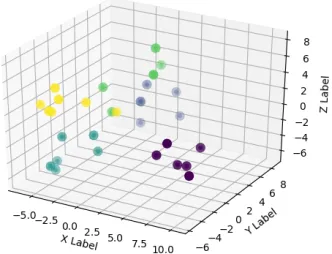
9 Two family clusters formed by DALI in 3D. . . 26
10 Two family clusters formed by T M-alignin 3D. . . 27
11 Two family clusters formed by EDAlign SSE in 3D. . . 27
12 Two family clusters formed by Combinatorial Extension in 3D. . . 28
13 Three family clusters formed by DALI in 2D. . . 28
14 Three family clusters formed by T M-alignin 2D. . . 29
15 Three family clusters formed by EDAlign SSE in 2D. . . 29
16 Three family clusters formed by Combinatorial Extension in 2D. . . 29
17 Three family clusters formed by DALI in 3D. . . 30
18 Three family clusters formed by T M-alignin 3D. . . 31
19 Three family clusters formed by EDAlign SSE in 3D. . . 31
21 Four family clusters formed by DALI in 2D. . . 32
22 Four family clusters formed by T M-alignin 2D. . . 33
23 Four family clusters formed by EDAlign SSE in 2D. . . 33
24 Four family clusters formed by Combinatorial Extension in 2D. . . 33
25 Four family clusters formed by DALI in 3D. . . 34
26 Four family clusters formed by T M-alignin 3D. . . 35
27 Four family clusters formed by EDAlign SSE in 3D. . . 35
28 Four family clusters formed by Combinatorial Extension in 3D. . . 36
29 Five family clusters formed byDALI in 2D. . . 36
30 Five family clusters formed byT M-align in 2D. . . 37
31 Five family clusters formed by EDAlign SSE in 2D. . . 37
32 Five family clusters formed by Combinatorial Extension in 2D. . . 37
33 Five family clusters formed byDALI in 3D. . . 38
34 Five family clusters formed byT M-align in 3D. . . 39
35 Five family clusters formed by EDAlign SSE in 3 D. . . 39
36 Five family clusters formed by Combinatorial Extension in 3D. . . 40
37 Six family clusters formed by DALI in 2D. . . 40
38 Six family clusters formed by T M-alignin 2D. . . 41
39 Six family clusters formed by EDAlign SSE in 2D. . . 41
40 Six family clusters formed by Combinatorial Extension in 2D. . . 41
41 Six family clusters formed by DALI in 3D. . . 42
42 Six family clusters formed by T M-alignin 3D. . . 43
44 Six family clusters formed by Combinatorial Extension in 3D. . . 44
45 A guide tree . . . 60
46 Alignment along the tree. . . 61
47 A correspondence matrix. [Notice there are no columns with gaps in all rows.] . . . . 63
48 1DM1 . . . 64
49 1MBC . . . 64
50 1MBA . . . 64
51 Alignment of 1DM1, 1MBC, and 1MBA . . . 65
52 Flowchart of Revised-MASCOT [59] . . . 66
53 Set 1 . . . 68
54 Set 2 . . . 68
55 Set 3 . . . 68
56 Set 4 . . . 68
57 Set 5 . . . 71
58 Set 6 . . . 73
59 Set 7 . . . 74
60 Set 8 . . . 75
61 Set 9 . . . 75
62 Set 10 . . . 75
63 Set 11 . . . 76
64 Set 12 . . . 78
CHAPTER 1
Introduction
1.1
Overview
In recent years, a number of different pairwise alignment algorithm has been developed. Many
focused on the areas of computational methods for aligning pairwise protein structures. Since the
structural comparison problem is known to be np-complete, many different ways were proposed with
good approximations. The newly proposed alignment algorithms try to find the better alignment
than the previous or at least as good as an alignment achieved by the ones before.
Therefore, we have come up with an approach to evaluate some of the well- known and widely
accepted pairwise alignment algorithms proposed previously. In that case, we would be able to
examine which alignment algorithm works the best. In the process, we will also be able to reveal
the most significant similarities that are possible within a protein family.
Additionally, we have presented a heuristic algorithm for aligning multiple protein structures.
We have taken into account the progressive method in aligning the multiple proteins. To measure
the similarity between the alignment, we have used the Root Mean Square Deviation (RMSD) as
1.2
Motivation
There are basically three main classes of motives behind these work:
1. Quality of Alignment - Once we have the pairwise evaluation techniques, we will be able
to find the alignment quality of all the pairwise alignment algorithms, and as a result for
a structural comparison application, or any alignment application we will be using the best
algorithm, fetching the best results. It will be a measure to find the quality of new pairwise
alignment algorithms. In short, we will be able to get the best alignment from the best
pairwise alignment algorithm.
2. Infer Functional Properties - In the process of evaluating different pairwise alignment
tech-niques, we will eventually be able to differentiate and classify different proteins with their
functional properties. For example, proteins 1YZQ and 1T91 belongs to the same family
resulting in same structures, so we can conclude that both the proteins have the high
prob-ability of performing same functions. Thus, the evaluation technique adopted will help us
infer functional properties of an entire family or a group of unknown proteins.
3. Evolutionary Relationships - Biologists found that there are about 8 to 100 millions species
of organisms living on Earth today. How amazing it is to think about the common ancestor
of humans and mouse. A lot of studies based on the three-dimensional structures of proteins
show that two proteins with insignificant sequence similarity have a common fold and therefore
performing same or identical functions. Hence, it is useful to use the three- dimensional
structures instead of the amino acid sequence similarities in finding evolution between distant
proteins. In this work, we will be able to conclude evolutionary relationships depending on
1.3
Problem Statement and Solution Outline
In this thesis, we proposed a novel approach to measure the effectiveness of a sample of four different
pairwise alignment algorithms, DALI, TM-align, EDAlignSSE and Combinatorial Extension (CE)
for detecting structural similarities among proteins and conclude their functional properties. As
a result, we can classify them according to their families. We have come up with an approach
and carried out extensive experiments. We have prepared five different datasets, each consisting of
proteins from two to six different families. For each dataset, we computed a distance matrix, where
each distance is thecRM SDdistance of a pair of protein structures. For each distance matrix, we
used Principal Component Analysis to obtain an embedding of a set of points (each representing
a protein) that realize these distances in a two-dimensional space. To compare the clustering of
the families, we used the k-means clustering algorithm to cluster the points, sans family labels.
Our conclusion is that of the four algorithms considered, T M-align proved to be successful in
translating structural proximity to spatial proximity followed byCE.
In further addition to our work, we propose a Multiple Structural Alignment method. MSA is a
fundamental tool for correlating the structural similarity of proteins with their functional similarity.
It is a heuristic algorithm for multiple sequence alignment, we have used the Progressive Multiple
Alignment approach, in our algorithm. The steps involve building a guide tree representing the
similarity between sequences; this tree will guide us through the alignment process. We will then
build an alignment for each internal node of the tree, where the alignment at any internal node will
have all the sequences previously aligned. The root mean square deviation (RMSD) as a metric
measure of alignment quality is been used, and report this measure for a large and varied number
of alignments. We will be comparing the execution times of our algorithm with the well-known
1.4
Thesis Organization
The remainder of thesis is organized as follows. Chapter 2 explains our first problem on evaluating
various widely available pairwise alignment algorithms, it gives a detailed description of the problem
and the technique used for evaluating the various Pairwise Alignment Algorithm and outputs
the best alignment algorithm among all. Chapter 3 presents our second problem on proposing
a heuristic method in aligning more than two proteins using a progressive alignment approach.
Chapter 4 contains the conclusions acquired from the two problems.
1.5
Fundamentals of Protein and Protein Structures
1.5.1 What are Proteins?
Small molecules resulting into gigantic sequential molecules are known as Proteins [11]. Made out
of hundred different amino acids found in nature, they are connected by peptide bonds to form
single or multiple polypeptide chains of polymers. In protein synthesis process, only twenty amino
acids are created by ribosomes [59]. In the process of peptide bond formation between amino
and carboxyl acid groups from adjacent amino acids, a water molecule is released and the residue
formed is the remains of amino acid [59]. The amino acid sequence is called Primary Structure of a
protein. Each Protein has a unique structure. The backbone of a protein comes into existence only
when all the liberated amino acids have bonded together to form a residue. A protein comprises
of Nitrogen (N) atom from one amino group, central α-carbon atom, and a Carbon (C) atom
from the carboxylic group repeated in a triplet, one for each residue which have very rigid peptide
bonds between them resulting into only two rotatable bonds along the protein backbone; the bond
[59].
FIGURE 1: Amino acid Structure in Protein [33]
Thus, the complete 3D structure of proteins is determined by rotational states of the
above-mentioned bonds in every residue. The angles of these two bonds are denoted by phi and psi
[11]. There two main types of proteins, namely, Globular proteins and Fibrous proteins, of which,
the former plays an active role in the expression of genes, categorizing metabolic process and
replication; and later are more passive and often serve a structural purpose. Globular proteins are
sphere-shaped, compact, nonrepetitive, between 100 to 300 residues in size and are considered to
be the workhorses of the cell. Lastly, there are membranes, which regulates and controls various
atoms and molecules traffic across the cells [59].
1.5.2 What are their functions?
There are several functions of a protein, the main are as follows:
1. Antibody - Protein helps in binding with foreign particles to help and protect the body from
strengthens one’s immune system.
2. Enzyme - Proteins involves in chemical reactions, resulting in the formation of new molecules
by reading the information which is stored in DNA.
3. Messenger - Proteins plays a very important role in transmitting signals between cells, tissues,
and muscles to coordinate biological processes. It helps in all the biological processes needed
for the body to live and sustain.
4. Structural Component - Most importantly, proteins provides structure and support to cells
which in return, helps in moving the body and performing the daily routine need in ones’ life.
5. Transport - Proteins play a vital role in transporting atoms throughout the body by binding
itself to a particle ad carrying atoms within cells from one part of the body to another.
1.5.3 How are Proteins structured?
Protein structure organization is spread across four levels, namely, primary, secondary, tertiary and
FIGURE 2: Different kinds of Protein structures [74]
The sequential arrangement of amino acid residues, also known as protein sequence is referred
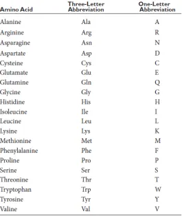
as the primary structure. The table 3 below shows the 1- or 3- letter codes that are used to denote
FIGURE 3: Amino acids in Proteins
A structure comprising of elements that are stabilized by hydrogen bonds between the carboxyl
group (C=O) and amide group (N-H) of two peptide bonds represents the secondary structure [59].
A large number of non-covalent interactions between amino acids results in three dimensional folded
arrangement of protein, which is known as the tertiary structure. When non-covalent interactions
bind multiple polypeptides into a one single larger protein, it is termed as quaternary structure.
For example, Haemoglobin, which has a quaternary structure resulting from a bond between two
1.5.4 Relatability between a pair of protein
The external conditions and chemical factors cause random genetic mutations resulting into the
metamorphosis of proteins; this is a direct consequence of relatedness between proteins. The process
of protein alignment is designed to find out the genetic information that is preserved amongst the
proteins over the time and not reversing the evolution effects [59]. Using this technique common
ancestor can be traced with the help of simulated agents which results in achieving categorization of
evolutionary similarities and differences. This further helps in building an evolutionary tree based
on which the families of different protein species can be grouped [59]. If any of the protein spices
have a common ancestor, the proteins of that species can be closely related or not relatedly at all,
depending on the evolution that might have occurred. There are 3 kinds of relatedness between
the pair of protein(s):
1. Identity: If the formations of two proteins match with each other, they are termed as identical
proteins.
2. Similarity: If the formations proteins are nearly related to each other without being identical,
they are termed as similar proteins.
3. Homology: Homology is a special case in which proteins are expected to have common
an-cestors. Creation of super families of proteins is based on two kinds of homology that protein
CHAPTER 2
Low Dimensional Clustering to Evaluate
Pairwise Protein Structure Alignment
Algorithms
2.1
Introduction
2.1.1 Life Origins
At the molecular level, protein molecules are known as the main drivers of all life processes. A
protein molecule is defined as a linear polypeptide chain, which contains adjacent pairs of amino
acids joined to each other by peptide bonds [54]. Therefore, it has the nomenclature “polypeptide”.
This linear polypeptide chain of the protein structure folds into a stable, low-energy 3-dimensional
tertiary structure to perform its respective biological function [54]. There are other different
struc-tures in protein which are formed by loops joining together two types of secondary strucstruc-tures,
known as α-helices and β-sheets.
“The most important things we know about proteins have come therefore not from theory but
observation and comparison of sequences and structures” is observed by Taylor et al. [68]. There
of this problem, as a result, it led to a board spectrum of the literature of this problem and
several large structural databases of proteins [49, 52, 30]. These databases help in classifying a
large number of protein sequences into their structurally equivalent classes using an alignment or
structure comparison algorithms.
There are namely two vital traits for pairwise protein structure alignment: (1) The way in
which folding occurs; (2) How an accurate role is performed by assuming a particular structure.
The protein folding is a well-known problem because of theorganic process drawback, predicting
how a macromolecule can fold, given the amino acid compound sequence that makes up its peptide
chain structure. A comprehensive solution is addressed for this disadvantage. The second
draw-back is that of predicting role of a known structure. Here a theoretical approach is a standard
one: structural comparison with proteins of known functions [54], which in return give rise to the
drawback of the structural alignment of a pairs of proteins.
In this work, we have come up with a solution to measure the effective of a sample of four
different pairwise alignment algorithms. The four different pairwise alignment algorithms are:
DALI, TM-Align, EDAlignSSE and Combinatorila Extension (CE).
2.1.2 Notations and Definitions of a Protein
A protein is modeled as a sequence of points,P ={pi|pi ∈R3, i= 1,2,3, ..., m}, in a 3-dimensional
Euclidean space, where m(= |P|) is the number residues and pi represents the coordinates of the
centralα-carbon atom of thei-th residue. In what follows, we will use this sequenceP to refer to
the protein it represents. [54]
Given two proteins P and Qof length mand n respectively, an alignment ofP and Q is:
[54], where 1≤i1 < i2 < ... < ik≤m and 1≤j16=j2 6=...6=jk≤n, together with
• a rigid transformation t, t(Q) = {t(qj) = q
0
j|q
0
j ∈ R3, j = 1,2,3, ..., n}, that optimizes some
similarity measure for the above correspondence [54].
2.1.3 Pairwise Protein Structure Alignment
The outline of a Pairwise Protein Structure Alignment problem is: Given two protein structures,
we find the transformation that produces the best superposition of one protein onto the other.
From the computational point of view, the rotations and the translations required by one of the
points set (protein A) which will produce a comparatively large superimpositions on the other set
(protein B). The fundamental question to this problem is: How to find the best superposition of
two protein structures? The problem of superimposing two structures of proteins is easy if we know
the equivalent amino acids in both the structures. The hard part is to find this mapping of the
corresponding atoms between two different protein structures.
Understanding a protein model clearly that will be used, is a vital step to design a pairwise
alignment algorithm. Some of the previous alignment algorithms expressed the protein model as
the centralαcarbon atom of every residue that are attached sequentially to form a polygonal chain
in three dimensions [54]. In a more primitive model, protein is viewed as a collection of points
(again theα carbon atoms) in 3-D space, where the alignment problem is allowed to view as that
of matching two point sets [54]. However, it is crucial to supplant these different kinds of models
with different features of the proteins like hydrophobicity, exposure to solvents, mutual affinities of
2.1.4 Similarity Measures
The root mean square deviation (RM SD) is widely used [37, 38] to measure the extent of structural
similarity of two proteins. There are basically two differentRM SD [79, 62, 63, 81] measures that
have been proposed in the background study:
1. coordinate root mean square deviation (cRM SD)
2. distance root mean square deviation (dRM SD)
For any two aligned structures of proteinsP andQof lengthk, these are defined as below [54].
dRM SD= v u u t
2 k2−k
k−1
X
u=1
k
X
v=u+1
(kpiu−pivk −(kqju−qjvk)2 (1)
cRM SD= v u u t 1 k k X u=1
kpiu−t(qju)k
2. (2)
[54] The similarity measures, cRM SD and dRM SD, are both concerning absolute distances,
therefore, the value ofRM SD gets poor even if there is any small presence of outliers irrespective
of the fact that the two structures are globally similar to each other theRM SDvalue will be poor.
Many other researchers [81, 37, 70, 43] have observed such similar kind of behavior. Zhang and
Skolnick [80] came up with a solution to overcome this problem, a sequence independent structural
alignment measure (TM-score) which is a variation of a metric, originally defined by Levitt and
Gerstein [41] [54]. Xu and Zhang have done a critical assessment of this TM-score. [76].
Given two proteins, a template protein P and a target protein Q, |P| ≥ |Q|, the structural similarity is obtained by a spatial superposition ofP andQthat maximizes the following score [54]
TM-score = 1
|Q|
k
X
i=1
1
1 + (di
d0)
wherekis the number of aligned residues ofP andQ;di is the distance betweeni-th pair of aligned
residues and d0(= 1.243
p
|Q| −15−1.8) is a normalization factor [54].
When the value of d0 in equation (3) is set to 5Ao, the resulting TM-score is known as a raw
TM-score (rTM-score) [54].
Xu and Zhang [76] observed that two proteins are structurally similar and belong to the same
fold when the TM-score >0.5 [54].
2.2
Prior Work
The protein structure alignment problem is a vital issue in structural bioinformatics. All the protein
alignment algorithms work mainly in three stages: finding correspondence between atoms, obtaining
a rigid transformation in space for aligning them together and finally measure the similarity between
the two aligned protein structure. The difference between all the protein structure alignment
algorithm lies on the principle or the method chosen to find the correspondence between the atoms.
Additionally, the similarity measure taken into account is different for different pairwise algorithm,
which helps in refining the correspondence for a better similarity value.
2.2.1 DALI
DALI (Protein structure comparison by alignment of distance matrices [29]) is a distance matrix
alignment method developed by Lisa Holm and Chris Sander. The DALI [29] method is based on
the fact that similar 3-dimensional structures have similar intra-molecular distances. However, the
main idea of this method revolves around the representation of each protein in a 2-dimensional
matrix storing their intramolecular distances. It tries to overlap a matrix of one protein on top of
the best match is found between the two matrices [29].
The actual implementation can be broken into three steps:
1. The method decomposes each distance matrix into contact patterns as small sub-matrices
which are of fixed sizes (hexapeptide-hexapeptide contact patterns)
2. Then it compares the contact patterns and tries to pair-up the sub-matrices, one from each
protein, which is similar and storing the matched pairs in a pair list.
3. Finally, it assembles the similar sub-matrix pairs in the correct order to obtain the overall
alignment.
2.2.2 TM-Align
TM-align: a protein structure alignment algorithm based on the TM-score [81] is a pairwise
align-ment method developed by Yang Zhang and Jeffrey Skolnick. The algorithm is nearly four times
faster than Combinatorial Extension method and 20 times faster than DALI and SAL [81].
Re-garding accuracy and coverage, the resulting structure is higher than any of the ones provided by
other most often-used methods. This method uses the TM-score rotation matrix to increase the
speed of the process by identifying the best structure alignments.
The method involves mainly of two steps:
1. Identifying initial structural alignments
2. Feed the obtained initial structural alignments into an iterative heuristic algorithm
The algorithm performs three different kinds of initial alignment :
1. The first alignment is obtained by aligning the secondary structures elements (SSEs) of two
is assigned to be 1 or 0 depending on whether or not the secondary structure elements of
aligned residues are identical. The penalty values of 1 for gap-opening works the best [81].
2. The second alignment is based on the gapless matching of two protein structures. For the
smaller of the two proteins, a gapless threading against the larger structure is performed,
then the one with the best TM-score is selected [81].
3. The third initial alignment is obtained by Dynamic Programming using a gap-opening penalty
of 1, but the score matrix used for the alignment is a half/half combination of the Secondary
Structure score matrix [81].
Finally, the algorithm feeds the initial three structural alignments to a heuristic iterative algorithm,
which is widely used in refining NP-hard structure-based alignments
2.2.3 EDAlign SSE
The EDAlign SSE (An eigendecomposition method for protein structure alignment [54]) is a
pair-wise alignment method developed by Satish Ch. Panigrahi and Asish Mukhopadhyay. This method
is designed for both equal length and unequal length proteins. In this method, protein is considered
as a polygonal chain of carbon residues in 3D. The solution of this method is depended on a matrix
eigendecomposition method to the protein structure alignment problem [54]. Finally, this
proce-dure reduces the protein structure alignment method to an approximate solution of a weighted
graph matching problem. To measure the similarity between two aligned proteins it uses TM-score
and cRMSD as the metrics [54].
For aligning equal length proteins, it refines the correspondence obtained from the matrix
correspondence. However, for the unequal length proteins, it works in three steps:
1. finds a correspondence between secondary structure elements (SSE-pairs);
2. finds a correspondence between residues within SSE-pairs;
3. applies a rigid transformation to obtain a structural alignment in space.
The final two steps are repeated until there is no further improvement found in the alignment.
2.2.4 Combinatorial Extension
Combinatorial Extension (Protein structure alignment by incremental combinatorial extension (CE)
of the optimal path [63]) is an alignment algorithm developed by I N Shindyalov and P E Bourne.
Combinatorial Extension method work with aligned fragment pairs in every step of the method.
At first, it breaks each structure in a series of fragments then tries to reassemble the fragments into
a complete alignment. An alignment fragment pair is defined as a continuous sequence of protein A
aligned against a continuous sequence of another protein B of same size [63]. Ifn1 andn2 are the
lengths of protein A and proteinB, and AFP length is set to m, then there is a total of (n1−m) X (n2−m) AFPs. These series of pairwise combination of fragments which are called aligned fragment pairs (AFPs) defines a similarity matrix. This matrix helps in generating an optimal
path to identify the final alignment. This optimal path increases linearly through the sequences,
extending the alignment [63].
The algorithm steps are as follows:
1. Select some initial Aligned Fragment Pairs (AFP)
2. An alignment path is built gradually by incrementing AFPs in a way that satisfies a certain
3. Step (2) is repeated until each protein’s length is traveled, or until no good AFPs remain
The Combinatorial Extension algorithm is a fast and accurate method that helps in finding an
optimal structure alignment. It is suitable for analysis of large protein families
2.3
Proposed Approach and Details
2.3.1 Algorithm description
Our approach can be broken up into four major steps.
1. Creating protein datasets, each consisting of proteins from up to six different families of
homologous proteins.
2. Constructing cRMSD distance matrices for each dataset, by running the selected pairwise
alignment algorithms.
3. Using Principal Component Analysis [27] to embed the points that realize the distances in
low-dimensional spaces
4. Applying a clustering algorithm to the embedded points, sans family labels, to test how
well the alignment algorithms have succeeded in translating structural proximity to spatial
proximity.
2.3.2 Creating Datasets
We have selected protein families which are completely different from one another structurally,
implying divergence in functional behavior. The proteins that make up our datasets have been
• Myosins: a class of motor proteins that are crucial to muscle contraction and other motility processes in eukaryotes.
• GTPases: a large family of hydrolase enzymes that bind and hydrolase guanosine triphosphate (GTP). These help in regulating cell growth, cell differentiation, and cell migration [1].
• Caspases : a family of protease enzymes playing essential roles in programmed cell death and inflammation [12].
• EF-Hand Proteins : a large family of calcium-binding proteins, each with an EF-hand or alpha-loop-alpha motif [42].
• Calmodulin is a calcium transducer. It is a calcium-binding protein that can bind to and regulate the functions of different protein targets, thereby affecting many different cellular
functions [46].
• Phosphotransferase: a class of enzymes that catalyze phosphorylation reactions [73]. Phos-phorylation is crucial for protein function as it activates or deactivates nearly half of the
enzymes. It is also a frequently-occurring post-translation modification in eukaryotic cells
[73].
• Cyclophilins: a family of proteins found in vertebrates and other organisms that bind to cyclosporin A, an immunosuppressant commonly used to suppress rejection after an internal
organ transplant [16].
The five datasets below were created from the above protein classes.
Family No. Family Name Proteins (PDBs)
1 GTPases 1YZQ, 1T91, 1YR9, 1XTS, 1MKY, 1PUJ, 2RCN, 2MSC, 2X2E, 1CEE
2 Myosins 1W7J, 1W7I, 1B7T, 1OE9, 2AKA, 2MYS, 4P7H, 2EC6, 2OS8, 2OGT
2. Three families, each consisting of 10 proteins
Family No. Family Name Proteins (PDBs)
1 GTPases 1YZQ, 1T91, 1YR9, 1XTS, 1MKY, 1PUJ, 2RCN, 2MSC, 2X2E, 1CEE
2 Myosins 1W7J, 1W7I, 1B7T, 1OE9, 2AKA, 2MYS, 4P7H, 2EC6, 2OS8, 2OGT
3 Caspases 1F1J, 1NW9, 1K86, 1QDU, 2C2O, 2H5I, 2NN3, 2CNK, 2CNL, 2CNN
3. Four families, each consisting of 5 proteins
Family No. Family Name Proteins (PDBs)
1 Caspases 3DEI, 2C2O, 1K86, 2H5I, 1QDU
2 Myosins 2AKA, 2EC6, 1OE9, 1B7T, 4P7H
3 ER Hand Proteins 1XO5, 1IJ5, 2BE4, 2KQ6, 5BFX
4 Calmodulin 1CLL, 1CFC, 3CLN, 1MXE, 1DMO
Family No. Family Name Proteins (PDBs)
1 Caspases 3DEI, 2C2O, 1K86, 2H5I, 1QDU, 1RHK
2 Myosins 2AKA, 2EC6, 1OE9, 1B7T, 4P7H, 1W7I
3 ER Hand Proteins 1XO5, 1IJ5, 2BE4, 2KQ6, 5BFX, 1JUO
4 Calmodulin 1CLL, 1CFC, 3CLN, 1MXE, 1DMO, 2F2P
5 Phosphotransferase 2B0G, 1FYN, 2HWG, 1J7U, 1ND4, 4ORK
5. Six families, each consisting of 7 proteins
Family No. Family Name Proteins (PDBs)
1 Caspases 3DEI, 2C2O, 1K86, 2H5I, 1QDU, 1RHK, 1V0D
2 Myosins 2AKA, 2EC6, 1OE9, 1B7T, 4P7H, 1W7I, 1BR4
3 ER Hand Proteins 1XO5, 1IJ5, 2BE4, 2KQ6, 5BFX, 1JUO, 1JFK
4 Calmodulin 1CLL, 1CFC, 3CLN, 1MXE, 1DMO, 2F2P, 2K0F
5 Phosphotransferase 2B0G, 1FYN, 2HWG, 1J7U, 1ND4, 4ORK, 1PNJ
6 Cyclophilins 1CWA, 1M9C, 1AK4, 2CPL, 2RMB, 2Z6W, 1NMK
2.3.3 Running Pairwise Alignment Algorithms on the Datasets
For each dataset, we ran the four pairwise alignment algorithms, DALI [29], T M-align [81], CE
[63] and SSEAlign [54], on each pair of proteins in the set to create a distance matrix. The
distances are the cRM SD values of all the pairs. For example, from the first dataset, consisting
2.3.4 Principal Component Analysis
Principal Component Analysis [27] is a dimensionality reduction technique that makes it possible
to visualize data in low-dimensional spaces.
In this method, a new set of variables are obtained from the existing set of variables by a linear
combination of the existing variables. The new set of variables are called Principal Components.
The components are obtained in such a manner that the first one accumulates the maximum
variation of the existing data. The succeeding component has the next highest variation and so on.
In whatever reduced dimension the existing data is embedded, this process preserves the highest
possible variance of the original set of data [57].
2.3.5 K-Means Clustering Algorithm
The k-means clustering algorithm partitions a set of n data points in a m-dimensional Euclidean
space intok-clusters. Each cluster consists of data points closest to the cluster center. The
param-eter kis part of the input to the clustering algorithm.
The data points are obtained by applying Principal Component Analysis to the cRM SD
dis-tance matrix. The returned set of points (representing proteins) lie in a low dimensional space (we
have chosen two as the embedding dimension). The visualization of these points with their family
labels shows a natural clustering that demonstrates how well an alignment algorithm translates
FIGURE 4: An example of how KMeans clustering look. [55]
When the same set of points, sans family labels, are subjected to the k-means clustering
al-gorithm which uses only the spatial proximities of the points, we expect the clustering to remain
largely unchanged with respect to the natural clustering. We discuss how well the four alignment
algorithms have fared with respect to our expectations in the section on experimental results.
2.3.6 Proposed Algorithm for Evaluating Pairwise Alignment Algorithms
We call our algorithm EP AA, short for Evaluating Pairwise Alignment Algorithms. Below, we
Algorithm 1 EP AA
1: forEach alignment algorithm, Ado 2: for Each dataset,DS do
3: Run Afor every pair of proteins to build a cRM SD distance matrix
4: Input the distance matrix to the PCA algorithm to obtain a two dimensional embedding
5: Run the k-means clustering/k-medians clustering method on the embedded point set
6: Plot the points with original family labels
7: Plot the clusters obtained from thek-means/k-medians algorithm, sans family labels
8: end for
9: end for
2.4
Experimental Results and Discussion
Experimental results obtained in 2-dimensional and 3-dimensional plots
1. Dataset 1- Two families, each consisting of 10 proteins
(a) Known Family Labels (b) k-means clusters (c) k-medians clusters
(a) Known Family Labels (b) k-means clusters (c) k-medians clusters
FIGURE 6: Two family clusters formed byT M-alignin 2D.
(a) Known Family Labels (b) k-means clusters (c) k-medians clusters
FIGURE 7: Two family clusters formed by EDAlignSSE in 2D.
(a) Known Family Labels (b) k-means clusters (c) k-medians clusters
FIGURE 8: Two family clusters formed byCombinatorialExtension in 2D.
and Fig. 8a) and the spatial clustering (Fig. 6b and Fig. 8b) are quite similar. The same
cannot be said ofDALI (Fig. 5) andSSEAlign(Fig. 7). In each of those cases, the proteins
do not form two clearly distinguishable spatial clusters. For both DALI and SSEAlign, all
the proteins except one got clustered in the same family. But, for T M-align and CE all
proteins got clustered according to their family.
We have also used kmedians clustering to verify our result in terms of family mix. Referring
to (Fig. 6c and Fig. 8c) of T M-align and CE, the spatially clustering using kmedians is
similar to the the spatially clustering obtained by kmeans clustering whereas, forDALI and
SSE (Fig. 5c and Fig. 7c), the spatial clustering are different than structural clustering.
(a) Known Family Labels (b) Clusters with unknown family labels.
(a) Known Family Labels (b) Clusters with unknown family labels.
FIGURE 10: Two family clusters formed byT M-alignin 3D.
(a) Known Family Labels (b) Clusters with unknown family labels.
(a) Known Family Labels (b) Clusters with unknown family labels.
FIGURE 12: Two family clusters formed by Combinatorial Extension in 3D.
Referring to Figs.9-12, we find that even in the higher dimensional plot, DALI (Fig. 9),
SSEAlign (Fig. 11), T M-align (Fig. 10) and CE (Fig. 12) obtains the same clustering
obtained in their 2-dimensional plot. This shows, there is no change in any family clustering
when the dimension changes from 2D to 3D. The result is same for both the dimensional plot.
2. Dataset 2- Three families, each consisting of 10 proteins
(a) Known Family Labels (b) k-means clusters (c) k-medians clusters
(a) Known Family Labels (b) k-means clusters (c) k-medians clusters
FIGURE 14: Three family clusters formed by T M-alignin 2D.
(a) Known Family Labels (b) k-means clusters (c) k-medians clusters
FIGURE 15: Three family clusters formed by EDAlign SSE in 2D.
(a) Known Family Labels (b) k-means clusters (c) k-medians clusters
FIGURE 16: Three family clusters formed by Combinatorial Extension in 2D.
structural clustering (Fig. 13a and Fig. 15a, respectively) and the spatial clustering (Fig. 13b
and Fig. 15b respectively) are very different. None of their clusterings resembles their actual
family clustering. For both of them, two families out of three got mixed up in the spatial
clustering. In the case ofT M-alignandCE, the structural clustering (Fig. 14a and Fig. 16a)
and the spatial clustering (Fig. 14b and Fig. 16b) are the same. All the three families can
be easily distinguished from the clusters formed. All the three families are well-clustered
spatially according to their structural clustering.
Referring to (Fig. 14c and Fig. 16c) of T M-alignand CE, the spatially clustering is similar
to the spatially clustering obtained by kmeans clustering. It is not the same for DALI and
SSE (Fig. 15c and Fig. 13c), the spatial clustering obtained the kmedians clustering has also
mixed all the family.
(a) Known Family Labels (b) Clusters with unknown family labels.
(a) Known Family Labels (b) Clusters with unknown family labels.
FIGURE 18: Three family clusters formed by T M-alignin 3D.
(a) Known Family Labels (b) Clusters with unknown family labels.
(a) Known Family Labels (b) Clusters with unknown family labels.
FIGURE 20: Three family clusters formed by Combinatorial Extension in 3D.
Referring to Figs.17-20, we can say that even in this dataset the higher dimensional plot of,
DALI (Fig. 17), SSEAlign (Fig. 19), T M-align (Fig. 18) and CE (Fig. 20) obtains the
similar clustering achieved in 2D with this dataset, again proving the fact that the clustering
is not affected with the dimension of plot.
3. Dataset 3- Four families, each consisting of 5 proteins
(a) Known Family Labels (b) k-means clusters (c) k-medians clusters
(a) Known Family Labels (b) k-means clusters (c) k-medians clusters
FIGURE 22: Four family clusters formed byT M-alignin 2D.
(a) Known Family Labels (b) k-means clusters (c) k-medians clusters
FIGURE 23: Four family clusters formed by EDAlign SSE in 2D.
(a) Known Family Labels (b) k-means clusters (c) k-medians clusters
FIGURE 24: Four family clusters formed by Combinatorial Extension in 2D.
the spatial clustering (Fig. 22a) of the three families are very similar followed byCE where
two families out of 4 are well clustered. But in case ofDALI (Fig. 21), the spatial clustering
of nearly all the families are dispersed. From Figs. 23a and 23b, we can say that the clustering
inSSEAlign is better than that ofDALI as it has formed proper spatial clustering in two
families out of four. However, none is as good asT M-align.
Referring to (Fig. 22c and Fig. 24c) ofT M-align and CE, the spatially clustering obtained
by k-medians has successfully clustered two-three families correctly unlike DALI and SSE
(Fig. 21c and Fig. 23c), they got wrongly clustered even using k-medians clustering.
(a) Known Family Labels (b) Clusters with unknown family labels.
(a) Known Family Labels (b) Clusters with unknown family labels.
FIGURE 26: Four family clusters formed byT M-alignin 3D.
(a) Known Family Labels (b) Clusters with unknown family labels.
(a) Known Family Labels (b) Clusters with unknown family labels.
FIGURE 28: Four family clusters formed by Combinatorial Extension in 3D.
Referring to Figs. 25-28, it again proves there is no change in any of the family clustering
when the dimensions change from 2D to 3D.DALI(Fig. 25),SSEAlign(Fig. 27),T M-align
(Fig. 26), andCE (Fig. 28), all of them, resemble the same clustering as in 2D.
4. Dataset 4- Five families, each consisting of 6 proteins
(a) Known Family Labels (b) k-means clusters (c) k-medians clusters
(a) Known Family Labels (b) k-means clusters (c) k-medians clusters
FIGURE 30: Five family clusters formed by T M-alignin 2D.
(a) Known Family Labels (b) k-means clusters (c) k-medians clusters
FIGURE 31: Five family clusters formed by EDAlign SSE in 2D.
(a) Known Family Labels (b) k-means clusters (c) k-medians clusters
FIGURE 32: Five family clusters formed by Combinatorial Extension in 2D.
(Fig. 30a and Fig. 32a) and the spatial clustering (Fig. 30b and Fig. 32b) are similar for two
to three families out of 5. Unlike DALI (Fig. 29) and SSEAlign (Fig. 31). We see that
SSEAlign has got one family clustered properly, as compared toDALI which has failed for
this large dataset. In this huge dataset, T M-align andCE behaved similarly.
Similarly for this dataset, we again find that T M-alignandCE (Fig. 30c and Fig. 32c), the
spatially clustering obtained by k-medians is same as k-means clustering. But even using
k-medians, DALI and SSE (Fig. 21c and Fig. 23c), have proved that they are unsuccessful
in translating structural proximity to spatial proximity.
(a) Known Family Labels (b) Clusters with unknown family labels.
(a) Known Family Labels (b) Clusters with unknown family labels.
FIGURE 34: Five family clusters formed by T M-alignin 3D.
(a) Known Family Labels (b) Clusters with unknown family labels.
(a) Known Family Labels (b) Clusters with unknown family labels.
FIGURE 36: Five family clusters formed by Combinatorial Extension in 3D.
Referring to Figs. 33-36, it shows even when the dataset gets higher along with the
dimen-sions, the spatial clustering is unaffected.
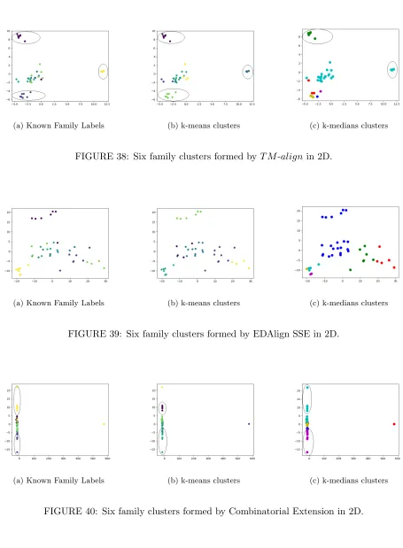
5. Dataset 5- Six families, each consisting of 7 proteins
(a) Known Family Labels (b) k-means clusters (c) k-medians clusters
(a) Known Family Labels (b) k-means clusters (c) k-medians clusters
FIGURE 38: Six family clusters formed byT M-align in 2D.
(a) Known Family Labels (b) k-means clusters (c) k-medians clusters
FIGURE 39: Six family clusters formed by EDAlign SSE in 2D.
(a) Known Family Labels (b) k-means clusters (c) k-medians clusters
FIGURE 40: Six family clusters formed by Combinatorial Extension in 2D.
thanT M-align. The structural clustering (Fig. 39a) and the spatial clustering (Fig. 39b) of
SSEAlignare similar for four families unlikeT M-alignwhich has similar clustering for three
families. Most of the families are easily distinguishable. From Fig. 37a and Fig. 37b, we find
that the structural clustering and the spatial clustering for DALI again proves to be the
worst with the proteins from different families all dispersed among the different clusters.
Finally, even in the last set using kmedians clustering, T M-align and CE (Fig. 38c and
Fig. 40c), has successfully clustered according to the family. But, DALI and SSE (Fig. 37c
and Fig. 39c), have proved mixed up the families again and proved that they are unsuccessful
in translating structural proximity to spatial proximity.
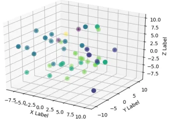
(a) Known Family Labels (b) Clusters with unknown family labels.
(a) Known Family Labels (b) Clusters with unknown family labels.
FIGURE 42: Six family clusters formed byT M-align in 3D.
(a) Known Family Labels (b) Clusters with unknown family labels.
(a) Known Family Labels (b) Clusters with unknown family labels.
FIGURE 44: Six family clusters formed by Combinatorial Extension in 3D.
Referring to Figs.41-44, it resembles the same family cluster as it gets clusters in the 2D
dimensional plot.
2.5
Conclusions
The above experiments showed that T M −Align and CE are able to cluster proteins from the same family spatially. Among all the four different algorithms taken into consideration, these
two pairwise alignment algorithm has been successfully correlated structural proximity to spatial
proximity. We have also confirmed our results by two ways:
1. Plotting in higher dimesnions to find if the cluster formation is same in both the dimension:
We applyed the same method on a little higher dimensional data (3D), even on 3D dimensional
dimension had increased.
2. Used K-median clustering, which is known to be robust in nature: This clustering also
ob-tained the similar family mix inDALIandSSEand proper clustering inT M-alignandCE,
as obtained in k-means clustering. It has showed that theT M-align and CE have
success-fully translated structural proximity to spatial proximity butDALI and SSE has again got
family mixed in the kmedians clustering
This work can be extended further by adding more pairwise alignment algorithms which are
pro-posed in the past, to test and evaluate their ability to detect structural similarity among proteins.
It can be used as a measure to find how good is the alignment algorithm. The paiwise alignment
al-gorithm is considered to be more effective, if it has successfully been able to translate the structural
CHAPTER 3
Revised-MASCOT using Progressive
Approach
3.1
Introduction
The Multiple Protein Alignment problems have received a lot of attention from Structural Biologists
because classification of protein structures and predicting their functions along with the other
newly-sequenced proteins are done by the Multiple Structure Alignment Algorithm. It is also used for
comparing the protein structures with the proteins of known functionalities. Additionally, the need
for fast, robust and reliable MStA algorithms cannot be ignored because of the increased growth
of the Protein Data Bank.
Based on the technique used, MStA algorithms can be classified roughly into one of four
cate-gories: MUSTANG [39], msTali [61], and CE-MC [22] imitates the progressive alignment approach
used for multiple sequence alignment [59]. These algorithms using the progressive approach have
succeeded in aligning multiple proteins way better than any other approaches. However, they fail in
guaranteeing convergence to the global optimum [59]. There are other algorithms which are based
on different approaches [47, 78] than progressive ones that have outperformed the progressive ones,
Mass [14], Mapsci [32], and Smolign [64], which is taken into account when the goal is to find a
struc-turally conserved subset of residues among the proteins to obtain knowledge about their evolution
and origin. It refines the consensus structure, with repetitive iterations, and finds a core common
to all the input proteins [59]. Unfortunately, such cores are pseudo-structures that, although
geo-metrically interesting, are bereft of any biological significance. There is another method designed
by Ye and Godzik which is graph-based POSA [78] which represents a protein as a directed acyclic
graph (DAG) of residues, connected sequentially following the backbone of the protein structure.
POSA creates a combined non-planar, multi-dimensional DAG, taking hinge rotation and coming
up with residue equivalences among all the input proteins. Though POSA is known to incorporate
the protein structures’ flexibility, it completely misses the motifs on TIM-barrel and helix-bundle
proteins [64], and incur a higher cost of alignments, for instance, MATT [47] or Smolign [64]. The
pivot-based approach selects one of the input molecules, closest to all the other proteins as the
pivot [59]. To obtain residue-residue correspondences, rest of proteins are aligned iteratively to the
pivot either bottom-up manner [71] or top-down manner [77]. These correspondences are required
to minimize some objective function and define a score as a similarity measure [59]. Mistral [48],[71]
and [77] are some of the few published algorithms on this approach.
Our approach to this MStA problem is using the Progressive Alignment method used for
mul-tiple sequence alignment (MSA). We propose a new algorithm, Revised MASCOT (acronym
forRevised Multiple Alignment of Structures using CenterOf proTeins), which is very similar
to the MASCOT [59] algorithm instead of using the center star method, we have taken the
pro-gressive method and tried aligning two or more protein structures together. Since we all know,
SSEs are fundamental components of protein structures which serves as well-preserved scaffolds,
important information about the secondary structural elements (SSEs) [59]. Mutations do affect
the loops which result in modifying the functionality, but the SSEs are evolutionarily remarkably
conserved. For example, the substrate specificity of different serine proteases is governed by the
confirmation of the binding loops [25]. Representing protein structures using their SSEs are also
used on several pairwise alignment problems [36], [3], [4]; [21], [44].
In this paper, our goal is to design and develop a fast, elegant algorithm that uses the sequences
of proteins using their SSEs to produce a structural alignment with high accuracy. Keeping this in
mind, we have designed a version of MASCOT [59] called Revised MASCOT as a similar hybrid
algorithm. It uses the most similar closely related proteins as a pair of sequences, and align those
using global alignment. Then, we identify the next most closely related sequence pair; it can be a
pair of sequences or a pair of alignments, and align them to each other. This concept of aligning two
sequences or two alignments or a sequence with an alignment is obtained by finding the minimum
sum of pairwise-distances between a pair of sequences.
Next, to align a pair of protein sequences, we find an optimal correspondence among the
al-pha carbon atom which is the backbone of the protein, using an inter-residue Euclidean distance
threshold and compares the centerRMSD of the structures aligned in space as a measure of their
similarity [59]. We have implemented Revised MASCOT and run experiments on the same set
of proteins done by MASCOT. Again similar to [59], we too have included a comparison of the
execution times of the Revised MASCOT with the well-known algorithm MUSTANG to show that
3.1.1 Algorithm Aspects
What is an Alignment?
An alignment explains patterns of matching between some form of sequences, structures, and
se-quences with structures of proteins. An alignment gives a clear idea of the function and evolutionary
distance of the proteins from a common ancestor.
Various methods like local geometry matching [75], comparison of distance matrices [28],
max-imal common subgraph detection [7], spectral matching [62], geometric hashing [51], contact map
overlap [6, 13] and dynamic programming [81, 67] are used to obtain an initial equivalence set during
alignment of two protein structures which is a 3-dimensional analogue of linear sequence alignment
of peptide or nucleotide sequences [54]. Moreover, methods such as Monte Carlo algorithm or
sim-ulated annealing [28], dynamic programming [81, 67, 17, 18], incremental combinatorial extension
of the optimal path [63] and genetic algorithm [66] can be used to further optimize these previously
obtained equivalence set a goal to measure the amount of structural similarity for alignment of
protein residue. This similarity measure is classified into four different categories (1) distance map
similarity [28, 69, 5, 53] (2) root mean square deviation (RMSD) [62, 81, 63, 79] (3) contact map
overlap [20] (4) universal similarity matrix [40, 56] are used to quantify the structural similarity;
but even after all these classifications and research over the years, there is no universal definition of
similarity score to measure structural similarity extent. A comprehensive list of different similarity
measures is discussed by Hasegawa and Holm [24].
Global Alignment
In Global Alignment, the sequences are aligned along their entire lengths. This method of
Alignment technique is done using the Needleman-Wunsch algorithm, which is based on dynamic
programming. The alignment received from this technique illustrates a lot about the protein and
its sequences which as a result leads to the understanding of its functions and structures.
Let Am, ... , An and Bm, ... , Bn be the two different protein sequences of length m and n
respectively which we need to align optimally. It contains input alphabets consisting of symbols
to represents different amino acids in the protein structure [59]. So, we define an alignment in a
much formal way. To perform a global alignment of A and B, we need to introduce gaps (−) at the beginning or ending or between a pair of symbols, such that the alignment which is obtained
must have the following properties.
1. It should be a 2 X L matrix where max(m,n)<= L <= m+n
2. First row has either a blank or a character from A and second row has either a blank or a
character from B.
3. No column can have blanks in both the sequences.
Needleman-Wunsch Algorithm is a global alignment method used to find the optimal edit
dis-tance between two string [50] or protein sequences. The NeedlemanWunsch algorithm performs a
global alignment on two sequences. It is an example of dynamic programming and was the first
application of dynamic programming algorithm to biological sequence comparison. It is applied to
optimization problems..
Structure Alignment
In protein structure alignment, there is a comparison taken place between the positions of atoms
determined by its 3D structure [59]. Holms and Sander stated ”Comparing protein shapes rather
than protein sequences are like using a bigger telescope that looks father into the universe, and thus
farther back in time, opening the door to detect the most remote and most fascinating evolutionary
relations” [31]. The statement means aligning the 3D structure of proteins gives more insight into
their functions and evolutionary origins [31]. For a structural alignment to take place optimally,
we must first find out which residues correspondences, it is only possible if we are unaware of the
proteins 3D structure. There is a possibility when a residue cannot be mapped to any other residue,
in that case, it will be aligned with a gap ’-’. Therefore, in a set ofN proteins, one-to-one mapping
of the protein residues gives rise to a protein structure alignment.
For two proteins of length NB and NA, the number of possible alignment grows exponentially,
min(NA,NB)
X
k=0
2k(kAN)(kNB)
The number of possible alignment increases, when the number of residues in both the proteins
is more. The problem is a pairwise alignment one, whenN = 2, for which there are many widely
accepted algorithms such as, Dali [28], SSAP [53], Eigenvalue Decomposition [54], Combinatorial
Extension [63] etc. WhenN >2, the problem is termed as Multiple Structure Alignment (MStA).
Our problem belongs to this category of problem [59].
3.1.2 Problem Statement
Consider P = P1, P2 ... PN a set of N protein structures and L1, L2 LN the number of residues
in each proteins respectively. All the protein structures are represented by the coordinates of their
alpha carbon (Cα) atoms. Pab denotes thebth residue of theath structure, for a = 1 ... N and b =
The multiple structural alignment of P is Y = (Yab) , 1 ≤a≤ N, 1≤ b≤L , such that:
• Max (L1,L2 ... LN)≤ L≤(L1 + L2 + ... + LN).
• Each element in X either has to be one of the residues of Pij or a gap which is a special null
residue, denoted by the symbol ’-’.
• Theathrow in Y contains the set of C positions of a protein structurei, it might contain gaps in between. This shows that the alignment makes sure that it preserves the order of residues.
Now that the matrix of equivalences Y are obtained, a set of rigid body transformations needs to
be done, each having a proper rotation matrixRota, where det(Rota)= +1, which can be denoted
as, TR(Rota ,T ransa ) 1 ≤i≤N, whereT ransa is a translation tuple which is acted upon each
protein in Y, which will drive an optimal superposition of all the structures.
A superposition of minimum coordinate root mean square deviation (RMSD) is obtained with
the help of an input set of reference 3D points of the equivalent residues.
RM SD= r 1 n i=1 X N
((vix−wix)
2+ (v
iy−wiy)
2+ (v
iz −wiz)
2)
where, (vix;viy;viz) represents 3D coordinates of residueiwhich are obtained by superimposing
structureaon structure b. The distances between the corresponding residuesvi and wi represents
the Euclidean distance. n denotes the number of aligned. Basically, our goal is to minimize root
mean square deviation (RMSD) while maximizing the number of aligned residues.
3.2
Prior Work
3.2.1 A center star approach - MASCOT
The center-star approach was first proposed by Gusfield [23]. This approach falls under the class
of approximation algorithms as it aims to give a solution quality and a run-time bound which can
be proved [59]. Gusfield stated the solution of Multiple Structure Alignment could be optimal up
to a constant factor 2 with the sum-of-pairs metric [23].
The following properties must be satisfied by the cost function of sequences a, b, and c:
Cost[a, a] = 0 (reflexive)
Cost[a, b] = Cost[b, a]≥ 0 (symmetric)
Cost[a, b] + Cost[b, c] ≥Cost[x, z] (triangle inequality) The center-star algorithm follows the following steps:
1. By minimizing the Sum-of-Pairs metric, we need to find the center protein sequenceSc such
that
N
X
j=1
EditDistance(Pi, Pj)
is minimum.
2. Next, align all the rest N −1 protein sequences, Si, where i = 1 ... N, and i 6= c to Sc, following once a gap always a gap policy [59].
For the first step, they perform a global alignment on every pair of protein sequences using
Needleman-Wunsch algorithm [50] which requires an affine gap opening penalty, and a scoring
![FIGURE 2: Different kinds of Protein structures [74]](https://thumb-us.123doks.com/thumbv2/123dok_us/1367921.1169541/20.612.191.419.84.416/figure-dierent-kinds-of-protein-structures.webp)
![FIGURE 4: An example of how KMeans clustering look. [55]](https://thumb-us.123doks.com/thumbv2/123dok_us/1367921.1169541/36.612.125.480.81.285/figure-example-kmeans-clustering-look.webp)