Efficient Parameter Estimation Techniques for Hysteresis
Models
J. M. Ernstberger
∗and R. C. Smith
†ABSTRACT
Actuators employing ferroelectric or ferromagnetic compounds are solid-state, efficient, and compact making them well-suited for aerospace, aeronautic, industrial and military applications. However, they also exhibit frequency, stress and thermally-dependent hysteresis and constitutive nonlinearities which must be incorpo-rated in models for accurate device characterization and control design. A critical step in the use of these models is the estimation or re-estimation of parameters in a manner that is both efficient and robust. In this presentation, we discuss techniques to estimate densities in the homogenized energy model based on Galerkin expansions using physically motivated basis functions. The yields highly tractable optimization algorithms in which initial parameter estimates can be obtained from measured properties of the data. The efficiency and accuracy of the models and estimation algorithms are validated with experimental data.
1. INTRODUCTION
Ferroelectric compounds, such as PZT (Lead Zirconate Titanate, PbTiO3), convert field energy to mechanical energy via the reorientation of specific molecules during polarization and can consequently be employed for actuation purposes. A second attribute of these materials is the conversion of mechanical to field energies enabling these materials to be used as sensors. The actuation and sensing properties of these materials may be used in tandem to create self-sensing actuators.
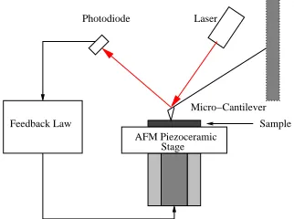
PZT is well-studied and widely employed for military and industrial use. DARPA has field-tested the equipment of infantry soldiers with boots and uniforms containing PZT plates and filaments which produce charges based upon mechanical deformations resulting in the continual recharging of field-pack batteries [1]. Industrial applications most commonly use the actuation properties of ferroelectric compounds. Figure 1 displays the schematic of the atomic force microscope (AFM) used for the imaging of structures at the atomic level where a PZT stage is used to position the sample [2]. Another application, the commercial THin layer UNimorph DrivER (THUNDER), is a thin layer of PZT over a pre-stressed brass, tin, or aluminum substrate. These devices are commonly used for pumps or flanges by arching or flattening the device via a chosen current direction [3, 4].
As transducers, ferroelectric compounds are desirable due to their light weight and solid-state construc-tion. The hysteretic and nonlinear behaviors inherent to the input-output relationship necessitate sophis-ticated control laws for usable employment in many operating regimes which may rely upon a model char-acterization of the actuator. Consequently, the estimation of key model parameters must be obtained in a manner which results in the quick and accurate quantification of such parameters.
Smart materials, such as PZT, exhibit environment-dependent behavior which, under dynamic operating conditions, can require that model parameters be re-estimated to maintain the accuracy of the model and control algorithm. Here, we present an alternate formulation of the homogenized energy model presented in [5] to reduce the computational intensity of the parameter estimation problem.
∗Department of Mathematics, LaGrange College, [email protected]
Feedback Law Photodiode
AFM Piezoceramic Stage
Laser
Sample Micro−Cantilever
Figure 1.Schematic of an atomic force microscope.
2. MODEL
We first summarize the homogenized energy model used to quantify the polarization mechanisms in the PZT-based actuator. Formulations of the local switching relation neglecting and including thermal relaxation are detailed. Finally, a detailed description of a Galerkin expansion density formulation exhibiting physical properties of the coercive and interaction field densities is given.
2.1. Homogenized Energy Model
We describe a homogenized energy model for polarization as a nonlinear function of applied electric field. This model is detailed in [5, 6] and incorporates only 180◦ switching. We begin by examining the energies inherent to the molecular structure of the ferroelectric material.
The Helmholtz energy quantifies the internal energy of dipoles and is characterized using the piecewise-quadratic relationship
ψ(P) =η 2
(P+PR)2 P ≤ −PI
(P−PR)2 P ≥PI
(PI−PR)
P2
PI −PR
|P|< PI.
(1)
Here,η is the rate of change of field with respect to polarization,PR is the remanent polarization, andPI is the positive inflection point. The Gibbs energy incorporates the workEP and is given by
G(E, P) =ψ(P)−EP (2)
and depicted in Figure 2(a). By minimization of the Gibbs energy with respect to polarization, a local polarization relation neglecting thermal relaxation can be written as
P(E+EI;Ec) =
E+EI
η +δ(E+EI;Ec)PR (3)
where
δ(E+EI;Ec) =
(
1 E+EI≥Ec −1 E+EI<−Ec.
(4)
This kernel is depicted in Figure 2(b). In (3) and (4) Ec, is the value at which dipole switching occurs from a positive to a negative orientation and is termed the coercive field value. The interaction fields,EI, are internally generated fields that are distributed about the applied field value to create an effective field,
E+EI, that acts upon the material.
A local relation for polarization can incorporate thermal relaxation via the Boltzmann relation
G(E,P)
PR
PR
PI
PI
(a) (b)
P
E
Figure 2. (a). Gibbs energy versus polarization. (b). Local negligible thermal relaxation polarization kernel as a function of the electric field.
which balances the Gibbs and relative thermal energies. As detailed in [5, 6], the likelihoods of switching are
p+−= 1 T(t)
RPI
PI−ǫe
−G(E,P)V /kTdP
R∞
PI−ǫe
−G(E,P)V /kTdP and p−+= 1 T(t)
R−PI+ǫ
−PI e
−G(E,P)V /kTdP
R−PI+ǫ
−∞ e−G(E,P)V /kTdP
. (6)
The expected positive and negative polarizations are similarly given as
hP+i=
R∞
PIP e
G(E,P)V /kTdP
R∞
PIe
G(E,P)V /kTdP and hP−i=
R−PI
−∞ P e
G(E,P)V /kTdP
R−PI
−∞ eG(E,P)V /kTdP
. (7)
We quantify the number of dipole moments as N = N−+N+ where N is the number of total dipole moments. The values N− andN+ are respectively the number of negatively and positively oriented dipole moments. The moment fractions are then
x+=
N+
N andx−=
N−
N (8)
wherex−+x+= 1. The evolution of the moment fractions are quantified by the differential equations
˙
x+=−p+−x++p−+x− and x˙− =−p−+x−+p+−x+ (9)
or the simplified form
˙
x+=−(p+−+p−+)x++p−+. (10)
The local polarization relation incorporating thermal effects is then ¯
P =x+hP+i+x−hP−i. (11)
The macroscopic polarization relation is given as
[P(E)] (t) =
Z ∞
0
Z ∞
−∞
ν1(Ec)ν2(EI)P¯(E+EI;Ec)(t)dEIdEc (12)
which incorporates material inhomogeneities via differing switching points and effective field variances as the manifestations of underlying densitiesν1(Ec) andν2(EI) defined by the properties
1.) ν1(x) is only defined for x >0;
2.) ν2(−x) =ν2(x) for density symmetry; (13)
3.) |ν1(x)| ≤c1e−a1xand |ν2(x)| ≤c2e−a2|x|.
Finally, for computational purposes, (12) may be discretized with quadrature using the relation
[P(E)] (t)≈ Ni X
i=1 Nj X
j=1
ν1 Eci
ν2
EIj hP¯E+EIj;Eic
i
2.2. Galerkin Density Representations
In [7], linear and cubic B-spline Galerkin expansion formulations of the homogenized energy model were presented. While exhibiting decreased parameter estimation runtimes in comparison to general density for-mulations [8], the resultant densities were often nonphysical and corresponding constraints were incorporated into the numerical optimization to generate expected density behaviors.
We now introduce a set of basis elements for use in a Galerkin expansion representation of the densities
ν1 andν2. Define the densities as the Galerkin expansions
ν1(Ec) = Ni X
i=1
αiφˆi Ec;µic, σci
and ν2(EI) = Nj X
j=1
βjφ˜j
EI;σjI
. (15)
We define the lognormal basis elements ˆφi as
ˆ
φi Ec;µic, σci
=√ 1
2πEcσic
e−[ln(Ec)−µic]
2
/2(σi
c)
2
(16)
where the standard deviation of each basis element is varied according to
σci =σc−vσc+
2σ
cv
Ni
i fori= 0. . . Nσ (17)
forNσ standard deviations. The mean valuesµic may also be altered in a similar fashion to that of theσic. The basis elements for the interaction field densities are defined to be be normal as
˜
φj
EI;σjI
= √ 1 2πσjIe
−E2
I/2(σ
j
I)
2
. (18)
The differing basis elements are created by adjusting the standard deviations in a manner similar to (17). These basis elements have physical interpretations and do not require constraints on the densities for decay that is required for other density representations. The only requirement imposed is the positivity of the expansion coefficients. The parameter estimation problem can now strictly be formulated as bounded optimization problem.
3. OPTIMIZATION PROBLEM
Due to the continuous formulation of the densities proposed in Section 2.2 and the known continuity of the polarization model (12),[5], a gradient-based optimization routine is chosen. We outline the method of sequential quadratic programming for this nonlinear optimization problem.
3.1. Sequential Quadratic Programming
Sequential quadratic programming (SQP) addresses the nonlinear programming problem
min
q∈Q
J(q) (19)
subject to the constraints
a(q) =0 (20)
b(q)≤0. (21)
Given the constraints (20) and (21), vectors of Lagrange multipliers u and v are introduced to form the Lagrangian
Slack variables,z, are added to the constraintsb(q)≤0 to generate the constraint
b(q) +z=0. (23)
The Lagrangian is now modified as
L(q,u,v,z) =J(q) +aT(q)u+ (b(q) +z)Tv (24)
and is subject to (20) and (23). The kthiteration of the second order Taylor series approximation for (24) is given as
L(q,u,v,z)≈L(qk,uk,vk,zk) +∇qL(qk,uk,vk,zk)Tsk+1 2 s
kT
∇qqL(q
k,uk,vk,zk)sk
where∇qL(q,u,v,z) denotes the gradient ofL(q,u,v,z) and∇qqL(q,u,v,z) is the (symmetric full-rank) Hessian ofL(q,u,v,z). The minimization problem
min
q∈Q
L(q,u,v,z) (25)
is then approximated by
min
sk
L(qk,uk,vk,zk) +∇TqL(q
k,uk,vk,zk)sk+1 2 s
kT
∇qqL(qk,uk,vk,zk)sk
(26)
and is an iterative quadratic programming problem. The constant termL(qk,uk,vk,zk) may be neglected to generate the simpler quadratic programming subproblem
min
sk 1
2 s kT
∇qqL(qk,uk,vk,zk)sk+∇qL(qk,uk,vk,zk)Tsk
. (27)
The minimum to (27) occurs atsk when
∇qqL(qk,uk,vk,zk)sk+∇qL(qk,uk,vk,zk) = 0 (28) so that
sk=−∇−qq1L(q
k,uk,vk,zk)
∇qL(qk,uk,vk,zk). (29) Equation (29) is the step in the Newton iteration with respect toq. The slack variables are updated with a corresponding stepskz. The updates for the Lagrange multipliers are also generated sequentially from the QP subproblem which can be directly derived from the first-order Taylor approximation
ai(q)≈ai(qk) + ∇qa
i(qk)T
skqfori= 1. . . NA (30)
(whereNA is the length ofa(q)). Then, if ai(q) = 0, it follows that
∇qa
i(qk)T
skq=−ai(qk). (31)
Also,
bj(q) +zj ≈bj(qk) + zkj
+ ∇qb
j(qk)T
skq+ skzj
forj= 1. . . Nb (32)
(whereNB is the length ofb(q)) which implies that
∇qb
j(qk)T
skq+ skzj
=−bj qk
+ zkj
. (33)
Then
z≈zk+skz ≥0⇒skz ≥ −zk. (34)
The parameter estimate is then updated using the iteration
qk+1=qk+αksk (35)
3.2. Gradient and Hessian Approximations
The gradient is defined as
∇qL(q,u,v,z) =
∂L ∂q1
, ∂L ∂q2
, . . . , ∂L ∂qn
T
(36)
where we approximate the partial derivatives with first-order approximates
∂L ∂qi ≈
L(q+eihkqk,u,v,z)−L(q,u,v,z)
hkqk (37)
andei is theithelementary vector. The Hessian matrix, defined as
[∇qqL(q,u,v,z)]ij =
∂2L(q,u,v,z)
∂qi∂qj
, (38)
is often implemented with the first-order approximate credited to Broyden, Fletcher, Goldfarb, and Shanno. The BFGS Hessian approximation algorithm for an objective functionalL(q,u,v,z) is:
1. H0=I,
2. Solve QP subproblem forskq,
3. Update qk+1=qk+αksk
q,
4. yk =∇qL(
qk+1,uk+1,vk+1,zk+1)− ∇qL(qk,uk,vk,zk)
αk ,
5. Using the Sherman-Morrison formula, create the low-memory version of the approximated Hessian inverse
Hk−+11 =Hk−1+
skq skqT
sTqT
yk+yTkH −1 k yk
sk
q T
yk
2 −
Hk−1yk skq T
+ skqT
yTkHk−1
sk
q T
yk
, and (39)
6. Iterate steps two through five until convergence as determined by stopping criteria with the Newton Step has occurred.
Equation (39) is a convenient formulation since αk (the line search length which can enable faster con-vergence) is adjusted at each step and the gradient of L qk,uk,vk,zk is already computed. These two alterations to Newton’s method form a Quasi-Newton iteration which converges with q-superlinear conver-gence due to the first order approximate of the Hessian matrix.
3.3. Problem Formulation
The objective functional J is posed as the squared ℓ2 residual of data versus model response and can be written as
J(q) = 1
2kP(E;q)−Pˆ(E)k 2
2 (40)
where the polarization modelPtakes a vector of electric field inputsEand the necessary model parameters
qwhich are being optimized. The parameter estimation problem is then formulated as
min
q∈Q
We have two viable kernels which may be used to model polar switching. The kernel parameters to estimate are
qk= [PR, η] (42)
for negligible relaxation and
qk = [PR, η, τ(T), γ] (43)
when thermal relaxation is included. Regardless of kernel choice, each optimization used in the results of Section 4 includes a preliminary parameter estimation where the densities are formulated as
ν1(Ec) = 1 √
2πσcEc
e−
[ln(Ec)−µc]2
2σ2c (44)
and
ν2(EI) = √ 1 2πσI
e−EI2/2σ
2
I. (45)
It then follows that
q= [qk, σ,σˆc,µˆc] (46)
where ˆµc and ˆσc are coupled to the meanµcand standard deviationσcof the underlying normal distribution ofν1(Ec) via well-known relationships.
After the preliminary estimation, the kernel parameters are retained but based upon the simpler density representation, the Galerkin expansion bases of Section 2.2 are created and the 4 +Ni+Nj parameters to be estimated are
q=
qk, α1, . . . , αNi, β1, . . . , βNj
(47)
where theαi and theβj are the coefficients of the Galerkin expansions.
4. RESULTS
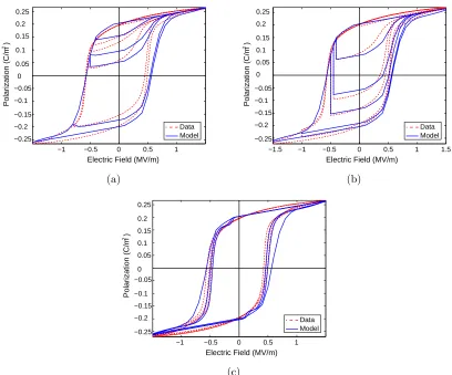
We estimate the parameters of the homogenized energy model of Section 2.1 using PZT data reported in [9]. The results displayed in Figure 3 employ seven interaction field bases in the expansion for ν2(EI) and twelve coercive field bases forν1(Ec) (four standard deviations, three means). Final parameter values were
PR = 0.20 C/m2 and η = 2.517×10⁷. For the model that neglects thermal relaxtion, fits to data are presented in Figures 3 (a) - (c) with estimated densities presented in Figure 3(d).
When incorporating thermal relaxation into the PZT characterization, we must now also estimate the parameters γ and τ(T). Final parameter estimates are PR = 2.0145×10⁻¹ C/m2, η = 2.3459×10⁷,
τ= 1.17328×101 timesteps, andγ= 8.93333×10⁻² m3/J. Fits to data are presented in Figures 4(a) - (c) with basis elements and estimated densities plottedin Figures 5 (a) - (b). The residual of the model versus data is greatly decreased and the thermal relaxation is accurately quantified for regions where the field is held constant.
5. CONCLUDING REMARKS
General density representations [8] produce highly accurate model representations but are computation-ally intense. Normal and lognormal densities can be used as representations of the interaction and coercive field densities in a low-intensity and easily estimated manner, but may not yield accurate density repre-sentations. The Galerkin expansions of Section 2.2 reduce the computational intensity of the parameter estimation problem while maintaining accurate (and physical) model characterizations.
Sequential quadratic programming was employed for the nonlinear least-square optimization with an initial of a lognormal coercive field density and a normal interaction field density. These representations created a lower-dimension parameter estimation problem which resulted in a simple and relatively accurate preliminary fit to data. A second optimization was performed using the previously discussed Galerkin expansion constructed with families of normal and lognormal basis elements. These bases are used to construct decaying densities for model characterizations that are less computationally intense and more accurate in comparison to previous quantifications.
ACKNOWLEDGEMENTS
This research was supported in part by the Air Force Office of Scientific Research through the grants AFOSR-FA9550-04-1-0203 and AFOSR FA9550-08-1-0348.
−1 −0.5 0 0.5 1 −0.25
−0.2 −0.15 −0.1 −0.05
0 0.05 0.1 0.15 0.2 0.25
Electric Field (MV/m)
Polarization (C/m )
2
Data Model
−1 −0.5 0 0.5 1 −0.25
−0.2 −0.15 −0.1 −0.05
0 0.05 0.1 0.15 0.2 0.25 0.25
Electric Field (MV/m)
Polarization (C/m )
2
Data Model
(a) (b)
−1 −0.5 0 0.5 1 −0.25
−0.2 −0.15 −0.1 −0.05
0 0.05 0.1 0.15 0.2 0.25 0.25
Electric Field (MV/m)
Polarization (C/m )
2
Data Model
0 0.5 1 1.5 0
0.2 0.4 0.6 0.8 1 1.2 1.4 1.6 1.8x 10
−5
Coercive Field (MV/m)
0 2000 4000 0
0.5 1 1.5 2 2.5x 10
−3
Interaction Field (V/m)
(c) (d)
−1 −0.5 0 0.5 1 −0.25
−0.2 −0.15 −0.1 −0.05
0 0.05 0.1 0.15 0.2 0.25
Electric Field (MV/m)
Polarization (C/m )
2
Data Model
−1.5 −1 −0.5 0 0.5 1 1.5
−0.25 −0.2 −0.15 −0.1 −0.05
0 0.05 0.1 0.15 0.2 0.25
Electric Field (MV/m)
Polarization (C/m )
2
Data Model
(a) (b)
−1 −0.5 0 0.5 1
−0.25 −0.2 −0.15 −0.1 −0.05
0 0.05 0.1 0.15 0.2 0.25
Electric Field (MV/m)
Polarization (C/m )
2
Data Model
(c)
Figure 4.Optimized thermal relaxation model fits to PZT (a) minor loop, (b) creep, and (c) major loop data from [9].
0 1 2
0 1 2 3 4x 10
−5
Coercive Field (V/m)
0 2 4 x 10
x 1060 4
0.4 0.8 1.2 1.6
x 10−4
Interaction Field (V/m)
5 10 15x 10
0 2 4 6 8
x 10−6
Coercive Field (V/m)
−4 −2 0 2 4x 10
4
2 4 6 8 10 12
x 10−5
Interaction Field (V/m)
5
(a) (b)
REFERENCES
[1] K. Mossi, Z. Ounaies, and S. Oakley, “Optimizing energy harvesting of a composite unimorph pre-stressed bender,”Sixteenth Technical Conference of the American Society for Composites, vol. 2001, 2001.
[2] R. Smith, A. Hatch, T. De, M. Salapaka, R. del Rosario, and J. Raye, “Model development for atomic force microscope stage mechanisms,” SIAM Journal on Applied Mathematics, vol. 66, no. 6, pp. 1998– 2026, 2006.
[3] K. Mossi, Z. Ounaies, R. Smith, and B. Ball, “Prestressed curved actuators: characterization and mod-eling of their piezoelectric behavior,”Smart Structures and Materials 2003: Active Materials: Behavior
and Mechanics. Edited by Lagoudas, Dimitris C. Proceedings of the SPIE,, vol. 5053, pp. 423–435, 2003.
[4] B. Ball, R. Smith, and Z. Ounaies, “A dynamic hysteresis model for THUNDER transducers,”Smart
Structures and Materials 2003: Modeling, Signal Processing, and Control. Proceedings of the SPIE,
vol. 5049, pp. 100–111, 2003.
[5] R. Smith,Smart Material Systems: Model Development. Philadelphia: Society for Industrial and Applied Mathematics, 2005.
[6] R. Smith, S. Seelecke, Z. Ounaies, and J. Smith, “A free energy model for hysteresis in ferroelectric materials,”Journal of Intelligent Material Systems and Structures, vol. 14, 2003.
[7] J. Ernstberger and R. Smith, “High-speed parameter estimation algorithms for nonlinear smart materi-als,” inProceedings of SPIE–Volume 6523: Modeling, Signal Processing, and Control for Smart Structures 2007, April 2007. 6523OS.
[8] R. Smith, A. Hatch, B. Mukherjee, and S. Liu, “A homogenized energy model for hysteresis in ferroelectric materials: general density formulation,”Journal of Intelligent Material Systems and Structures, vol. 16, no. 9, p. 713, 2005.
[9] S. Seelecke and A. York, “Experimental investigation of rate-dependent inner hysteresis loops in pzt,”

![Figure 3. Optimized negligible relaxation model fits to PZT (a) minor loop, (b) creep, and (c) major loop datafrom [9]](https://thumb-us.123doks.com/thumbv2/123dok_us/1396894.1172379/8.612.90.508.318.656/figure-optimized-negligible-relaxation-minor-creep-major-datafrom.webp)